
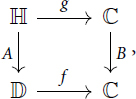
 ?Mathematical formulae have been encoded as MathML and are displayed in this HTML version using MathJax in order to improve their display. Uncheck the box to turn MathJax off. This feature requires Javascript. Click on a formula to zoom.
Abstract
It was shown by Bishop that if Thurston’s K = 2 conjecture holds for some planar domain, then Brennan’s conjecture holds for the Riemann map of that domain as well. In this paper we show numerically that the original counterexample to Thurston’s K = 2 conjecture given by Epstein, Marden and Marković is not a counterexample to Brennan’s conjecture.
1 Introduction
1.1 Thurston’s K = 2 conjecture
Let Ω be a simply connected proper subdomain of where
is the 3-dimensional hyperbolic space. Let
be the union of all hyperbolic half-spaces H such that
. Then we define the dome of Ω to be
. It is known (see the book by Epstein and Marden [Citation7] for a detailed account) that
with the path metric induced from
is isometric to the unit disk
with its hyperbolic metric. Using this isometry, we give
a conformal structure.
Note that Ω and share the common boundary
, so we set
Let be the set of all Möbius transformations that preserve Ω. Each such transformation extends to an isometry of
preserving
, so we define
Definition 1.
Given a simply connected proper subdomain Ω of the plane, we define
It was shown by Sullivan that in [Citation13]. A more detailed proof of this result and a proof that
was given by Epstein and Marden in [Citation7]. Thurston conjectured the following result.
Conjecture (Thurston’s K = 2 conjecture). For any simply connected proper subdomain , we have
.
Epstein, Marden and Marković constructed counterexamples for this conjecture in [Citation8] for the equivariant case and in [Citation10] for the general case. Komori and Matthews then constructed in [Citation12] a more explicit counterexample for the equivariant case building on the ideas of [Citation8].
1.2 Brennan’s conjecture
We remind the reader that given a simply connected proper subdomain , by the Riemann mapping theorem there exists a conformal map
. Brennan conjectured the following regarding the growth of
near
.
Conjecture (Brennan’s conjecture). Let Ω be a simply connected proper subdomain of , and let
be a conformal map. Then
for all
.
Brennan’s conjecture in full generality is still open.
1.3 Bishop’s theorem
Bishop showed in [Citation2] that if Thurston’s K = 2 conjecture holds for some domain, then Brennan’s conjecture holds for that domain as well.
Theorem 1.
Let Ω be a simply connected proper subdomain of the complex plane, and let be a conformal map. Then
for all
. In particular if
, then Brennan’s conjecture holds for Ω.
It was shown by Epstein, Marden and Marković in [Citation9] that Thurston’s K = 2 conjecture holds for domains in that are convex (in the Euclidean sense), by Theorem 1 therefore proving Brennan’s conjecture in this case. Bishop showed in [Citation3] that
for all simply connected planar domains Ω, therefore giving a new proof that
for conformal maps
.
1.4 Our results
By Theorem 1, any counterexample to Brennan’s conjecture would also be a counterexample to Thurston’s K = 2 conjecture. In this paper we investigate if Brennan’s conjecture holds for a particular counterexample to Thurston’s K = 2 conjecture.
In this section we denote the counterexample to Thurston’s K = 2 conjecture from [Citation12] by Ω. In [Citation12] it was shown that . We show numerically that Brennan’s conjecture holds for Ω.
Main result. Let be a conformal map and set
. We show numerically that
. In particular
so Brennan’s conjecture holds for Ω.
The domain Ω is a connected component of the domain of discontinuity of an explicit Kleinian once-punctured torus group. Our results strongly suggest that Brennan’s conjecture holds for all domains constructed in this way. Equivalently, our results suggest that Brennan’s conjecture holds for all quasidisks invariant under a group of Möbius transformations, such that the quotient is a once-punctured torus.
1.5 General strategy
The domain Ω has an action by a Kleinian once-punctured torus group Γ. Write for its Riemann mapping and
for its inverse. Let
be the once-punctured torus Fuchsian group obtained by conjugating Γ by F, and let
be the induced isomorphism. Let
be a fundamental domain for the action of
on
. Then
is a fundamental domain for the action of Γ on Ω.
Since Ω and Γ are known, we can numerically compute the Riemann map using Schwarz-Christoffel mappings and a polygonal approximation to Ω. The quality of this estimate deteriorates near the boundary
, making it imprecise to check if
directly. However for
, the behavior of
on
is controlled by γ and
. Therefore
if and only if a certain series over
depending on
and ρ converges.
We note that the estimates of F have higher accuracy away from . We can hence still use them to reliably estimate ρ and
. Then we use these estimates to check numerically if the series mentioned in the previous paragraph converges.
1.6 A more detailed outline of the argument and the computation
The paper is divided into a theoretical Section 2, a brief section where we describe Ω and Γ in more detail Section 3, and a numerical methods and results Section 4.
In the theory part, we show that is equal to a certain infinite series depending on
and ρ, up to a bounded multiplicative error. We do this by decomposing
into
, where
is a fundamental domain for the action of
on
. We express the integral
in terms of γ and
, up to a bounded multiplicative error. We work in greater generality, considering Riemann maps
that conjugate a Fuchsian group Γ to a Kleinian group. We do this in Section 2, where the main result is Theorem 2.
In the proof of Theorem 2, issues arise since is not assumed to be compact. This is handled by showing that on a horoball H, the derivative
achieves its minimum at the closest point of H to the origin, up to a bounded multiplicative error. This is Lemma 1 and is the most involved part of the proof of Theorem 2.
We now briefly describe how Ω is constructed in [Citation12]. They start with a hyperplane in along with a Fuchsian once-punctured torus group that preserves it. Fix a hyperbolic element in this group, and consider the orbit of its axis. This is a discrete set of geodesics, along which they bend the hyperplane. The resulting pleated plane intersects the boundary of
in a curve that bounds Ω. We give an equivalent form of their construction in Section 3 that does the bending in the complex plane, without mentioning
.
This construction makes it easy to identify a point on the boundary of Ω, and to see that the orbit of any point on is dense in
. We use this observation to construct finite polygons that approximate Ω. These approximations are described in Section 4.1.
We use Schwarz-Christoffel mappings to numerically compute an approximation to the Riemann map . This approximation is used to (numerically) compute the generators of
. This is explained in Section 4.2.
We use estimates of and ρ to compute initial terms of the sum from Theorem 2. The terms appear to decay exponentially for p < 5.52 and to increase exponentially for p > 5.54. From this we conclude the Main result. This is done in Section 4.4.
2 Theoretical results
Throughout this section, we let Γ be a Fuchsian group such that is a finite area hyperbolic surface. Let
be a conformal map, normalized so that
and
. Suppose that f conjugates Γ to a Kleinian group, and let
be the induced homomorphism. Our main theoretical result is the following estimate.
Theorem 2.
Given q > 0, there exists a constant that depends only on Γ and q such that
We now outline the proof of Theorem 2. The idea is to estimate the integral separately over and
, where
is the union of a certain Γ-invariant collection of horoballs based at fixed points of the parabolics in Γ. The proof consists of three steps.
For any horoball H in
, we let z0 be the closest point of H to the origin. We show the inequality
We show
We show the necessary bounds on g as Proposition 1 in Section 2.1. Then we derive
In Corollary 1, Section 2.2, using
In Section 2.3 we define
By equivariance of f, the derivative
Notation and conventions
We write if there exists a constant
that depends only on the variables in the subscript, so that
. We analogously write
if
and
if
and
.
We will use hyperbolic geometry in several places in this paper. We always use the metric of constant curvature –1. In particular on the unit disk we have the metric
, and on the upper half-plane
we have the metric
. Whenever we write
, we are referring to the distance coming from the hyperbolic metric on either
or
.
2.1 Univalent maps and parabolic isometries
The main result of this subsection is concerned with the growth of univalent maps g defined on the upper half-plane that commute with the parabolic γ given by
. By taking quotients
and
, g descends to a univalent map
. The estimates we show on g come from the inequalities on h and its derivatives near 0, and follow from the general theory of univalent maps.
In Section 2.1.1 we recall some general results from the theory of univalent maps. The main result there is Claim 1. Then in Section 2.1.2 we state and prove the main result of this subsection.
2.1.1 General results on univalent maps
We recall some general theorems about univalent maps, that we later use in Section 2.1.2. We then show an estimate on how closely a univalent map h follows its linear approximation near 0. This is Claim 1.
Theorem (Koebe quarter theorem). Let be a univalent function with
and
. Then
contains the disk of radius
around 0.
Theorem (Koebe distortion theorem). Let be a univalent function with
and
. Then
Moreover, the second inequality implies that for any univalent function , we have for
,
The following Claim is the estimate we use to derive Proposition 1, the main result of this subsection.
Claim 1. Let be a univalent map. Then whenever
, we have
Remark 1.
The optimal constant in Claim 1 can easily be computed from de Branges’ theorem [4]. However since this is a fairly simple result, we choose to include a more elementary proof (with a non-optimal constant) below.
Proof
of Claim 1. Without loss of generality we can suppose and
. Write
Let γ be the circle of radius centered at the origin. Then
By the Koebe distortion theorem, we have
Therefore . Therefore for
, we have
□
2.1.2 Growth of univalent maps that commute with a parabolic Möbius transformation
We now state and prove the main result of this subsection, Proposition 1. As explained at the start of this subsection, starting with a map that commutes with
, we construct a map
. We show that it extends to 0 with
and then apply Claim 1 to h. This shows how h behaves near 0, and hence how g behaves near infinity. We also obtain some information on g from the Koebe distortion theorem and the Koebe quarter theorem applied to h.
Proposition 1.
There exists a universal constant C > 0 such that the following holds. Let be a univalent holomorphic map with
. Then there exists a complex number
(depending on g) so that the following holds.
Whenever
Whenever
When
Proof.
Note that is 1-periodic, so there exists a holomorphic map
defined by
. Since g is univalent, so is h. We first show that h extends to 0.
Claim 2. The map h has a removable singularity at 0 and can be extended holomorphically so that .
Proof.
Since h is univalent, it does not have an essential singularity at 0. We extend h to 0 so that it is a meromorphic function. Let for
, and R > 0 large. Then
, and hence
This shows that h has a simple zero at 0. Hence . □
We can now apply Claim 1 to getwhenever
. We now set
, so that when
, we have
, and hence
Thereforewhere
is such that
. For C large enough, whenever
, we will have
for some integer
. We replace α with
, so that
. Since
is bilipschitz on the disk centered at 0 of radius
, we see that
and (1) follows.
To show (2), we note that for ,
By the Koebe distortion theorem, since h is univalent on the unit disk, we haveso for any C > 0 fixed,
, and we have
.
We now turn to (3). Note that . By the Koebe quarter theorem, the set
contains the disk D centered at 0 with radius
. Note that
if and only if
, so the final claim of the Proposition follows. □
2.2 Derivative bounds on a horoball
Here we give a lower bound on the derivative of a univalent map
on a horoball, assuming that f conjugates a parabolic isometry of
that preserves that horoball to a parabolic Möbius transformation. The main result is Lemma 1. This lemma is used to bound the integral
over a horoball in Corollary 1. This corollary is the result we use in the coming sections.
We first define the horoballs we will consider. All horoballs will be open. Given a horoball H, the horocycle admits a natural orientation as follows. The vector v along
at
is positive if (v, w) is a positively-oriented basis of
, where w is the vector at z tangent to the geodesic ray from z to the point at infinity of H.
Definition 2.
A horoball is
-adapted to a parabolic isometry
if the following conditions hold,
the parabolic γ preserves H,
the distance
the parabolic γ moves points on
When , we define the anchor of H to be the point
closest to the origin in the hyperbolic metric.
Definition 3.
We say that a parabolic is positive if γ moves points on
in the positive direction, for some horoball H that is preserved by γ. We say that γ is negative if it is not positive.
We note that is a positive parabolic if and only if
is a negative parabolic. It is clear from the definitions that only positive parabolics in
can be adapted to horoballs.
Remark 2.
When in the upper half-plane model, the horoballs
are
-adapted. The function
is decreasing, converges to infinity as
and to 0 as
, so by continuity
-adapted horoballs exist and are unique for all
. Any positive parabolic is conjugate to γ, so the analogous picture holds for an arbitrary positive parabolic.
Our main result is the following.
Lemma 1.
There exist universal constants such that the following holds. Let
be a univalent map, and let H be a horoball not containing 0 that is
-adapted to a parabolic
, with
. Let the anchor of H be z0. We assume that f conjugates γ to a parabolic Möbius transformation. Then for all
,
Remark 3.
It is crucial that does not contain infinity in Lemma 1. Without this assumption, the Lemma does not hold. Note that we allow f to be unbounded, or equivalently
.
Corollary 1.
Let be as in Lemma 1. Let H be a horoball not containing 0 that is
-adapted to a parabolic
, with anchor
. Then for any q > 0,
Proof.
It is standard that f conjugates γ to another parabolic . From Lemma 1 we see that
□
Proof of Lemma 1.
The desired inequality will follow from the estimates in Proposition 1. We first need to conjugate f to a map that commutes with
.
Suppose without loss of generality that γ fixes 1. We will construct a commuting square
We let for
chosen such that
. We choose B depending on finiteness of the fixed point of
.
We first give some preliminary observations that will be useful in both cases. The following Claim relates and
.
Claim 3. We have for all z,
Proof.
We have , and
. Therefore
We have , and the result follows. □
For , we write
. In particular
.
Claim 4. We have and
for all
.
Proof.
We have and
. Since the geodesic ray
contains z0, the geodesic ray
contains
. In particular
and
.
Since H is a horoball containing 1, the horoball contains infinity. Since
, the second claim follows. □
Case 1 We first assume that fixes infinity. We let B(z) = az for
chosen so that
. Since A and B are invertible, the commuting square exists by setting
. Then
conjugates
to
, and hence
conjugates
to itself. In particular
.
It follows from Claim 3 that
By Claim 4, we havewhere we used Proposition 1 in the second estimate.
Case 2Assume now that fixes a point
. Set
, where
is chosen so that
. As in Case 1, both A and B are invertible so the commuting square exists, and
.
By Claim 3,
We have
By Proposition 1, and there exists
such that
Since infinity is not in the image of f, 0 is not in the image of g. In particular by Proposition 1, . For
small enough, which corresponds to
large enough, we have
, and hence
. Therefore
Let L be small enough so that for all , we have
. Hence
Similarly we havewhere we used
in the second estimate and
in the third estimate. Therefore
, as desired.□
2.3 Dividing the disk into adapted horoballs and a cocompact subset
Recall that to show Theorem 2, we split the domain into horoballs on which we use Lemma 1, and into the orbit of a compact set. We describe this splitting here, and how to estimate the integral from Theorem 2 over translates of a compact set in the next subsection.
Let L > 0 be the constant from Lemma 1. Choose arbitrarily with
. Let
be the union over all positive parabolic
of the (open) horoball
that is
-adapted to γ. We let
be the closed Dirichlet fundamental region for Γ centered at 0, and write
.
Proposition 2.
The set is compact with 0 in its interior and is a fundamental domain for the action of Γ on
.
Proof.
Implicit in the statement of the proposition is the claim that is Γ-invariant. This follows from uniqueness of
-adapted horoballs that was explained in Remark 2. The final claim follows from this and the fact that
is a fundamental domain for the action of Γ on
.
Since has finite area, by Siegel’s theorem the Dirichlet fundamental domain is a convex hyperbolic polygon [11, Theorem 4.1.1]. It is well known that any vertex at infinity
of this polygon is a fixed point of a parabolic
[1, Theorem 9.4.5 (4)]. By replacing γv
with
if necessary, we may assume that γv
is positive. Therefore
contains horoballs
that are
-adapted to γv
, and hence based at v, for each
. Therefore
is bounded, and thus compact.
For any positive parabolic , since
, we have
. Moreover since
, we have
Therefore 0 lies in the interior of . □
2.4 Integral estimates on the lift of a compact part
Recall that one of the steps in the proof of Theorem 2 is bounding . We do this by splitting
Our goal in this subsection is to show how depends on
. This follows from the Koebe distortion theorem that guarantees that
changes at most by a constant factor over
.
Proposition 3.
For any q > 0 there exists a constant such that
for all
.
Proof.
By Proposition 2, is a compact set whose interior contains 0, so we can pick radii
that depend only on Γ such that
. Here we denote by B(z, C) the hyperbolic disk centered at z of radius C.
By the Koebe distortion theorem, we have for ,
In particular, we have .
Since , and the Euclidean diameter of the hyperbolic disk
is
up to a bounded multiplicative error, on
, we have
. In particular,
for
.
Therefore
The region contains a hyperbolic disk of radius r, and hence a Euclidean disk of radius
. Therefore
and hence
. Hence
□
2.5 Proof of Theorem 2
We note that . Differentiating at 0, we see that
. Therefore
(1)
(1)
Since γ is a Möbius transformation of the disk, we can write it as , where
and
. Therefore
(2)
(2)
Using (1), (2) and Proposition 3, we find that(3)
(3)
For any positive parabolic , by Proposition 2 we have
. Fix such a
, and let z0 be the anchor of
. Then
for some
. Hence by Corollary 1 we have
Since has hyperbolic diameter bounded over
, we have by the Koebe distortion theorem
We also have as in the proof of Proposition 3,
Therefore
Since any fundamental region intersects at most a bounded number of horoballs in
, we see that
(4)
(4)
Combining (3) and (4), we see that
3 Grafting a once-punctured torus
In this section and in the rest of the paper, denote by Ω the domain from [Citation12], and by Γ the Kleinian once-punctured torus group that acts on Ω. Here we give a construction of Ω and Γ.
In [Citation12], Ω is obtained by starting with a hyperplane in and bending it along a certain discrete set of geodesics. The result of this is a set in
that disconnects
, and Ω is one of the resulting connected components. Since here we do not work with hyperbolic space
, we give a concrete description of Ω as the union of regions in the complex plane bounded by 4 or 2 circular arcs.
In this section we work in the upper half-plane, closely following [12, §2]. We denote the Möbius transformations and subsets of with a bar to distinguish them from their counterparts in the disk model.
We start with a once-punctured torus group generated by Möbius transformations
When λ and τ are real, the group acts on
and
is a once-punctured torus. We fix
throughout, and we let
with θ a real parameter, to be set later. We denote by
the Möbius transformation obtained by setting
in the formula above, and set
. We write
. Define a natural homomorphism
by
.
Let be the ideal quadrilateral with vertices
, so that
is a fundamental domain for the action of
on
. Let Σ be the union of axes of all elements of
. Then
is a disjoint union of
, where
denotes the topological interior.
Define a map by
where
is the unique element with the property that
.
For any hyperbolic element , the axis of γ is a boundary of exactly two (ideal) quadrilaterals
of the form
for
. Order
so that
. Then
and
. Since
we can extend
over all axes in Σ that separate
and
. Denote the union of all other axes in Σ by ΣB
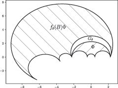
. For
there is a region
between
and
bounded by two circular arcs (see ).
Fig. 1 The gap between
and
in the image of
.
Then is simply connected and
-invariant.
Fix to be a Möbius transformation that maps
to
. Set
.
Definition 4.
We define , and
.
We also set and
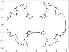
. A picture of Ω can be found in .
Fig. 2 Domain Ω.
4 Numerical results
Let be the Riemann map and
be its inverse. We denote by
and by
the homomorphism induced by f.
By a simple change of coordinates we see that(5)
(5)
By Theorem 2 and (5), for p > 2 we have if and only if
(6)
(6)
In this section we describe how we estimate ρ and , and how we estimate the range of values of p where the series (6) converges.
Since Γ is a free group of rank 2 generated by A and B (see Section 3), it suffices to estimate and
for generators A and B of Γ. As explained in Section 3, the Möbius transformations A and B are given explicitly. To estimate
and
, we estimate the Riemann mapping
using Driscoll’s Schwarz-Christoffel toolbox [Citation5, Citation6], and then compute
and
.
In Section 4.1 we describe how we get a polygon that is an approximation to Ω. Then in Section 4.2 we explain how we get estimates of
and
using this polygon and the Schwarz-Christoffel toolbox. Finally in Section 4.4 we describe how we show numerically that the sum
converges for p = 4, and we check for which values of p it diverges.
4.1 Finite polygonal approximations
We first remind the reader of some notation from Section 3. Recall that we have a once-punctured torus group of Möbius transformations acting on
, a map
, and a group isomorphism
, so that ψ is f-equivariant. Recall that
is the Möbius transformation we use to move from the upper half-plane model to the disk model.
Since is a once-punctured torus, the limit set
of
is
. Let
be the η-image of an ideal vertex of the fundamental domain
for the action of
on
. It is easy to see that
is dense in
. From the construction of ψ, we see that it extends continuously to a surjection
. Therefore
is dense in
and by equivariance
.
To obtain an approximation to , we generate some number of random points
of the form
where γ is a word in A and B of length at most some parameter
. These points determine the boundary of a polygon
which is an approximation to Ω.
Our goal to use the Schwarz-Christoffel toolbox to compute the Riemann map of this polygon. For this we need the vertices vi
to be sorted, which will almost never happen. To sort them, we note that it suffices to sort . If
, then
by equivariance.This formula is used to compute
.
The content of this subsection is summarized in Procedure Citation1. In this procedure, we use the following additional piece of notation. For a word in the free group
of rank 2, and elements
in some group G, denote by w(a, b) the element of G obtained by substituting x for a and y for b in w.
Procedure 1: Constructing finite polygonal approximations.
Input: The number of vertices n, and the maximum word length .
Output: The vertices of a polygon.
1 Construct a list of all words of length at most
in the free group
of rank
2. Pick integers uniformly at random.
3 Set and
.
4 Reorder so that
.
5 Let .
4.2 Procedure for estimating conjugated generators
Here we describe the method we use to estimate and
, assuming that we have an estimate of
. We assume that we can compute f(z) and
for any
, which is the case for Riemann mappings computed using the Schwarz-Christoffel toolbox.
More generally, we describe how to estimate for any Möbius transformation X preserving Ω. Since X preserves Ω, its conjugate
preserves the disk. It therefore takes the form
Our methods estimate and
. They are summarized in Procedure Citation2. Note that we can compute f and
at specific points. We generate some number n of points
and then compute
. We estimate
so that
is as close as possible to wi
. Specifically, we use the sum-of-squares error
In our implementation, we use MATLAB’s lsqcurvefit to do the optimization.
Procedure 2: Estimating given the Riemann mapping
and a Möbius transformation X preserving Ω.
Input: The Riemann mapping , a Möbius transformation X preserving Ω, and the sample size n.
Output: Estimate of the Möbius transformation
.
1 Generate n points uniformly at random.
2 Compute .
3 Look for the minimizers of
over
.
4 Set .
4.3 Estimates of the conjugated generators
To actually estimate generators of , we combine the procedures described in Section 4.1 and Section 4.2.
We first compute polygonal approximations to Ω using Procedure Citation1. We set the maximum word length . We construct the following approximations:
the main polygon,
several smaller polygons,
We will use to obtain estimates of
and
, and the smaller polygons
to validate these estimates.
Using the Schwarz-Christoffel toolbox, we compute the Riemann mappings and
. We use Procedure Citation2 with f, and X = A and X = B. We denote the resulting estimates
and
, and call them the main estimates in this subsection. These give the estimates of
and
that we will use in the rest of the paper.
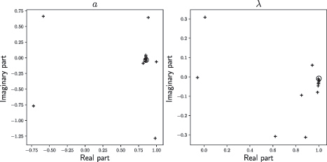
For validation, we also run Procedure Citation2 with for
, and X = A and X = B. We call the resulting estimates
and
. We plot these and the main estimates in and . We see that for each parameter, there is a clear cluster in the estimates obtained from
centered approximately at the estimate obtained from
. This suggests that
and
are accurate.
Fig. 3 The crosses represent values of parameters of a disk automorphism estimated using smaller 100-point polygonal approximations
to Ω. The circles are the estimates of λA
and aA
obtained from
.
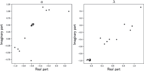
Fig. 4 The crosses represent values of parameters of a disk automorphism estimated using smaller 100-point polygonal approximations
to Ω. The circles are the estimates of λB
and aB
obtained from
.
Definition 5.
We set , where
and
We also define the homomorphism by setting
and
.
4.4 Values of p for which
By Theorem 2 and (5), if and only if
We are hence interested in values of p for which
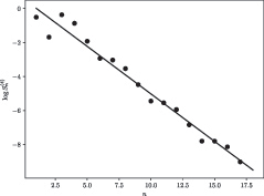
We define to be the set of all elements that have word length n in the generators
of
. We then split the above sum into
We numerically confirm that decays exponentially with n, see .
Fig. 5 The plot of as a function of n for
. The solid line is the least-squares best linear fit to the shown data points.
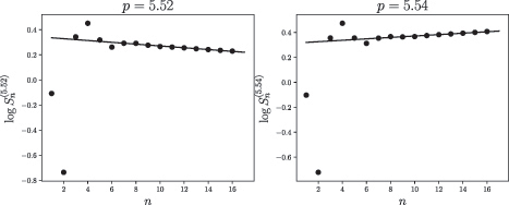
Recall the definition of from the Main result in Section 1.4,
. By Theorem 2 and (5), this is equal to
How close is to 4 gives an indication of how close the domain Ω is to being a counterexample to Brennan’s conjecture. Numerical results show that
decays exponentially with n and that
grows exponentially with n, see , meaning that
, showing the Main result.
Fig. 6 The plots of as a function of n for
and
. The solid lines are the least-squares best linear fits to the data points
for
, for
.
Acknowledgments
I would like to thank Vladimir Marković for introducing me to this problem and for his advice while working on it, and in particular for his help on Lemma 1. I would also like to thank the reviewers for pointing out an error in an earlier draft of this paper, and for their helpful comments and suggestions.
References
- Beardon, A. F. (1983). The Geometry of Discrete Groups. Grad. Texts in Math. 91. New York, NY: Springer.
- Bishop, C. J. (2002). Quasiconformal Lipschitz maps, Sullivan’s convex hull theorem, and Brennan’s conjecture. Ark. Mat. 40(1): 1–26.
- Bishop, C. J. (2007). An explicit constant for Sullivan’s convex hull theorem. In the tradition of Ahlfors and Bers III, Contemp. Math., 355. Providence, RI: American Mathematical Society, 41–69.
- De Branges, L. (1985). A proof of the Bieberbach conjecture. Acta Math. 154: 137–152. 10.1007/BF02392821
- Driscoll, T. A. (1996). Algorithm 756: A MATLAB toolbox for Schwarz–Christoffel mapping. ACM Trans. Math. Softw. 22(2): 168–186.
- Driscoll, T. A. (2005). Algorithm 843: Improvements to the Schwarz-Christoffel toolbox for MATLAB. ACM Trans. Math. Softw. 31(2): 239–251.
- Epstein, D. B. A., Marden, A. (1987). Convex hulls in hyperbolic space, a theorem of Sullivan, and measured pleated surfaces. Analytical and Geometric Aspects of Hyperbolic Space, London Math. Soc. Lecture Note Ser., 111. Cambridge, UK: Cambridge University Press, 113–253.
- Epstein, D. B. A., Marden, A., Marković, V. (2004). Quasiconformal homeomorphisms and the convex hull boundary. Ann. Math. 159(1): 305–336.
- Epstein, D. B. A., Marden, A., Marković, V. (2006). Convex Regions in the Plane and their Domes. Proc. London Math. Soc. 92: 624–654. 10.1017/S002461150501573X
- Epstein, D. B. A., Marković, V. (2005). The logarithmic spiral: a counterexample to the K = 2 conjecture. Ann. Math. 161(2): 925–957.
- Katok, S. (1992). Fuchsian groups. Chicago Lectures in Mathematics. Chicago: UCP.
- Komori, Y., Matthews, C. A. (2006). An explicit counterexample to the equivariant K = 2 conjecture. Conform. Geom. Dyn. 10(10): 184–196.
- Sullivan, D. (1981). Travaux de Thurston sur les groupes quasi-fuchsiens et les variétés hyperboliques de dimension 3 fibrées sur S1. Lect. Notes Math. 842. Berlin-New York: Springer, 196–214.