Case depth evaluation of induction-hardened camshaft by using magnetic Barkhausen noise (MBN) method

ABSTRACT

Magnetic Barkhausen noise (MBN) method is one of the non-destructive evaluating (NDE) techniques used in industry to monitor the quality of ferromagnetic products during manufacture. In this article, case depth evaluation of the camshaft lobes by this means after induction hardening is described. A routine industrial monitoring practice is found to have limitation to evaluate the thickness of this process-hardened layer. With the aid of metallography on selected samples, this uppermost layer is found to have one, or more than one microconstituents. This infers that each type possesses different physical properties in response to the MBN measurement. Consequently, the interpretation of the MBN signal/data for case depth evaluation is not straight-forward. From metallography, a qualified component should have a uniform layer of martensite with grains ≤ 50 µm and the thickness around 3.0–5.0 mm. This gives the magnetoelastic parameter (i.e. mp) in a range of 20–70 in industrial MBN measurement. The mp outside this range corresponds to either a non-martensitic type or a martensitic type with grains > 50 µm. In fact, the characteristic features of a Barkhausen burst like peak intensity, width and position can be used to categorise different microstructural conditions. Then, the case depth of the qualified components, or the thickness of the qualified martensite, can be estimated. Statistical regression decision tree model helps to divide this qualified group into three sub-groups between 3.0 and 6.0 mm, and each can be identified by the decision criteria based on the specific ranges of the mp reading, the RMS of peak intensity and the peak position. In the end, a physical model is used to show how the difference of microstructures is influencing the magnetic flux, and thus the mp. Nevertheless, more information is needed to improve the model for this application.

KEYWORDS:

• Magnetic Barkhausen noise
• induction-hardened carbon steel
• metallography
• multivariable analysis
• physical modelling

1. Introduction

Quality control (QC) by means of non-destructive evaluation (NDE) is a common means in manufacturing industry. Magnetic Barkhausen noise (MBN) method is the one suited for ferromagnetic materials. It is used in quality monitoring, case depth evaluation and grinding burn detection [1–11]. In view of case depth evaluation, via induction hardening in particular [2–11], the earliest study was found in the late 1980s by Bach [2]. When the case depth is thinner than 1.0 mm, MBN measurement generates a profile that consists of two peaks which refers to the hardened case and the softer inner core. The use of intensity ratio of two peaks is found to have a linear relationship with the case depth [2–5]. Meanwhile, the peak from the core becomes very weak when the case depth is thicker than 1.0 mm [2,5–8]. Thereby, this approach has shown its limitation. Around the mid-2000s, magnetic properties in the hysteresis loop like hysteresis loss, coercivity (H_c) and relative magnetic permeability (µ_r) are studied in parallel with the MBN profile by Lo et al. [7]. They have found certain agreements of the two results when correlate them to the case depth or the hardness depth profile. More groups have confirmed the validity of this approach [7–9]. Uniquely performed by Santa-aho, running magnetising voltage sweep (MVS) measurements under 2 magnetising frequencies show that the ratio of the two MVS slopes is giving a linear relationship with the case depth [10]. Kahrobaee takes a statistical approach by making use of the experimental data from magnetic hysteresis loop and eddy current measurements on induction-hardened components. They develop a model through principal component regression (PCR) that can distinguish the hardened sections from the non-hardened one, and is able to explain the case depth with the accuracy above 99% [11]. Still, most of these discussions are among academy, participation from industry is relatively limited. One of the ideas in this article is to bring in an industrial case study, interpret the results with the knowledge from two sides, and expand the understanding with simplified models, so the outcome is beneficial to both parties.

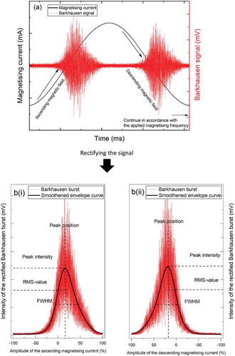
The principle of MBN is based on the study about the magnetoelastic response of a tested material. This response generates upon an alternating magnetic field stimulation from the magnetising pole pieces in a Barkhausen probe. The microscopic notion about the movement of magnetic domain wall in ferromagnetic materials refers to the change in magnetisation. This movement triggers the generation of an electrical pulse. Provided that this event happens at the uppermost surface of the tested object, i.e. between 0.01 and 1.50 mm deep [12–14], this pulse can be collected by a pick-up coil that embeds inside the sensing pole piece in the same Barkhausen probe [12–14]. The intensity and density of these discrete pulses depend on the ease of domain wall movement, domain size and domain density. Compilation of these pulses along the magnetising magnitude form a noise-like signal, which refers to a Barkhausen noise profile (Figure 1(a)). The noise level of such signal is usually expressed with a dimensionless relative scalar unit called magnetoelastic parameter, i.e. mp, which is proportional to the root mean square (RMS) of the maximum signal level after amplification and filtering, but have no direct physical meaning [15–17]. To analyse the Barkhausen noise profile, a series of noise signals developed during both ascending and descending magnetic field excitations are rectified [18] into Barkhausen bursts, as shown in Figure 1(b) [12,13,19]. Then, the fluctuation along the burst is smoothened by a numerical function into an envelope curve. The peak of the burst is then defined as the maximum value of this smoothened envelope curve, and the corresponding peak position is defined as the maximum point of a parabola curve that fits into the top 15% of the smoothened envelope. The FWHM is defined as the full width at half maximum of the smoothened envelope curve of the rectified BN burst. The RMS refers to the root mean square of the signal amplitude [12]. In fact, a precise interpretation of these results is difficult. The Barkhausen burst is an integral of characteristics from both the tested sample and the MBN apparatus. Examples of these include microconstituents, residual stress, grain size and inclusions, as well as probe geometry, probe dimension, number of turns in the magnetising coils, number of turns in the pick-up coils, the applied magnetising voltage, the applied magnetising frequency and the signal filter, etc. [1,20–22]. A more comprehensive understanding about both the sample of interest and the testing condition is needed to aid the data analysis.

Figure 1. An illustration shows (a) an alternating sinusoidal magnetic field (black) and the corresponding Barkhausen signal (red), and (b) the rectified Barkhausen bursts during (i) ascending magnetic field excitation and (ii) descending magnetic field excitation

This article focuses on an industrial case in which the MBN method is used to monitor the quality of the camshaft lobes (cam lobes) after induction hardening. In terms of quality, both the microstructure being formed and the thickness of the process-hardened layer (i.e. case depth) are of interest. While this method helps to distinguish the qualified cam lobe from the defective ones, it is difficult to determine the case depth. The current QC routine is based on mp monitoring. The measured data of lobes from 17 shafts in production are plotted in Figure 2. It shows that mp cannot directly correlate to the case depth. For the small case depth thinner than 4.5 mm, mp seems to be within a range between 20 and 70. The scattering of mp gradually increases beyond 4.5 mm. When mp is beyond 100, it can refer to a case depth of either 0.0 mm or > 5.0 mm. To look into this ambiguity, a sample piece from a qualified induction-hardened lobe is collected for cross-sectioned metallography. Based on that observation, a set of reference samples that corresponds to the individual structured layer across the surface case depth to the inner core are prepared in a separate heat-treatment experiment. The physical properties like relative magnetic permeability (µ_r) and conductivity (ơ) of individual layer are simulated through JMatPro® as described in [23]. MBN measurements are conducted for each of these references. The findings of this study help to explore the magnetic properties of microstructure in each layer and to understand the corresponding MBN parameters. This will also help to categorise the qualified induction-hardened condition and filter out the unqualified ones. After filtering, multivariable analysis is conducted on the qualified group to derive a regression decision tree model [24] that can be used for surface classification based on the experimentally produced dataset from one of the shafts. On the other hand, a numerical model based on the physical properties of materials [25] is used to simulate the depth of magnetising flux during MBN measurement.

Figure 2. Data from process monitoring of induction-hardened case depth of the cam lobes by means of MBN method

2. Case background and experimental details

Components of interest are camshafts with the composition listed in Table 1. Cam lobes on the shaft for different valve lifters were treated differently. During induction hardening, in general, the lobes were introduced into an induction coil, heated to 900–950°C for few seconds, and cooled down with fluid quenchant for a couple of cycles. The hardened region around the circumference of the lobes along the rotating shaft were monitored by a static MBN measurement. An inverted wedge-shape Barkhausen probe with a dimension of 18.0 mm × 3.0 mm (L ×W) and the contact angle > 90° was used. The sensing pole piece embedded in the middle was 8.0 mm × 3.0 mm. Owing to the semi-circular geometry of both the probe and the lobe, it was assumed that the contact surface between the probe and the lobe was limited to 18.0 mm × 1.0 mm (Figure 3(a)). In production, the Stresstech Rollscan 300 device produced a sinusoidal magnetising signal with the voltage (V_m) at 10 V and the frequency (f_m) at 125 Hz. The signal filtering range in the pick-up coil was between 70 kHz and 200 kHz. The acquired mp was plotted out by the Viewscan software (Version 3.15.4).

Table 1. Chemical composition of the DIN 17,212 grade CF53N carbon steel

	Fe	C	Al	Si	P	S	Cr	Mn
wt. %	Bal.	0.520–0.560	0.015–0.040	0.150–0.350	0.000–0.025	0.015–0.035	0.100–0.250	0.400–0.700

Figure 3. A schematic diagram shows the Barkhausen measurements (a) in the production line and (b) in the laboratory

After studying Figure 2, authors realised that the daily extracted parameter, i.e. mp, was insufficient for case depth evaluation. Barkhausen burst measurements were then added, separately, on 3 selected lobes on one of the shafts with another Barkhausen probe (magnetising pole pieces: 8 mm × 3 mm; sensing pole piece: 3 mm × 3 mm) that run with the Microscan software (Version 6.0.0) (Figure 3(b)). The sinusoidal magnetising signal was applied with the voltage set at 4.5 V (magnetising current: 140 mA) and the frequency at 200 Hz. The band pass filter was defined with reference to the amplitude-frequency spectrum in individual case [3,4]. Parameters from the Barkhausen burst, including peak intensity, RMS of the peak height, FWHM and peak position, were studied, in both analytical and statistical approaches. For the latter one, JMP® PRO Statistical Discovery software (Version 15) was used. Case depth was chosen to be the response of interest, other descriptive variables include mp and the different burst parameters as mentioned above.

Besides multivariable statistics study, a sample on the shaft with qualified induction-hardened condition was sectioned out for metallography. Cross-section was mounted in epoxy resin. The surface of interest was grinded and polished with emery papers and diamond slurry, and then chemically etched in 1.5% nital solution, i.e. 1.5 % nitric acid (HNO₃) in ethanol (CH₃CH₂OH). Metallographic examination was conducted in the Leitz MM6 large field metallographic microscope for the large field of view (FoV) observation, and LEO 1550 scanning electron microscope (SEM) for the microstructural examination.

To get the physical understanding about the material behaviour to the Barkhausen response, a plain simulation model was constructed in COMSOL Multiphysics® modelling software (Version 5.4) [25]. The model consisted of a three-dimensional magnetising yoke, modelled as a C-core electromagnet. The planar test object is modelled as a thin plate that consists of two or three layers, indicating a situation with a hardened layer, a transition zone and a soft layer. Simulations for the magnetic field are made in the frequency plane, corresponding to a harmonic excitation of the electromagnet. All materials, including the C-core, are modelled as magnetic isotropic having a linear magnetic permeability (µ_r) in the constitutive relation. Yoke parameters were defined to be 10 V and 125 Hz, as in the industrial QC practice. The level of the computed magnetic field is low, and the non-linear effects should be negligible. This linear model predicts the overall response of the mp by computing the magnetic flux on the top surface of a multi-layered planar sample, i.e. martensite on top of bainitic matrix in this case. Computations have been compared with the experiments for validation [23] in the case of a planar pure material sample.

3. Results and discussion

3.1. Metallography and microconstituent magnetism

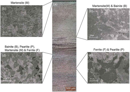
Cross-section of a qualified induction-hardened component is shown in Figure 4. A multi-layered structure is observed in the optical micrograph (Figure 4(a)), where a 4.0-mm-thick light grey layer is at the top, an alternating light-and-dark grey layer in the middle, and a darker feature at the bottom. In addition to the morphology study via SEM observation by backscattered electron (BSE) imaging, microstructure of these layers reveals to have pure martensite (Figure 4(b), i.e. 0.0 mm, at the uppermost surface), a mixture of martensite and bainite (Figure 4(c), i.e. 2.0 mm deep, upper part of the alternating layer), a mixture which dominates with bainite and pearlite, together with ferrite and martensite (Figure 4(d), i.e. 4.0 mm deep, lower part of the alternating layer), and a mixture of pearlite and ferrite (Figure 4(e), i.e. 5.0 mm deep, below the alternating layer), respectively. The average length of the needle-shape martensite reduces from around 40 µm to around 20 µm when going along from the top surface to the 1.0 mm case depth (comparing Figure 4(a, b)). At 2.0 mm depth, bainite starts to develop at the grain boundary with the size smaller than 5 µm (i.e. grain consists of alternating thick light and dark bands) (Figure 4(c)), and then grows to 10–20 µm along the depth. Around 4.0 mm, pearlite (i.e. grains consist of alternating thin light-and-dark grey layers) and ferrite (i.e. clear dark grains) starts to develop (Figure 4d). At the same depth, it is observed that the size of martensite reduces significantly and this microconstituent becomes featureless. Below 5.0 mm, martensite completely disappears, and the grain sizes of pearlite and ferrite are determined to vary between 10 µm and 40 µm (Figure 4(e)). At 7.0 mm, the pearlite size is 75 µm in average. The development of different microconstituents along the cross-section agree with a modelled layered structure that reported earlier based on descending cooling rate [23]. In addition, the micrograph set in Figure 4 confirms that, besides the fast-quenched uppermost martensite layer, no other layer underneath consists of single microconstituent. The mixture of different microconstituents in different depth zone implies that the generated MBN signal is contributed by a matter of varying composition with mixed physical properties. Besides microstructure, the magnetic properties of individual microconstituent depend on the alloy composition [19,26,27], morphology [27], present and amount of precipitates [28,29], grain size [30], internal stress [30], lattice distortion [31] and dislocation density [20,21] according to literature [19–22,26-34]. The acquired BN signal is an integral about all these. In production, it is difficult to have all these factors, together with the case depth, well under controlled. Thus, the data scattering in Figure 2 is understandable. Nevertheless, further discussion related to these topics is not within the scope of present study.

Figure 4. Cross-sectional metallography of a qualified induction-hardened component: (a) an optical micrograph; (b) the uppermost martensite layer (0.0 – ~1.0 mm deep); (c) the mixed martensite and bainite in the upper alternating layer (~2.0 mm deep); (d) the mixed bainite, pearlite, martensite and ferrite in the low alternating layer (~4.0 mm deep); (e) the pearlite-ferrite inner core (~5.0 mm deep)

4. Structural characterisation

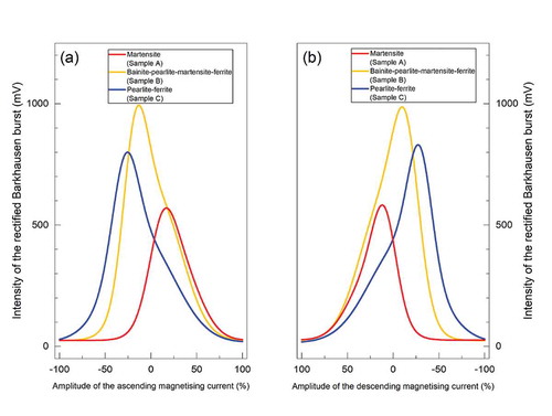
For the multi-layered cross section with mixed microconstituents described above, a preliminary study about the Barkhausen bursts from individual structured layer becomes favourable. A set of 3 sample pieces (dimension: 20 mm × 15 mm × 5 mm) from the raw material were prepared separately. Samples were austenised in a tube furnace at 870°C for 10 minutes, and then quenched/cooled at different rates to imitate the forming conditions of the uppermost martensite layer (Sample A, i.e. quenched in 10 % salt water), the middle bainite-pearlite dominating mixture layer (Sample B, i.e. quenched in a 450 °C salt bath) and the inner pearlite-ferrite core (Sample C, i.e. air-cooled) [23]. Their microstructures are comparable to Figure 4(b, d, e), respectively. Their corresponding rectified Barkhausen bursts are presented in Figure 5. Different microconstituents generate different burst profiles under the same magnetic stimulation in terms of peak intensity, RMS, peak position and FWHM. Sample A shows a relatively low peak intensity and the burst peak locates at a relatively high position. The Samples B and C give higher peak intensity at lower peak position. The low peak intensity of martensite in Sample A, besides the low relative magnetic permeability (µ_r), depends also on the grain size, shape and the dislocation density. Martensite that contains maximum 0.5 wt.% carbon has a rather high pinning site density (e.g. grain boundary), high domain wall density, lattice distortion and high dislocation density, and limited mean free path for the domain movement. Barkhausen noise generation and propagation within the structure is physically hindered. The high domain wall density, together with a high dislocation density, needs more energy to drive the domain motion, thus the corresponding peak position is high [20,21]. Slower transformation rate for bainite formation allows carbon diffusion from the austenitic matrix. The corresponding bainitic-ferrite has lower carbon content and ease the domain wall movement for more intense MBN generation, i.e. peak intensity. This also facilitates lower activation energy for domain nucleation and domain motion, i.e. a relatively lower peak position [20,21]. With the slowest cooling rate, more effective carbon diffusion from austenite to the pro-eutectoid ferrite and then the ferrite-cementite pearlitic lamellar allows the formation of low carbon content ferrite that contains the least dislocation density and align with the cementite at the ease axis. Therefore, the resistance from domain wall energy is the lowest and has the longest mean-free path for domain wall motion. Consequently, it gives the highest peak intensity and the lowest peak position [20,21]. Besides peak intensity and peak position, it is worth to note that the burst shape for Sample A is the narrowest and more symmetric than the other two samples. Asymmetric bursts in Samples B and C can be explained by the multi-microconstituent condition. The mixture of four phases in Sample B gives the broadest burst among three. It has a main peak and a shoulder at the higher position. The main peak locates at a position lower than Sample A, and the shoulder locates around the martensitic position. This implies that the burst of Sample B is mainly contributed by martensite and other microconstituent(s). The FWHM of the Sample C lies at the middle among three. It has a peak at the lowest position and with a shoulder around ‘zero’ position, implying that it also composes of two microconstituents, but neither is martensite. Still, authors should note that a more precise characterisation for ‘non-martensite’, i.e. to distinguish bainite, ferrite and pearlite, based on the current Barkhausen burst analysis is limited.

Figure 5. The smoothened envelopes of the rectified Barkhausen bursts obtained during (a) ascending magnetic field excitation and (b) descending magnetic field excitation of the CF53N steel in different heat-treated forms, i.e. pure martensite (Sample A), the bainite-pearlite-martensite-ferrite mixture (Sample B) and the pearlite-ferrite mixture (Sample C)

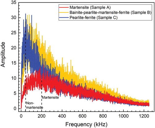
For the inadequacy of Barkhausen burst, electric pulse height of the acquired MBN signal and the MBN amplitude-frequency spectrum are added to help the phase identification. The pulse height distribution in Figure 6 shows that the pure martensite in Sample A gives the majority pulse height peaked at around 30 mV and those from the non-martensitic Sample B and C gives 20 mV. This result is understandable as martensite needs stronger driving force to generate the Barkhausen noise. The amplitude-frequency spectra in Figure 7 shows that frequency range of Sample A (pure martensite) peaks from 200 kHz, while that of Samples B and C (non-martensite) is below 40 kHz, which is in agreement with what Dupois and Saquet has reported [3,4]. Thereby, with the Barkhausen burst, the pulse height distribution plot and the amplitude-frequency spectra, MBN technique can clearly distinguish martensite from the other microconstituents. However, to further identify the type of the non-martensitic phases of this specific steel is still not possible, unless a mono-microconstituent sample of each type can be prepared. Nonetheless, as martensite is the key microconstituent in our case depth study, current finding is enough to proof the presence of the martensitic hardened case and exclude the non-martensitic types. With that, we can keep the valid data for case depth evaluation in the multivariable statistics study.

Figure 6. Pulse height distribution of the MBN signals from pure martensite (Sample A), the mixed bainite-pearlite-martensite-ferrite (Sample B) and the mixed pearlite-ferrite (Sample C)

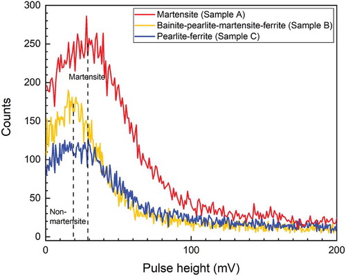
Figure 7. Amplitude spectra from the MBN measurements from pure martensite (Sample A), the mixed bainite-pearlite-martensite-ferrite (Sample B) and the mixed pearlite-ferrite (Sample C)

5. Case depth evaluation

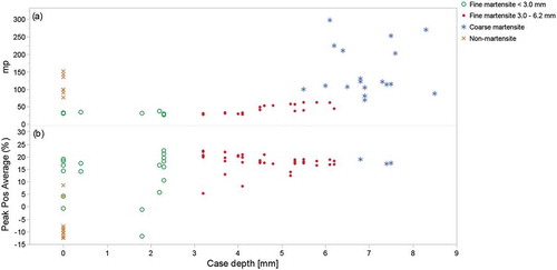
With the above understanding, structural characterisation of the induction-hardened cam lobes based on MBN can be conducted. Characteristic features of the Barkhausen burst including peak intensity, RMS, FWHM and peak position on different measured positions from one of the 17 shafts are studied. The quality of the surface finishing is divided into four categories. They are non-martensite (×), fine martensite < 3.0 mm (ο), fine martensite 3.0–6.0 mm (∙) and coarse martensite (*), as commented in Table 2. Their relationship with mp is presented in Figure 8(a). When focusing on the two qualified conditions, that is the fine martensite with grains smaller than 50 μm, they give a relatively low mp and high burst peak position, as shown Figure 8(a, b). In addition, it is observed that mp are lower for the thinner group, i.e. fine martensite < 3.0 mm. Still, it is difficult to use mp alone to further identify the fine martensite layer with thickness between 0.0 mm and 3.0 mm. Beyond 3.0 mm, an incremental trend is seen in the mp plot (Figure 8(a)). For the coarse martensite with the grains longer than 50 μm, the larger size and lower dislocation density give relatively high mp and high peak position. For non-martensite, mp spreads across low and high level, and the peak position is relatively low. Therefore, by observing both mp and the Barkhausen burst peak position, the four categories can basically be distinguished. Table 3 summarises the observation of parametric variations for each microstructural category. The peak positions in ascending and descending magnetic excitation are at juxtaposition, which means the magnetising and demagnetising mechanisms are rather consistent. FWHM in the non-martensite group is much wider than the other two, and that means multi-microconstituents lead to Barkhausen burst broadening.

Table 2. Classification of different surface conditions after the induction hardening process

Surface conditions	Criteria
Coarse martensite (×)	Surface layer consists of martensite alone, and the average grain size is > 50 µm
Fine martensite < 3 mm (o)	Surface layer consists of martensite alone, and the average grain size is < 50 µm, with case depth less than 3 mm below and at lower specification limit (LSL)
Fine martensite 3–6 mm (∙)	Surface layer consists of martensite alone, and the average grain size is < 50 µm, with case depth 3–6 mm and within specification range
Non-martensite (*)	Surface layer do not consist of martensite only, but mixtures of martensite, bainite, pearlite and ferrite

Table 3. Parametric features of the Barkhausen measurements from different induction-hardened surface conditions

	Coarse martensite (×)	Fine martensite in layer between 3.0–6.0 mm thick (∙)	Fine martensite in layer < 3.0 mm thick (o)	Non-martensite (*)
Case depth (mm)	> 6.0	3.0–6.0	0.0–2.5	0.0–2.0
mp	115–130	30–60	25–35	30–130
RMS (mV)	450–600	100–400	90–170	200–800
FWHM of the burst (%)	30–35	30–45	35–45	45–65
Peak position in the burst during ascending magnetic field excitation (%)	16–18	14–22	16–21	9 – −11
Peak position in the burst during descending magnetic field excitation (%)	17–19	17–22	16–23	10 – −12
Average peak position in the bursts (%)	16–19	14–22	16–23	10 – −10

Figure 8. Plots of case depth vs. (a) mp and (b) the peak position of the Barkhausen burst stratify on microstructural classifications

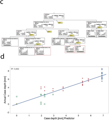
The statistical decision tree modelling [24] is based on random sectioning the data into two sub-sets using the partition platform in the JMP Pro® software. The sub-sets are referring to a training set and a validation set for model building and verification, and contain 75 % and 25 % of the data, respectively (Figure 9). After splitting the data set by seven steps in the decision tree analysis, Figure 10(a) shows the statistical overview of the results. It shows that the R-square (R²) reaches a maximum level at 80 % in the validation set, in which the peak position contributes most to the prediction of case depth by explaining 60% of the case depth variation, the second most influential variable comes mp which explains around one-third of the portion, and the last 8 % is explained by RMS. Figure 10(b) summaries the decision tree analysis. It shows that the qualified condition after induction hardening, i.e. fine martensite structure with the case depth range of 3.0–6.2 mm, can be split into three sub-groups. The averaged case depths of each are 3.76 mm, 5.33 mm and 5.80 mm (i.e. the three red dotted sub-groups in Figure 10b), respectively, in response to the decision criteria (DC) 3, 5 and 6 (Figure 10(b, c)), and Table 4). Figure 10(c) visualises a decision tree that identifies and separates the case depth in ranges for each microstructural class with the statistical figures. In the qualified zone, i.e. the red dots groups, the difference between the lower sub-group and the upper two is also seen in Figure 8, in which a vague but distinct change of mp just above a case depth of 4.0 mm. The predictive plot in Figure 10(d) shows that the precision of case depth prediction from the decision tree model is high when it is > 3.5 mm, where the model correctly predicts both the microstructure and the case depth. The model becomes less accurate in the range around 2.0–3.0 mm whereas several MBN characteristics are found overlapping. Making decision for case depth in the range from 0.0–2.5 mm sometimes are mis-classified, as can be seen in Figure 10(d). Still, the model is conservative in the sense that it predicts case depths above 3.5 mm as it is, but the prediction of 2.0 mm can span from very thin to 4.0 mm in reality. This implies that there is a risk of releasing a bad product (false positive), but the chance is lower than scraping a good one (false negative). The strength of the decision tree classification model lay on its capability to identify local interactions between the MBN characteristics. These characteristics, on the other hand, are driven by the shifting MBN response with reference to the changing microstructure profile overlying the change of case depths as the above described.

Table 4. Decision criteria (DC) based on the Barkhausen burst characteristics for induction-hardened surface classification

Decisioncriteria (DC)	Leaf label	Average case depth [mm]	Count
1	12.4 ≤ Peak Pos Average (%) < 19.54 and mp < 37.8	1.97	9
2	Peak Pos Average (%) ≥ 21.1 and mp <37.8	2.94	5
3	19.54 ≤ Peak Pos Average (%) < 21.1 and mp < 37.8	3.76	7
4	Peak Pos Average (%) ≥ 12.4 and mp ≥ 37.8 and RMS ≥ 467.85	6.90	12
5	Peak Pos Average (%) ≥ 12.4 and RMS < 467.85 and 37.8 ≤ mp < 61.8	5.33	11
6	Peak Pos Average (%) ≥ 12.4 and RMS < 467.85 and 61.8 ≤ mp	5.80	5
7	Peak Pos Average (%) < 12.4 and RMS ≥ 150.52	0.00	14
8	Peak Pos Average (%) < 12.4 and RMS < 150.52	2.26	5

Figure 9. Data splitted into two random sub-sets, i.e. training (75 %) and validation (25 %), for statistical modelling

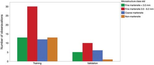
Figure 10. Results of the regression decision tree analysis using the partition platform in JMP Pro®. (a) A statistical overview after 7 splits; (b) summary of the decision tree model; (c) statistical figures of each branch in the decision tree model; (d) a predictive plot of the induction-hardened case depth based on the decision tree model

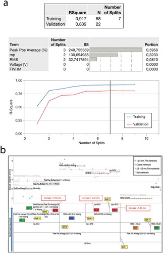
Figure 10. (Continued)

6. Layer uniformity

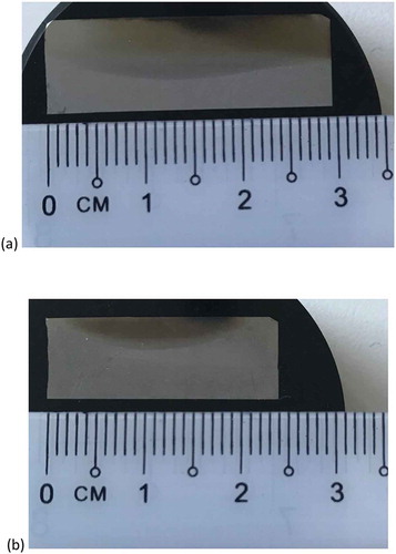
Figure 11 shows the cross-sections of the surface finishing of selected lobes. While most of the components have a uniform hardened layer as in Figure 11(a), non-uniform shape in Figure 11(b) is occasionally found. This non-uniformity will induce a jump in mp and alert warning in production. However, the routine procedure contains insufficient information to evaluate the case depth at this localised region. Another issue about the non-uniform layer thickness is that, if the size of the Barkhausen probe is too large, it covers more than one structural region. The signal interference among the binary, ternary or even quaternary phases can increase complexity in the burst pattern and lead to confusion in structural determination and data analysis.

Figure 11. Cross-section morphology of induction-hardened layer with different finishing: (a) uniform layer; (b) non-uniform layer

7. Physical modelling

Results from the plain numerical simulation model presented in Figure 12(a) shows that the mp for martensite is about half level of bainite, which is shown in both computed flux and the measured mp. The material parameters, used for computing the response of a bilayer model that consists of martensite on top of bainite, comes from the JMatPro® simulations as described in [23]. The two different material layers are then treated as homogenous materials, defined by their corresponding material parameters. Magnetic flux predictions on the top surface show that the flux density decreases when the martensite thickness increases up to 3.0 mm. This agrees with the experimental observation and shows that the computed field affects deeper than the standard depth of penetration (SDP) of 1.6 mm [1,14,23] with the magnetising condition in the industrial practice, i.e. 10 V and 125 Hz.

Figure 12. Comparison between (a) the COMSOL numerical model and (b) the in-line data

Comparing Figure 12(a) to the values in Table 3, it shows a fundamental agreement. Non-martensite shows a higher mp than fine martensite (i.e. case depth 3.0–6.0 mm). In the computation, this corresponds to the material parameters for bainite and martensite, respectively. According to Table 3, coarse martensite (case depth > 6.0 mm) shows a higher mp, but this has no correspondence in the computations. A martensite layer thicker than 3.0 mm, in this computational model, does not contribute any signal increment.

The deviation between Figure 12(a, b), for the case depth of more than 6.0 mm (coarse martensite), could be explained by the current physical model if different sets of material data for fine martensite and coarse martensite had been used. Figure 8 shows that coarse martensite yields a larger experimental mp response than fine martensite, it is then suitable to assume that fine and coarse martensite could have different magnetic properties. However, JMatPro® simulations predict the same permeability and conductivity for both martensitic types, and thus has limited the current development of the physical model.

Figure 8 explains some behaviour in Figure 12(a) for the case depth range 0.0–4.0 mm. Observations in production data (i.e. mp) for shallow case depth deviate from the corresponding numerical flux predictions when it comes to the microstructure that classified as fine martensite. The points that classified as non-martensite, in Figure 8, agree better with the numerical prediction for small case depth, which is reasonable. A martensitic layer of thickness close to 0.0 mm ought to produce a higher mp. Here it is important, with Figure 10(b, d) in mind, to notice the difficulties for classifying between fine martensite of thickness close to 0.0 mm and non-martensite, three samples are incorrectly classified as fine martensite when case depth is 0.0 mm. Figure 10(b) reveals that one of them really belongs to the non-martensite and the two others probably has a case depth > 0.0 mm after all. Thereby, the classification of surfaces that close to case depth < 1.0 mm needs to be studied further.

The deviation between Figure 12(a, b), for the case depth close to 0.0 mm (fine martensite), could then be explained by the difficulties in conducting microstructure classification and thus determining the corresponding depth.

The relationships between case depth and different material parameters are complex. The current numerical model also lacks the possibility to model some physical material behaviour, such as hysteresis. But now, the lack of physical data of the material is believed to be the major shortcoming.

The observed differences in Figure 12 could also, to some extent, be influenced by the fact of the cylindrical geometry of the experimental samples or the actual geometry of the probe. In order to investigate this a model with cylindrical geometry needs to be made, this is however out of the scope of this paper.

8. Conclusions

Case depth of the martensitic induction-hardened surface layer with grain size smaller than 50 µm on the CF53N camshaft lobes is investigated by means of magnetic Barkhausen noise (MBN) method in an industrial practice. By investigating the routine monitored mp reading, together with the Barkhausen burst features including RMS of peak intensity and peak position, the microstructural characteristics of this desired process-hardened layer can be identified, i.e. mp 20–70, peak position 16–23% and RMS 100–400 mV. Then, case depth evaluation of this qualified condition can be conducted with the aid of multivariable statistical modelling. Regression decision tree model can help to categorise this qualified condition with the case depth range between 3.0 and 6.2 mm into three sub-groups that averaged at 3.76 mm, 5.33 mm and 5.80 mm. Still, a more precise determination of case depth is restricted. Therefore, the numerical results from MBN measurements and statistical multivariable analysis show that this method is feasible, but advanced physical modelling will be needed to improve the scientific validity.

Acknowledgements

Authors acknowledge the financial support from the Sweden’s Innovation Agency (VINNOVA) in the Non-destructive Characterization Concepts for Production project (FFI-OFP4p) between November 2015 and November 2018. Authors gratefully acknowledge the co-partnership with Mr. Jonas Holmberg, Dr. Albin Stormvinter and Mr. Pär Andersson in RISE IVF AB (Former Swerea IVF AB) and Mr. Per Lundin in Schlumpf Scandinavia AB during the project development.

Disclosure statement

No potential conflict of interest was reported by the author(s).

Additional information

Funding

This work was supported by the VINNOVA [2015-03721 FFI OFP4p].

References

- Jiles DC. Review of magnetic methods for non-destructive evaluation. NDT Int. 1988;21(5):311–319.
- Bach G, Goebbels K, Theiner WA. Characterization of hardening depth by Barkhausen noise measurement. Mater Eval. 1988;46:1576–1580.
- Dubois M, Fiset M. Evaluation of case depth on steels by Barkhausen noise measurement. Mater Sci Technol. 1995;11(3):264–267.
- Saquet O, Tapuleasa D, Chicois J. Use of Barkhausen noise for determination of surface hardened depth. Nondestruct Test Eval. 1998;14(5):277–292. .
- Vaidyanathan S, Moorthy V, Jayakumar T, et al. Evaluation of induction hardened case depth through microstructural characterisation using magnetic Barkhausen emission technique. Mater Sci Technol. 2000;26(2):202–208.
- Blaow M, Evans JT, Shaw BA. Effect of hardness and composition gradients on Barkhausen emission in case hardened steel. J Magn Magn Mater. 2006;303(1):153–159.
- Lo CCH, Kinser ER, Melikhov Y, et al. Magnetic non-destructive characterization of case depth in surface-hardened steel components. In: Thompson DO, Chimenti DE, editors. Quantitative non-destructive evaluation. 2005 Jul 31 – Aug 5. Brunswick, Maine (USA): AIP Conference Proceedings; 2006. Vol. 82. p. 1253–1260.
- Zhang C, Bowler N, Lo C. Magnetic characterization of surface-hardened steel, J. Magn Magn Mater. 2009;321(23):3878–3887.
- Kobayashi S, Takahashi H, Kamada Y. Evaluation of case depth in induction-hardened steels: magnetic hysteresis measurements and hardness-depth profiling by differential permeability analysis. J Magn Magn Mater. 2013;343:112–118.
- Santa-Aho S, Vippola M, Sorsa A, et al. Utilization of Barkhausen noise magnetizing sweeps for case-depth detection from hardened steel. NDT E Int. 2012;52:95–102.
- Kahrobaee S, Hejazi T-H, Akhlaghi IA. Electromagnetic methods to improve the non-destructive characterization of induction hardened steels: A statistical modeling approach. Surf Coat Technol. 2019;380:125074.
- Stresstech Group. Microscan 600 Operating instructions, V.5.4b; 2015.
- Stresstech Oy. Stresscan 500C Operating instructions, V.1.0; 2002.
- Stresstech Group. Rollscan 350 Operating instructions, V 2.0; 2016.
- Tiitto S Magnetoelastic testing of uniaxial and biaxial stresses. In: Beck G, Denis S, Simon A, editors. Proceedings of the Second International conference on residual stresses (ICRS2); 1988 Nov 23-25; Nancy, France. Springer, Dordrecht, 1989. p. 234–240.
- Magalas LB. Application of the wavelet transform in mechanical spectroscopy and in Barkhausen noise analysis. J Alloys Compd. 2000;310(1–2):269–275.
- Ceurter JS, Smith C, Ott R The Barkhausen noise inspection method for detecting grinding damage in gears. In: Proceedings of the second international conference on Barkhausen noise and micromagnetic testing (ICBM2); 1999 Oct 25-26; Newcastle, UK. p. 91–100.
- Spike (action potential) activity burst fitting [Internet]. New York (NY): Cornell University; [cited 2019 Oct 16]. Available from: https://people.ece.cornell.edu/land/PROJECTS/BurstFit/index.html
- Gür CH. Characterization of steel microstructures by magnetic Barkhausen noise technique. In: Güneş O, Akkaya Y, editors. Non-destructive Testing of Materials and Structures. Vol. 6. RILEM Book series ed. Dordrecht: Springer; 2013. p. 449–504.
- Saquet O, Chicois J, Vincent A. Barkhausen noise from plain carbon steels: analysis of the influence of microstructure. Mater Sci Eng A. 1999;269(1–2):73–82.
- Clapman L, Jagadish C, Atherton DL. The influence of pearlite on Barkhausen noise generation in plain carbon steels. Acta Mater. 1991;39(7):1555–1562.
- Tam PL, Persson G, Hammersberg P, et al. Preliminary Study: Barkhausen noise evaluation on the hardening depth of induction-hardened carbon steel. In: Suortti-Suominen T, editor. Conference proceedings in the twelfth international conference on Barkhausen noise and micromagnetic testing (ICBM12); 2017 Sep 25-26; Dresden, Germany. Finland, Stresstech Oy; p. 73–83.
- Grayson J, Gardner S, Stephens M. Building better models with JMP pro. Cary, NC: SAS Institute Inc.; 2005.
- Persson G On the modelling of a Barkhausen sensor. The twelfth European conference on the Non-destructive Testing (ECNDT 2018); 2018 Jun 11-15; Gothenburg, Sweden. NDT.net Issue 2018-8, http://www.ndt.net/?id=22841
- Chin GY, Wernick JH. Soft magnetic metallic materials. In: Wohlfarth EP, editor. Ferromagnetic materials – handbook. Vol. 2. Elsevier; 1980. p. 55–188.
- Jiles DC. Magnetic properties and microstructure of AISI 1000 series carbon steels. J Phys D App Phys. 1988;21(7):1186–1195.
- Kameda J, Ranjan R. Non-destructive evaluation of steels using acoustic and magnetic Barkhausen signals – I. Effect of carbide precipitation and hardness. Acta Mater. 1987;35(7):1515–1526.
- Kameda J, Ranjan R. Non-destructive evaluation of steels using acoustic and magnetic Barkhausen signals – II. Effect of intergranular impurity segregation. Acta Mater. 1987;35(7):1527–1531.
- Anglada-Rivera J, Padovese LR, Capó-Sánchez J. Magnetic Barkhausen noise and hysteresis loop in commercial carbon steel: influence of applied tensile stress and grain size. J Magn Magn Mater. 2001;231(2–3):299–306.
- Blaow M, Evans JT, Shaw BA. Magnetic Barkhausen noise: the influence of microstructure and deformation in bending. Acta Mater. 2005;53(2):279–287.
- Stupakov O, Pal’a J, Yurchenko V, et al. Measurement of Barkhausen noise and its correlation with magnetic permeability. J Magn Magn Mater. 2008;320(3–4):204–209. .
- Bida GV, Nichipuruk AP, Tsar´kova TP. Magnetic properties of steels after quenching and tempering. I General. Carbon steel. Russ J Nondestruct. 2001;37(2):79–99. .
- Moorthy V. Important factors influencing the magnetic Barkhausen noise profile. IEEE Trans Magn. 2016;52(4):6200713.