
ABSTRACT
The flow in a large section (80%) of an Advanced Gas-cooled Reactor fuel assembly is investigated in two configurations, the former dealing with the fuel assembly operating in normal plant conditions and the latter with a cold gas injected sideways at the top of Element 2 of the fuel assembly. Results show that injecting the cold gas decreases the temperature at the top of the assembly and that mixing is almost complete there.
KEYWORDS:
1. Introduction
Extending the current nuclear power plant lifetime is crucial to cover the ever-growing energy demand, before renewable energy gets more widespread and affordable. Checks and measurements carried out during plant operation provide necessary data to ensure safe operation, but in order to understand the changes after many years of service, a more detailed knowledge of the working conditions inside the reactor is needed. New measurements are not possible without costly intrusive and disruptive work on site. Meanwhile, the constant improvement of computational fluid dynamics (CFD) and high-performance computing (HPC) has made them suitable to tackle complex issues occurring in industrial situations.
An Advanced Gas-cooled Reactor (AGR) fuel element contains 36 fuel pins that hold the fuel pellets (see ). The 36 fuel pins are contained within a cylindrical graphite sleeve. The fuel pins have helical ribs in order to increase the rate of heat transfer from the pins and to improve gas mixing in the fuel cluster (see ). A fuel assembly is made out of eight such fuel elements, stacked vertically end to end. As the graphite bricks are making up the core of the reactor age, there is a possibility that mechanical interaction between the graphite sleeves and the bricks could cause small axial gaps to open between the fuel element sleeves. The gap could allow ingress of gas at a different temperature to occur. Currently, it is assumed that all gas mixes before reaching the top of the assembly, due to the swirling motion imposed by the helical ribs. Recent studies using CFD have shown that the effect of the ribs might be limited to a region close to the pins, and therefore it is possible that the two streams of cold and hot gas do not mix completely before exiting the assembly.
Figure 1. AGR fuel element.
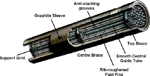
Figure 2. Close-up of the ribbed pins.
The temperature at the end of the assembly is measured by a single thermocouple and thus it is impossible to know from plant data how uniform the thermal field is. In order to see what the effect of ingress of gas at a given point is, a CFD calculation is carried out. Due to the temperature distribution on the sleeve and the fuel pins, the thermal field evolves as the gas goes upwards. This means that a periodic calculation can only predict the pressure drop but not the thermal field. A CFD calculation involving the whole assembly has never been tried before due to the large number of cells required to mesh this domain, i.e. 1.6 billion cells in the present case.
Section 2 presents the geometry dealt with; Section 3 presents some features of Code_Saturne; Section 4 presents the performance of Code_Saturne on a Blue Gene/Q; Section 5 presents the results obtained for the cases without and with cold gas injection, before concluding in Section 6.
2. Geometry
The AGR fuel assembly is made of eight elements and each of them have 36 pins. A guide tube in the middle of each element goes through all the way to the top of the assembly and its surface is smooth. A gap exists between each element to allow the pins to expand when heated. The pins are helically ribbed with 12 starts. An element contains a mixture of right-handed and left-handed helices to promote gas mixing. This means that symmetry is only achieved for 120° sectors. Unlike the real element, the model does not contain any braces or support grids.
The effect of gas ingress from the top of Element 2 is investigated in this study. Therefore, the model starts at the middle of Element 2 and contains all the 6.5 elements located on top of it. The computed configuration goes from about 1.5 to 8 m. All the 36 pins of the assembly and the guide tube in its centre are accounted for.
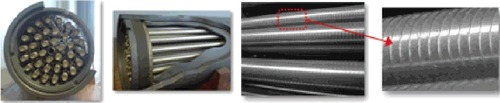
Two main parts of the model might be meshed independently, the elements including the fuel pins and the gaps between each element, respectively. In order to create the mesh for the pins, a repeatable base section of a length equivalent to the rib pitch is created (see ). This section contains about 5.4 million tetrahedral cells. The capability of Code_Saturne for gluing meshes is used to translate and join this section 30 times. This creates one fuel element. Another mesh of about 2.1 million prismatic cells is generated for the gap between elements. It is glued at the top of each element using the CFD software. This process is repeated 6.5 times to create the domain made of 6.5 elements. All the interfaces are carefully constructed as conformal, even though Code_Saturne can handle non-conformal joining. This avoids creating extra faces and saves CPU time. The mesh of the gap is built by extracting the boundary face of the base unit mesh, filling the holes for the pins surfaces and extruding it in the vertical direction with refinement near the pins. A prism layer is added to all the solid surfaces of the full mesh. The total number of cells for the 6.5-meter element mesh is 1,068,926,189.
Figure 3. Fuel pin mesh. Left: repeatable base section. Right: ribs on the pins and their absence for the guide tube.

3. Numerical approach
The CFD software Code_Saturne (Archambeau, Mechitoua, and Sakiz Citation2004) is used to compute the flow inside the fuel assembly. It is an open-source CFD software package based on the finite volume method that can handle any type of mesh built with any cell/grid structure. Incompressible and compressible flows can be simulated, with or without heat transfer, and a range of turbulence models is available. Parallelism is handled by distributing the domain over the processors and communication between subdomains through message passing interface (MPI). Hybrid parallelism using OpenMP has recently been added for improved multicore performance, but is not used in this work.
The recent developments of the code to join or glue meshes in parallel are exploited to obtain the full domain mesh directly on the machine where the calculation takes place.The turbulence model used is the SST model (Menter Citation1994) with wall functions. The working fluid is CO2 and its properties have been made function of the temperature. The boundary conditions have been taken from a representative set for normal operation of an AGR. These include the inlet velocities and temperatures at the middle of Element 2 and the heat flux profiles of the graphite sleeve and heat from the nuclear fuel (both functions of the height).
4. Performance
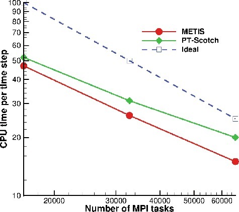
An IBM Blue Gene/Q hosted by STFC at the Hartree Centre has been used to perform the simulations. It has six racks of 1,024 nodes, each node (16 GB RAM) being made of 16 physical cores. Hyperthreading using up to 64 threads per node is possible. Code_Saturne has been optimised in recent years for high-end machines (Fournier et al. Citation2011) and has already shown good performance up to 1,572,864 MPI tasks of DOE Argonne's Blue Gene/Q. shows the time to solution as a function of the number of MPI tasks (16,384 to 65,536), using METIS or PT-Scotch as partitioners. Linear performance is observed in both cases, but METIS produces a better partition for Code_Saturne, as the time per time step is much smaller than when PT-Scotch is used.
Figure 4. Example of Code_Saturne scalability on a Blue Gene/Q. Serial METIS and PT-Scotch are used as partitioners.
gathers the time for IOs for a typical simulation on the Blue Gene/Q using 512 nodes and 32 ranks per node (hyperthreading for 16,384 MPI tasks). The Blue Gene/Q uses a GPFS system and MPI-IO handles IOs in the code.
Table 1. Blue Gene/Q simulation using 512 nodes and 32 ranks per node (16,384 cores). The mesh is made of 1,068,926,189 cells.
5. Results
Two calculations are presented in this paper. The first one computes the flow inside a large section (80%) of the AGR fuel assembly operating in normal conditions. It is used as a basis for comparison. The second case has the same domain, mesh and boundary conditions but a colder gas is injected at the top of Element 2. This represents what might occur when the graphite sleeves move leading to the creation of a space in the locking system. The injection area is obtained by selecting faces of the sleeve located in a circle. The injection velocity and temperature are imposed. In real plant conditions, the shape of the injection might not be circular, but for the purpose of this study, the shape is not expected to have a large influence on the results. The mass flow rate of the jet is about 9% of the mass flow rate in the assembly. The bulk velocity of the jet is about 1.8 times larger than the averaged inlet velocity at the bottom of the domain.
The base case presents some level of mixing of the gas as it travels upwards. The helical ribs induce a swirl that enhances the heat transfer at the pins but also helps mixing between the different channels between the ribs. The swirl generated by the ribs is clearly observed in (left) at the top of Element 2.
Figure 5. Streamlines. Left: at the top of Element 2. Right: from the injection boundary.
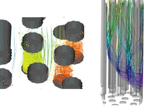
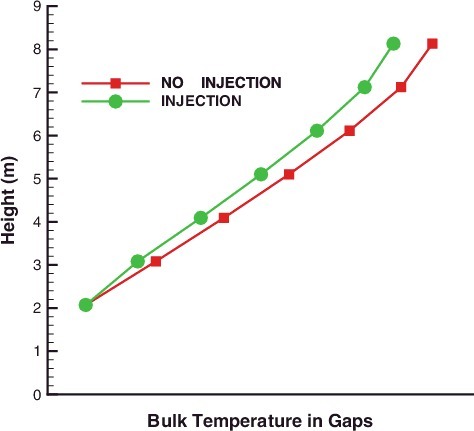
The injection section is presented in (right) where the streamlines are plotted. It can be seen that most of the flow bends upwards before reaching the centre of the assembly. Temperature contours in horizontal planes at each gap between the elements are shown for both cases in . The temperature has been normalised by the bulk temperature at each gap in order to enable a better comparison. It can be seen that, as the gas travels upwards, the colder gas gets mixed. This pattern is observed up to Gap 6 (top of Element 7). At the outlet (Gap 7, top of Element 8), mixing is almost complete. The bulk temperature at each of the gaps between the elements is shown in for both cases. As expected, the cold gas injection reduces the total temperature of the gas in the assembly.
Figure 6. Normalised temperature at each gap (Top: Gap 1). Left: case without injection. Right: case with injection.
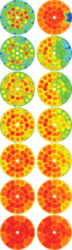
Figure 7. Bulk temperature at each gap.
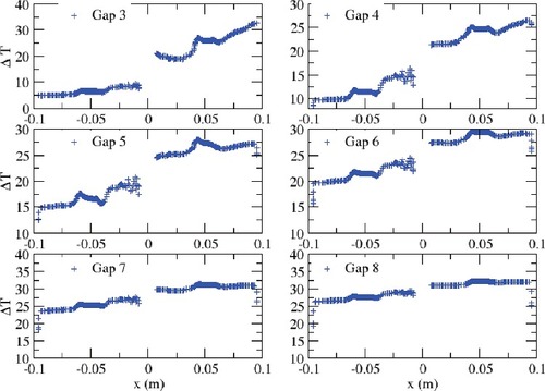
In order to be able to compare how much of the gas is mixed, profiles of temperature difference (base case minus injection case) are plotted in . The x-coordinate represents the distance from the centre of the assembly and the y-coordinate the second horizontal coordinate. The injection is located at (x, y) = (10−1, 0). Therefore, for each profile, the side on the positive x is where the injection is located. The gap on the curve is due to the guide tube, which is not heated. It can be seen that the difference between both sides is large at the gap between Elements 3 and 4 (Gap 3) because the injection is set just above Gap 2. By the time the flow reaches Gap 8, the difference between both sides is greatly reduced. This suggests that for the conditions given in this case, there is enough mixing of the gas before the outlet boundary to consider the effect of the injection as homogeneous. For other cases where the injection would be located above Element 2 or set using a different mass flow rate, this might not be true. Comparisons with a single-point temperature as given by the only available thermocouple are certainly not representative. It is noted that the thermocouple is not located at Element 8 but further downstream beyond the neutron scatter plug, top reflector and flow control gag, which might generate additional mixing. Their influence on the flow will have to be investigated further.
Figure 8. Temperature difference between both cases.
6. Conclusions
The flow inside the AGR fuel assembly has been computed. The large size of the domain and the need to resolve the detail around the ribs make it necessary to use a code that has excellent HPC performance. Code_Saturne has been selected for these reasons and the recent improvements on its HPC capabilities have been tested here for a real industrial case. The code has demonstrated excellent performance and issues encountered by processing a large amount of data have been solved using the tools available inside the code.
The flow in the assembly operating in normal plant conditions has been compared with a case where a cold gas is injected through the graphite sleeve. For this particular case, the computation shows that mixing is almost complete when reaching the last fuel element. It is important to note that for other scenarios where the sleeve leakage would occur at a higher position or with a different mass flow rate, a cold plume might still be present by the time the gas reaches the end of Element 8. This should be investigated further.
Acknowledgements
The authors would like to thank the Hartree Centre for using Blue Joule, their Blue Gene/Q. An award of computer time was provided by the Innovative and Novel Computational Impact on Theory and Experiment (INCITE) program. This research used resources of the Argonne Leadership Computing Facility, which is a DOE Office of Science User Facility supported under Contract DE-AC02-06CH11357.
Disclosure statement
No potential conflict of interest was reported by the authors.
Additional information
Funding
References
- Archambeau, F., N. Mechitoua, and M. Sakiz. 2004. “A Finite Volume Method for the Computation of Turbulent Incompressible Flows – Industrial Applications.” International Journal on Finite Volumes 1(1): 1–62.
- Fournier, Y., J. Bonelle, C. Moulinec, Z. Shang, A.G. Sunderland, and J.C. Uribe. 2011. “Optimizing Code_Saturne Computations on Petascale Systems.” Computers & Fluids 45: 103–108.
- Menter, F. 1994. “Two-Equation Eddy-Viscosity Turbulence Models for Engineering Applications.” AIAA Journal 32: 1598–1605.