A Measure of Directional Outlyingness With Applications to Image Data and Video

ABSTRACT

Functional data analysis covers a wide range of data types. They all have in common that the observed objects are functions of a univariate argument (e.g., time or wavelength) or a multivariate argument (say, a spatial position). These functions take on values which can in turn be univariate (such as the absorbance level) or multivariate (such as the red/green/blue color levels of an image). In practice it is important to be able to detect outliers in such data. For this purpose we introduce a new measure of outlyingness that we compute at each gridpoint of the functions’ domain. The proposed directional outlyingness (DO) measure accounts for skewness in the data and only requires $\mathcal{O}\left(n\right)$ computation time per direction. We derive the influence function of the DO and compute a cutoff for outlier detection. The resulting heatmap and functional outlier map reflect local and global outlyingness of a function. To illustrate the performance of the method on real data it is applied to spectra, MRI images, and video surveillance data.

KEYWORDS:

• Functional data
• Influence function
• Outlier detection
• Robustness
• Skewness

1. Introduction

Functional data analysis (Ramsay and Silverman 2005; Ferraty and Vieu 2006) is a rapidly growing research area. Often the focus is on functions with a univariate domain, such as time series or spectra. The function values may be multivariate, such as temperatures measured at 3, 9, and 12 cm below ground (Berrendero, Justel, and Svarc 2011) or human ECG data measured at eight different places on the body (Pigoli and Sangalli 2012). In this article we will also consider functions whose domain is multivariate. In particular, images and surfaces are functions on a bivariate domain. Our methods generalize to higher-dimensional domains, for example the voxels of a three-dimensional image of a human brain are defined on a trivariate domain.

Detecting outliers in functional data is an important task. Recent developments include the approaches of Febrero-Bande, Galeano, and González-Manteiga (2008) and Hyndman and Shang (2010). Sun and Genton (2011) proposed the functional boxplot, and Arribas-Gil et al. (2014) developed the outliergram. Our approach is somewhat different. To detect outlying functions or outlying parts of a function (in a dataset consisting of several functions) we will look at its (possibly multivariate) function value in every time point/pixel/voxel/... of its domain. For this purpose we need a tool that assigns a measure of outlyingness to every data point in a multivariate nonfunctional sample. A popular measure is the Stahel-Donoho outlyingness (SDO) due to Stahel (1981) and Donoho (1982) which works best when the distribution of the inliers is roughly elliptical. However, it is less suited for skewed data. To address this issue, Brys, Hubert, and Rousseeuw (2005) proposed the (skewness-) adjusted outlyingness (AO) which takes the skewness of the underlying distribution into account. However, the AO has two drawbacks. The first is that the AO scale has a large bias as soon as the contamination fraction exceeds 10%. Furthermore, its computation time is $\mathcal{O}(nlog(n\left)\right)$ per direction due to its rather involved construction.

To remedy these deficiencies we propose a new measure in this article, the directional outlyingness (DO). The DO also takes the skewness of the underlying distribution into account, by the intuitive idea of splitting a univariate dataset in two half samples around the median. The AO incorporates a more robust scale estimator, which requires only $\mathcal{O}\left(n\right)$ operations.

Section 2 defines the DO, investigates its theoretical properties, and illustrates it on univariate, bivariate, and spectral data. Section 3 derives a cutoff value for the DO and applies it to outlier detection. It also extends the functional outlier map of Hubert, Rousseeuw, and Segaert (2015) to the DO, and in it constructs a curve separating outliers from inliers. Section 4 shows an application to MRI images, and Section 5 analyzes video data. Section 6 contains simulations in various settings, to study the behavior of DO and compare its performance to other methods. Section 7 concludes.

2. A Notion of Directional Outlyingness

2.1. Univariate Setting

In the univariate setting, the Stahel-Donoho outlyingness of a point y relative to a sample Y = {y₁, …, y_n} is defined as (1) $$\text{SDO}(y;Y)=\frac{|y-\text{med}(Y\left)\right|}{\text{MAD}\left(Y\right)},$$(1) where the denominator is the median absolute deviation (MAD) of the sample, given by $\text{MAD}\left(Y\right)={\text{med}}_i\left(\right|y_i-{\text{med}}_j\left(y_j\right)\left|\right)/{\Phi }^{-1}(0.75)$ where Φ is the standard normal cdf. The SDO is affine invariant, meaning that it remains the same when a constant is added to Y and y, and also when they are multiplied by a nonzero constant.

A limitation of the SDO is that it implicitly assumes the inliers (i.e., the nonoutliers) to be roughly symmetrically distributed. But when the inliers have a skewed distribution, using the MAD as a single measure of scale does not capture the asymmetry. For instance, when the data stem from a right-skewed distribution, the SDO may become large for inliers on the right-hand side, and not large enough for actual outliers on the left-hand side.

This observation led to the (skewness-) adjusted outlyingness (AO) proposed by Brys, Hubert, and Rousseeuw (2005). This notion employs a robust measure of skewness called the medcouple (Brys, Hubert, and Struyf 2004), which however requires $\mathcal{O}(nlog(n\left)\right)$ computation time. Moreover, we will see in the next subsection that it leads to a rather large explosion bias.

In this article we propose the notion of directional outlyingness (DO) which also takes the potential skewness of the underlying distribution into account, while attaining a smaller computation time and bias. The main idea is to split the sample into two half samples, and then to apply a robust scale estimator to each of them.

More precisely, let y₁ ⩽ y₂ ⩽ ⋅⋅⋅ ⩽ y_n be a univariate sample. (The actual algorithm does not require sorting the data.) We then construct two subsamples of size $h=⌊\frac{n+1}{2}⌋$ as follows. For even n we take Y_a = {y_{h + 1}, …, y_n} and Y_b = {y₁, …, y_h} where the subscripts a and b stand for above and below the median. For odd n we put Y_a = {y_h, …, y_n} and Y_b = {y₁, …, y_h} so that Y_a and Y_b share one data point and have the same size.

Next, we compute a scale estimate for each subsample. Among many available robust estimators we choose a one-step M-estimator with Huber ρ-function due to its fast computation and favorable properties. We first compute initial scale estimates $$\begin{array}{ccc}\hfill {\text{s}}_{o,a}\left(Y\right)& =& \text{med}\left(Z_a\right)/{\Phi }^{-1}(0.75)\text{and}\hfill \\ \hfill {\text{s}}_{o,b}\left(Y\right)& =& \text{med}\left(Z_b\right)/{\Phi }^{-1}(0.75),\hfill \end{array}$$where $Z_a=Y_a-\text{med}\left(Y\right)$ and $Z_b=\text{med}\left(Y\right)-Y_b$ and where Φ^{− 1}(0.75) ensures consistency for Gaussian data. The one-step M-estimates are then given by (2) $$\begin{array}{ccc}\hfill {\text{s}}_a\left(Y\right)& =& {\text{s}}_{o,a}\left(Y\right)\sqrt{\frac{1}{2\alpha h}{\sum }_{z_i\in Z_a}{\rho }_c\left(\frac{z_i}{{\text{s}}_{o,a}\left(Y\right)}\right)}\hfill \\ \hfill {\text{s}}_b\left(Y\right)& =& {\text{s}}_{o,b}\left(Y\right)\sqrt{\frac{1}{2\alpha h}{\sum }_{z_i\in Z_b}{\rho }_c\left(\frac{z_i}{{\text{s}}_{o,b}\left(Y\right)}\right),}\hfill \end{array}$$(2) where again $h=⌊\frac{n+1}{2}⌋$ and where α = ∫^∞₀ρ_c(x)dΦ(x). Here ρ_c denotes the Huber rho function for scale ${\rho }_c\left(t\right)={\left(\frac{t}{c}\right)}^2{\mathbb{1}}_{[-c,c]}+{\mathbb{1}}_{(-\infty ,c)\cup (c,\infty )}$ with c a tuning parameter regulating the trade-off between efficiency and bias.

Finally, the DO of a point y relative to a univariate sample Y = {y₁, …, y_n} is given by (3) $$\text{DO}(y;Y)=\left\{\begin{array}{cc}\hfill \frac{y-\text{med}\left(Y\right)}{{\text{s}}_a\left(Y\right)}& \hfill \text{if}y⩾\text{med}\left(Y\right)\\ \hfill \frac{\text{med}\left(Y\right)-y}{{\text{s}}_b\left(Y\right)}& \hfill \text{if}y⩽\text{med}\left(Y\right).\end{array}\right.$$(3) Note that DO is affine invariant. In particular, flipping the signs of Y and y interchanges s_a and s_b which results in DO( − y; −Y) = DO(y; Y).

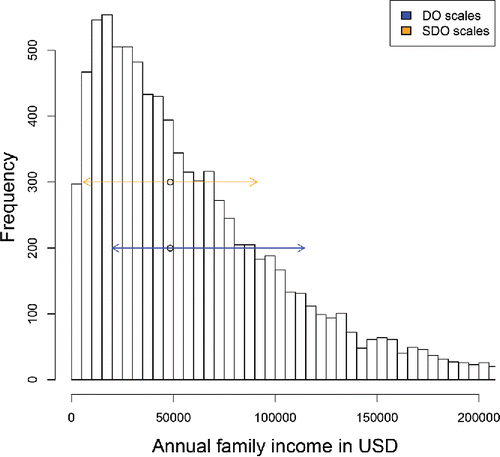
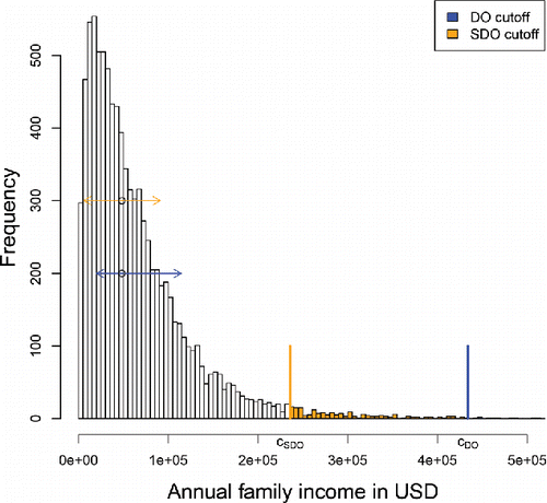
Figure 1 illustrates the denominators of the SDO and DO expressions on the family income dataset from https://psidonline.isr.umich.edu which contains 8962 strictly positive incomes in the tax year 2012. Their histogram is clearly right-skewed. The MAD in the denominator of SDO equals < ent {$ 42, 650 and is used both to the left and to the right of the median, as depicted by the orange arrows. For the DO the “above” scale s_a = <ent {$ 58, 681 exceeds the “below” scale s_b = <ent {$ 35, 737 (blue arrows). Therefore, a point to the right of the median will have a lower DO than a point to the left at the same distance to the median. This is a desirable property in view of the difference between the left and right tails.

Figure 1. Scale estimates of the family income data. The SDO scale is measured symmetrically about the median, whereas the DO scales are not and reflect skewness.

2.2. Robustness Properties

Let us now study the robustness properties of the scales s_a and s_b and the resulting DO. It will be convenient to write s_a and s_b as functionals of the data distribution F: (4) $$\begin{array}{ccc}\hfill {\text{s}}_a^2\left(F\right)& =& \frac{{\text{s}}_{o,a}^2\left(F\right)}{\alpha }{\int }_{\mathrm{med}\left(F\right)}^{\infty }{\rho }_c\left(\frac{x-\text{med}\left(F\right)}{{\text{s}}_{o,a}\left(F\right)}\right)dF\left(x\right)\hfill \\ \hfill {\text{s}}_b^2\left(F\right)& =& \frac{{\text{s}}_{o,b}^2\left(F\right)}{\alpha }{\int }_{-\infty }^{\mathrm{med}\left(F\right)}{\rho }_c\left(\frac{\text{med}\left(F\right)-x}{{\text{s}}_{o,b}\left(F\right)}\right)dF\left(x\right),\hfill \end{array}$$(4) where ρ_c is the Huber ρ-function.

We will first focus on the worst-case bias of s_a due to a fraction ϵ of contamination, following Martin and Zamar (1993). At a given distribution F, the explosion bias curve of s_a is defined as $$B^{+}(\epsilon ,{\text{s}}_a,F)=\underset{G\in {\mathcal{F}}_{\epsilon }}{sup}\left({\text{s}}_a\left(G\right)\right),$$where ${\mathcal{F}}_{\epsilon }=\{G:G=(1-\epsilon )F+\epsilon H\}$ in which H can be any distribution. The implosion bias curve is defined similarly as $$B^{-}(\epsilon ,{\text{s}}_a,F)=\underset{G\in {\mathcal{F}}_{\epsilon }}{inf}\left({\text{s}}_a\left(G\right)\right).$$

From here onward we will assume that F is symmetric about some center m and has a continuous density f(x) which is strictly decreasing in x > m. To derive the explosion and implosion bias we require the following lemma (all proofs can be found in the Appendix):

Lemma 1.

(i)	For fixed μ it holds that $t^2{\int }_{\mu }^{\infty }{\rho }_c\left(\frac{x-\mu }{t}\right)dF\left(x\right)$ is strictly increasing in t > 0.
(ii)	For fixed σ > 0 it holds that ${\sigma }^2{\int }_t^{\infty }{\rho }_c\left(\frac{x-t}{\sigma }\right)dF\left(x\right)$ is strictly decreasing in t.

Proposition 1.

For any 0 < ϵ < 0.25 the implosion bias of s_a is given by $$\begin{array}{ccc}& & B^{-}{(\epsilon ,{\text{s}}_a,F)}^2=\frac{1}{\alpha }{B}^{-}{(\epsilon ,{\text{s}}_{o,a},F)}^2\hfill \\ & & \times \left\{(1-\epsilon ){\int }_{B^{+}(\epsilon ,\text{med},F)}^{\infty }{\rho }_c\left(\frac{x-B^{+}(\epsilon ,\text{med},F)}{B^{-}(\epsilon ,{\text{s}}_{o,a},F)}\right)dF\left(x\right)\right\},\hfill \end{array}$$where $$\begin{array}{ccc}\hfill B^{+}(\epsilon ,\text{med},F)& =& F^{-1}\left(\frac{1}{2(1-\epsilon )}\right)\hfill \\ \hfill B^{-}(\epsilon ,{\text{s}}_{o,a},F)& =& \frac{1}{{\Phi }^{-1}\left(\frac{3}{4}\right)}\left\{F^{-1}\left(\frac{3-4\epsilon }{4(1-\epsilon )}\right)-F^{-1}\left(\frac{1}{2(1-\epsilon )}\right)\right\}.\hfill \end{array}$$

In fact, the implosion bias of s_a is reached when $H=\Delta \left(F^{-1}\left(\frac{1}{2(1-\epsilon )}\right)\right)$ is the distribution that puts all its mass in the point $F^{-1}\left(\frac{1}{2(1-\epsilon )}\right)$. Note that the implosion breakdown value of s_a is 25% because for ϵ → 0.25 we obtain s_a → 0.

Proposition 2.

For any 0 < ϵ < 0.25 the explosion bias of s_a is given by $$\begin{array}{ccc}& & B^{+}{(\epsilon ,{\text{s}}_a,F)}^2=\frac{1}{\alpha }{B}^{+}{(\epsilon ,{\text{s}}_{o,a},F)}^2\hfill \\ & & \times \left\{(1-\epsilon ){\int }_{B^{+}(\epsilon ,\text{med},F)}^{\infty }{\rho }_c\left(\frac{x-B^{+}(\epsilon ,\text{med},F)}{B^{+}(\epsilon ,{\text{s}}_{o,a},F)}\right)dF\left(x\right)+\epsilon \right\},\hfill \end{array}$$where $$\begin{array}{ccc}& & B^{+}(\epsilon ,{\text{s}}_{o,a},F)\hfill \\ & & =\frac{1}{{\Phi }^{-1}\left(\frac{3}{4}\right)}\left\{F^{-1}\left(\frac{3}{4(1-\epsilon )}\right)-F^{-1}\left(\frac{1}{2(1-\epsilon )}\right)\right\}.\hfill \end{array}$$

The explosion bias of s_a is reached at all distributions F_ϵ = (1 − ϵ)F + ϵΔ(d) for which d > B⁺(ϵ, med, F) + cB⁺(ϵ, s_{o, a}, F) which ensures that d lands on the constant part of ρ_c. For ϵ → 0.25 we find d → ∞ and s_a → ∞, so the explosion breakdown value of s_a is 25%.

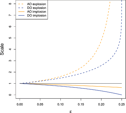
The blue curves in Figure 2 are the explosion and implosion bias curves of s_a when F = Φ is the standard Gaussian distribution, and the tuning constant in ρ_c is c = 2.1 corresponding to 85% efficiency. By affine equivariance the curves for s_b are exactly the same, so these are the curves of both DO scales. The orange curves correspond to explosion and implosion of the scales used in the adjusted outlyingness AO under the same contamination. We see that the AO scale explodes faster, due to using the medcouple in its definition. The fact that the DO scale is typically smaller enables the DO to attain larger values in outliers.

Figure 2. Comparison of explosion and implosion bias of the AO and DO scales.

Another tool to measure the (non-)robustness of a procedure is the influence function (IF). Let T be a statistical functional, and consider the contaminated distribution F_{ϵ, z} = (1 − ϵ)F + ϵΔ(z). The influence function of T at F is then given by $$\text{IF}(z,T,F)=\underset{\epsilon \to 0}{lim}\frac{T\left(F_{\epsilon ,z}\right)-T\left(F\right)}{\epsilon }=\frac{\partial }{\partial \epsilon }T\left(F_{\epsilon ,z}\right){|}_{\epsilon =0}$$and basically describes how T reacts to a small amount of contamination.

This concept justifies our choice for the function ρ_c. Indeed, the IF of a fully iterated M-estimator of scale with function ρ is proportional to ρ(z) − β with the constant β = ∫^∞_{− ∞}ρ(x)dF(x). We use ρ = ρ_c with c = 2.1. It was shown in Hampel et al. (1986) that at F = Φ this ρ_c yields the M-estimator with highest asymptotic efficiency subject to an upper bound on the absolute value of its IF.

We will now derive the IF of the one-step M-estimator s_a given by (4(4) $$\begin{array}{ccc}\hfill {\text{s}}_a^2\left(F\right)& =& \frac{{\text{s}}_{o,a}^2\left(F\right)}{\alpha }{\int }_{\mathrm{med}\left(F\right)}^{\infty }{\rho }_c\left(\frac{x-\text{med}\left(F\right)}{{\text{s}}_{o,a}\left(F\right)}\right)dF\left(x\right)\hfill \\ \hfill {\text{s}}_b^2\left(F\right)& =& \frac{{\text{s}}_{o,b}^2\left(F\right)}{\alpha }{\int }_{-\infty }^{\mathrm{med}\left(F\right)}{\rho }_c\left(\frac{\text{med}\left(F\right)-x}{{\text{s}}_{o,b}\left(F\right)}\right)dF\left(x\right),\hfill \end{array}$$(4) ).

Proposition 3.

The influence function of s_a is given by $$\begin{array}{ccc}& & 2\alpha \frac{{\text{s}}_a\left(F\right)}{{\text{s}}_{o,a}^2\left(F\right)}\text{IF}(z,{\text{s}}_a,F)\hfill \\ & & =\left\{\frac{2}{{\text{s}}_{o,a}\left(F\right)}{\int }_{\text{med}\left(F\right)}^{\infty }{\rho }_c\left(\frac{x-\text{med}\left(F\right)}{{\text{s}}_{o,a}\left(F\right)}\right)dF\left(x\right)\right.\hfill \\ & & -{\int }_{\text{med}\left(F\right)}^{\infty }x{\rho }_c^{\text{'}}\left(\frac{x-\text{med}\left(F\right)}{{\text{s}}_{o,a}\left(F\right)}\right)dF\left(x\right)\hfill \\ & & \left.+\text{med}\left(F\right){\int }_{\text{med}\left(F\right)}^{\infty }{\rho }_c^{\text{'}}\left(\frac{x-\text{med}\left(F\right)}{{\text{s}}_{o,a}\left(F\right)}\right)dF\left(x\right)\right\}\text{IF}(z,{\text{s}}_{o,a},F)\hfill \\ & & -\left\{{\int }_{\text{med}\left(F\right)}^{\infty }{\rho }_c^{\text{'}}\left(\frac{x-\text{med}\left(F\right)}{{\text{s}}_{o,a}\left(F\right)}\right)dF\left(x\right)\right\}\text{IF}(z,\text{med},F)\hfill \\ & & +\left\{{\mathbb{1}}_{\left[\text{med}\right(F),\infty )}\left(z\right){\rho }_c(z-\text{med}\left(F\right))-\alpha \right\},\hfill \end{array}$$where IF(z, s_{o, a}, F) is the influence function of s_{o, a}.

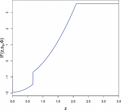
The resulting IF of s_a at F = Φ is shown in Figure 3. [Note that IF(z, s_b, Φ) = IF( − z, s_a, Φ).] It is bounded, indicating that s_a is robust to a small amount of contamination even when it is far away. Note that the IF has a jump at the third quartile Q₃ ≈ 0.674 due to the initial estimate s_{o, a}. If we were to iterate (4(4) $$\begin{array}{ccc}\hfill {\text{s}}_a^2\left(F\right)& =& \frac{{\text{s}}_{o,a}^2\left(F\right)}{\alpha }{\int }_{\mathrm{med}\left(F\right)}^{\infty }{\rho }_c\left(\frac{x-\text{med}\left(F\right)}{{\text{s}}_{o,a}\left(F\right)}\right)dF\left(x\right)\hfill \\ \hfill {\text{s}}_b^2\left(F\right)& =& \frac{{\text{s}}_{o,b}^2\left(F\right)}{\alpha }{\int }_{-\infty }^{\mathrm{med}\left(F\right)}{\rho }_c\left(\frac{\text{med}\left(F\right)-x}{{\text{s}}_{o,b}\left(F\right)}\right)dF\left(x\right),\hfill \end{array}$$(4) ) to convergence this jump would vanish, but then the explosion bias would go up a lot, similarly to the computation in Rousseeuw and Croux (1994).

Figure 3. Influence function of s_a at F = Φ.

Let us now compute the influence function of DO(x; F) given by (3(3) $$\text{DO}(y;Y)=\left\{\begin{array}{cc}\hfill \frac{y-\text{med}\left(Y\right)}{{\text{s}}_a\left(Y\right)}& \hfill \text{if}y⩾\text{med}\left(Y\right)\\ \hfill \frac{\text{med}\left(Y\right)-y}{{\text{s}}_b\left(Y\right)}& \hfill \text{if}y⩽\text{med}\left(Y\right).\end{array}\right.$$(3) ) for contamination in the point z, noting that x and z need not be the same.

Proposition 4.

When $x>\text{med}\left(F\right)$ it holds that $$\begin{array}{ccc}\hfill \text{IF}(z,DO(x),F)& =& \frac{-1}{{\text{s}}_a^2\left(F\right)}\{\text{IF}(z,\text{med},F){\text{s}}_a\left(F\right)\hfill \\ & & +\text{IF}(z,{\text{s}}_a,F)(x-\text{med}\left(F\right))\}\hfill \end{array}$$whereas for x < med(F) we obtain $$\begin{array}{ccc}\hfill \text{IF}(z,DO(x),F)& =& \frac{1}{{\text{s}}_b^2\left(F\right)}\{\text{IF}(z,\text{med},F){\text{s}}_b\left(F\right)\hfill \\ & & -\text{IF}(z,{\text{s}}_b,F)(\text{med}\left(F\right)-x)\}.\hfill \end{array}$$

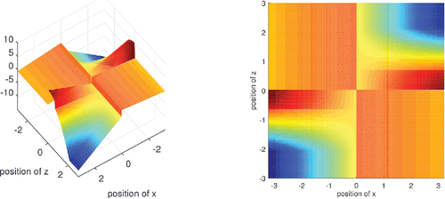
For a fixed value of x the influence function of DO(x) is bounded in z. This is a desirable robustness property. Figure 4 shows the influence function (which is a surface) when F is the standard Gaussian distribution.

Figure 4. Influence function of DO(x) for F = Φ. Left: 3D, right: 2D seen from above. For a fixed point x it is bounded over all possible positions z of contamination.

2.3. Multivariate Setting

In the multivariate setting we can apply the principle that a point is outlying with respect to a dataset if it stands out in at least one direction. Like the Stahel-Donoho outlyingness, the multivariate DO is defined by means of univariate projections. To be precise, the DO of a d-variate point $\mathbf{y}$ relative to a d-variate sample $\mathbf{Y}=\{{\mathbf{y}}_1,\dots ,{\mathbf{y}}_n\}$ is defined as (5) $$\text{DO}(\mathbf{y};\mathbf{Y})=\underset{\mathbf{v}\in {\mathbb{R}}^d}{sup}\text{DO}({\mathbf{y}}^T\mathbf{v};{\mathbf{Y}}^T\mathbf{v}),$$(5) where the right-hand side uses the univariate DO of (3(3) $$\text{DO}(y;Y)=\left\{\begin{array}{cc}\hfill \frac{y-\text{med}\left(Y\right)}{{\text{s}}_a\left(Y\right)}& \hfill \text{if}y⩾\text{med}\left(Y\right)\\ \hfill \frac{\text{med}\left(Y\right)-y}{{\text{s}}_b\left(Y\right)}& \hfill \text{if}y⩽\text{med}\left(Y\right).\end{array}\right.$$(3) ).

To compute the multivariate DO we have to rely on approximate algorithms, as it is impossible to project on all directions $\mathbf{v}$ in d-dimensional space. A popular procedure to generate a direction is to randomly draw d data points, compute the hyperplane passing through them, and then to take the direction $\mathbf{v}$ orthogonal to it. This guarantees that the multivariate DO is affine invariant. That is, the DO does not change when we add a constant vector to the data, or multiply the data by a nonsingular d × d matrix.

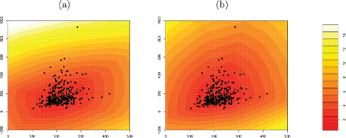
As an illustration we take the bloodfat dataset, which contains plasma cholesterol and plasma triglyceride concentrations (in mg/dl) of 320 male subjects for whom there is evidence of narrowing arteries (Hand et al. 1994). Here n = 320 and d = 2, and following Hubert and Van der Veeken (2008) we generated 250d = 500 directions $\mathbf{v}$. Figure 5 shows the contour plots of both the DO and SDO measures. Their contours are always convex. We see that the contours of the DO capture the skewness in the dataset, whereas those of the SDO are more symmetric even though the data themselves are not.

Figure 5. Bloodfat data with (a) SDO contours, and (b) DO contours. The DO contours better reflect the skewness in the data.

2.4. Functional Directional Outlyingness

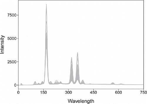
We now extend the DO to data where the objects are functions. To fix ideas we will consider an example. The glass dataset consists of spectra with d = 750 wavelengths resulting from spectroscopy on n = 180 archeological glass samples (Lemberge et al. 2000). Figure 6 shows the 180 curves.

Figure 6. Spectra of 180 archeological glass samples.

At each wavelength the response is a single number, the intensity, so this is a univariate functional dataset. However, we can incorporate the dynamic behavior of these curves by numerically computing their first derivative. This yields bivariate functions, where the response consists of both the intensity and its derivative.

In general we write a functional dataset as $\mathbf{Y}=\{Y_1,Y_2,\dots ,Y_n\}$ where each Y_i is a d-dimensional function. As in this example, the Y_i are typically observed on a discrete set of points in their domain. For a univariate domain this set is denoted as {t₁, …, t_T}.

Now we want to define the DO of a d-variate function X on the same domain, where X need not be one of the Y_i. For this we look at all the domain points t_j in turn, and define the functional directional outlyingness (fDO) of X with respect to the sample Y as (6) $$\text{fDO}(X;\mathbf{Y})=\sum _{j=1}^T\text{DO}(X\left(t_j\right);\mathbf{Y}\left(t_j\right))W\left(t_j\right),$$(6) where W(.) is a weight function for which ∑^T_{j = 1}W(t_j) = 1. Such a weight function allows us to assign a different importance to the outlyingness of a curve at different domain points. For instance, one could downweight time points near the boundaries if measurements are recorded less accurately at the beginning and the end of the process.

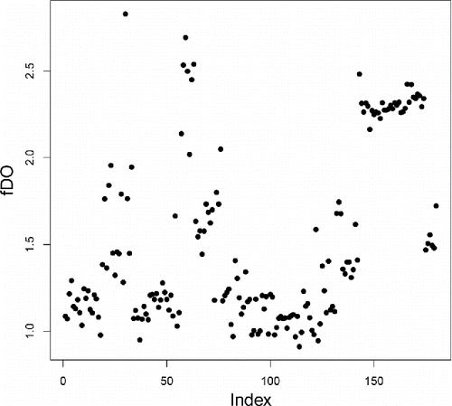
Figure 7 shows the fDO of the 180 bivariate functions in the glass data, where W(.) was set to zero for the first 13 wavelengths where the spectra had no variability, and constant at the remaining wavelengths. These fDO values allow us to rank the spectra from most to least outlying, but do not contain much information about how the outlying curves are different from the majority.

Figure 7. Functional DO (fDO) values of the 180 glass spectra. Higher fDO values correspond to curves that are more outlying on average.

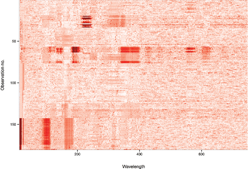
In addition to this global outlyingness measure fDO we also want to look at the local outlyingness. To this end Figure 8 shows the individual $\text{DO}(Y_i\left(t_j\right);\mathbf{Y}\left(t_j\right))$ for each of the 180 functions Y_i of the glass data at each wavelength t_j. Higher values of DO are shown by darker red in this heatmap. Now we see that there are a few groups of curves with particular anomalies: one group around function 25, one around function 60, and one with functions near the bottom. Note that the global outlyingness measure fDO flags outlying rows in this heatmap, whereas the dark spots inside the heatmap can be seen as outlying cells. It is also possible to sort the rows of the heatmap according to their fDO values. Note that the wavelength at which a dark spot in the heatmap occurs allows to identify the chemical element responsible.

Figure 8. Heatmap of DO of the glass data. Darker pixels indicate outlying behavior.

As in Hubert, Rousseeuw, and Segaert (2015) we can transform the DO to the multivariate depth function 1/(DO + 1), and the fDO to the functional depth function 1/(fDO + 1).

3. Outlier Detection

3.1. A Cutoff for Directional Outlyingness

When analyzing a real dataset we do not know its underlying distribution, but still we would like a rough indication of which observations should be flagged as outliers. For this purpose we need an approximate cutoff value on the DO. We first consider non-functional data, leaving the functional case for the next subsection. Let $\mathbf{Y}=\{{\mathbf{y}}_1,\dots ,{\mathbf{y}}_n\}$ be a d-variate dataset (d ⩾ 1) with directional outlyingness values {DO₁, …, DO_n}. The DO_i have a right-skewed distribution, so we transform them to {LDO₁, …, LDO_n} = {log (0.1 + DO₁), …, log (0.1 + DO_n)} of which the majority is closer to Gaussian. Then we center and normalize the resulting values in a robust way and compare them to a high gaussian quantile. For instance, we can flag ${\mathbf{y}}_i$ as outlying whenever (7) $$\frac{{\text{LDO}}_i-\text{med}\left(\text{LDO}\right)}{\text{MAD}\left(\text{LDO}\right)}>{\Phi }^{-1}(0.995),$$(7) so the cutoff for the DO values is $c=\text{exp}(\text{med}\left(LDO\right)+\text{MAD}\left(LDO\right){\Phi }^{-1}(0.995))-0.1$. (Note that we can use the same formulas for functional data by replacing DO by fDO.)

For an illustration we return to the family income data of Figure 1. The blue vertical line in Figure 9 corresponds to the DO cutoff, whereas the orange line is the result of the same computation applied to the SDO. The DO cutoff is the more conservative one, because it takes the skewness of the income distribution into account.

Figure 9. Outlier cutoffs for the family income data. The DO-based cutoff takes the data skewness into account.

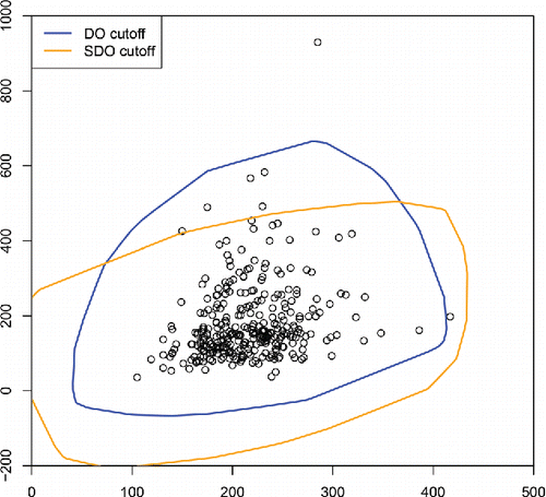
Figure 10 shows the DO and SDO cutoffs for the bivariate bloodfat data of Figure 5. The DO captures the skewness in the data and flags only two points as outlying, whereas the SDO takes a more symmetric view and also flags five of the presumed inliers.

Figure 10. Outlier detection on bloodfat data. The DO-based cutoff adapts to the data skewness and flags fewer points as outlying.

3.2. The Functional Outlier Map

When the dataset consists of functions there can be several types of outlyingness. As an aid to distinguish between them, Hubert, Rousseeuw, and Segaert (2015) introduced a graphical tool called the functional outlier map (FOM). Here we will extend the FOM to the new DO measure and add a cutoff to it, to increase its utility.

Consider a functional dataset $\mathbf{Y}=\{Y_1,Y_2,\dots ,Y_n\}$. The fDO [see (6(6) $$\text{fDO}(X;\mathbf{Y})=\sum _{j=1}^T\text{DO}(X\left(t_j\right);\mathbf{Y}\left(t_j\right))W\left(t_j\right),$$(6) )] of a function Y_i can be interpreted as the “average outlyingness” of its (possibly multivariate) function values. We now also measure the variability of its DO values, by (8) $$\text{vDO}(Y_i;\mathit{Y})=\frac{{\text{stdev}}_j\left(\text{DO}(Y_i\left(t_j\right);\mathbf{Y}\left(t_j\right))\right)}{1+\text{fDO}(Y_i;\mathbf{Y})}.$$(8) Note that (8(8) $$\text{vDO}(Y_i;\mathit{Y})=\frac{{\text{stdev}}_j\left(\text{DO}(Y_i\left(t_j\right);\mathbf{Y}\left(t_j\right))\right)}{1+\text{fDO}(Y_i;\mathbf{Y})}.$$(8) ) has the fDO in the denominator to measure relative instead of absolute variability. This can be understood as follows. Suppose that the functions Y_i are centered around zero and that Y_k(t_j) = 2Y_i(t_j) for all j. Then ${\text{stdev}}_j\left(\text{DO}(Y_k\left(t_j\right);\mathbf{Y}\left(t_j\right))\right)=2{\text{stdev}}_j\left(\text{DO}(Y_i\left(t_j\right);\mathbf{Y}\left(t_j\right))\right)$ but their relative variability is the same. Because $\text{fDO}(Y_k;\mathbf{Y})=2\text{fDO}(Y_i;\mathbf{Y})$, putting fDO in the denominator normalizes for this. In the numerator we could also compute a weighted standard deviation with the weights W(t_j) from (6(6) $$\text{fDO}(X;\mathbf{Y})=\sum _{j=1}^T\text{DO}(X\left(t_j\right);\mathbf{Y}\left(t_j\right))W\left(t_j\right),$$(6) ).

The FOM is then the scatterplot of the points (9) $$\left(\text{fDO}(Y_i;\mathit{Y}),\text{vDO}(Y_i;\mathit{Y})\right)$$(9) for i = 1, …, n. Its goal is to reveal outliers in the data, and its interpretation is fairly straightforward. Points in the lower left part of the FOM represent regular functions which hold a central position in the dataset. Points in the lower right part are functions with a high fDO but a low variability of DO values. This happens for shift outliers, that is, functions which have a regular shape but are shifted on the whole domain. Points in the upper left part have a low fDO but a high vDO. Typical examples are local outliers, that is functions which only display outlyingness over a small part of their domain. The points in the upper right part of the FOM have both a high fDO and a high vDO. These correspond to functions which are strongly outlying on a substantial part of their domain.

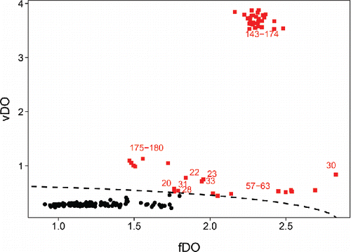
As an illustration we revisit the glass data. Their FOM in Figure 11 contains a lot more information than their fDO values alone in Figure 7. In the heatmap (Figure 8) we noticed three groups of outliers, which also stand out in the FOM. The first group consists of the spectra 20, 22, 23, 28, 30, 31, and 33. Among these, number 30 lies furthest to the right in the FOM. It corresponds to row 30 in Figure 8 which has a dark red piece. It does not look like a shift outlier, for which the row would have a more homogeneous color (hence a lower vDO). The second group, with functions 57–63, occupies a similar position in the FOM. The group standing out the most consists of functions 143–174. They are situated in the upper part of the FOM, indicating that they are shape outliers. Indeed, they deviate strongly from the majority in three fairly small series of wavelengths. Their outlyingness is thus more local than that of functions 57–63.

Figure 11. Functional outlier map (FOM) of the glass data, with cutoff curve.

We now add a new feature to the FOM, namely a rule to flag outliers. For this we define the combined functional outlyingness (CFO) of a function Y_i as (10) $$\begin{array}{ccc}\hfill {\text{CFO}}_i& =& \text{CFO}(Y_i;\mathit{Y})\hfill \\ & =& \sqrt{{({\text{fDO}}_i/\text{med}\left(\text{fDO}\right))}^2+{({\text{vDO}}_i/\text{med}\left(\text{vDO}\right))}^2},\hfill \end{array}$$(10) where ${\text{fDO}}_i=\text{fDO}(Y_i;\mathit{Y})$ and $\text{med}\left(\text{fDO}\right)=\text{med}({\text{fDO}}_1,\dots ,{\text{fDO}}_n)$, and similarly for vDO. Note that the CFO characterizes the points in the FOM through their Euclidean distance to the origin, after scaling. We expect outliers to have a large CFO. In general, the distribution of the CFO is unknown but skewed to the right. To construct a cutoff for CFO we use the same reasoning as for the cutoff (7(7) $$\frac{{\text{LDO}}_i-\text{med}\left(\text{LDO}\right)}{\text{MAD}\left(\text{LDO}\right)}>{\Phi }^{-1}(0.995),$$(7) ) on fDO: First we compute ${\text{LCFO}}_i=log(0.1+{\text{CFO}}_i)$ for all i = 1, …, n, and then we flag function Y_i as outlying if (11) $$\frac{{\text{LCFO}}_i-\text{med}\left(\text{LCFO}\right)}{\text{MAD}\left(\text{LCFO}\right)}>{\Phi }^{-1}(0.995).$$(11) This yields the dashed curve (which is part of an ellipse) in the FOM of Figure 11.

4. Application to Image Data

Images are functions on a bivariate domain. In practice the domain is a grid of discrete points, for example the horizontal and vertical pixels of an image. It is convenient to use two indices j = 1, …, J and k = 1, …, K, one for each dimension of the grid, to characterize these points. An image (or a surface) is then a function on the J × K points of the grid. Note that the function values can be univariate, like gray intensities, but they can also be multivariate, for example the intensities of red, green, and blue (RGB). In general we will write an image dataset as a sample $\mathbf{Y}=\{Y_1,Y_2,\dots ,Y_n\}$ where each Y_i is a function from {(j, k); j = 1, …, J and k = 1, …, K} to ${\mathbb{R}}^d$.

The fDO (6(6) $$\text{fDO}(X;\mathbf{Y})=\sum _{j=1}^T\text{DO}(X\left(t_j\right);\mathbf{Y}\left(t_j\right))W\left(t_j\right),$$(6) ) and vDO (8(8) $$\text{vDO}(Y_i;\mathit{Y})=\frac{{\text{stdev}}_j\left(\text{DO}(Y_i\left(t_j\right);\mathbf{Y}\left(t_j\right))\right)}{1+\text{fDO}(Y_i;\mathbf{Y})}.$$(8) ) notions that we saw for functional data with a univariate domain can easily be extended to functions with a bivariate domain by computing (12) $$\text{fDO}(Y_i;\mathbf{Y})=\sum _{j=1}^J\sum _{k=1}^K\text{DO}(Y_i(j,k);\mathbf{Y}(j,k))W_{jk},$$(12) where the weights W_jk must satisfy ∑^J_{j = 1}∑_{k = 1}^KW_jk = 1, and (13) $$\text{vDO}(Y_i;\mathbf{Y})=\frac{{\text{stdev}}_{j,k}\left(\text{DO}(Y_i(j,k);\mathbf{Y}(j,k))\right)}{1+\text{fDO}(Y_i;\mathbf{Y})},$$(13) where the standard deviation can also be weighted by the W_jk. (The simplest weight function is the constant W_jk = 1/(JK) for all j = 1, …, J and k = 1, …, K.) Note that (12(12) $$\text{fDO}(Y_i;\mathbf{Y})=\sum _{j=1}^J\sum _{k=1}^K\text{DO}(Y_i(j,k);\mathbf{Y}(j,k))W_{jk},$$(12) ) and (13(13) $$\text{vDO}(Y_i;\mathbf{Y})=\frac{{\text{stdev}}_{j,k}\left(\text{DO}(Y_i(j,k);\mathbf{Y}(j,k))\right)}{1+\text{fDO}(Y_i;\mathbf{Y})},$$(13) ) can trivially be extended to functions with domains in more than 2 dimensions, such as three-dimensional images consisting of voxels. In each case we obtain fDO_i and vDO_i values that we can plot in a FOM, with cutoff value (11(11) $$\frac{{\text{LCFO}}_i-\text{med}\left(\text{LCFO}\right)}{\text{MAD}\left(\text{LCFO}\right)}>{\Phi }^{-1}(0.995).$$(11) ).

As an illustration we analyze a dataset containing MRI brain images of 416 subjects aged between 18 and 96 (Marcus et al. 2007), which can be freely accessed at www.oasis-brains.org. For each subject several images are provided; we will use the masked atlas-registered gain field-corrected images resampled to 1mm isotropic pixels. The masking has set all non-brain pixels to an intensity value of zero. The provided images are already normalized, meaning that the size of the head is exactly the same in each image. The images have 176 by 208 pixels, with grayscale values between 0 and 255. All together we thus have 416 observed images Y_i containing univariate intensity values Y_i(j, k), where j = 1, …, J = 176 and k = 1, …, K = 208.

There is more information in such an image than just the raw values. We can incorporate shape information by computing the gradient in every pixel of the image. The gradient in pixel (j, k) is defined as the two-dimensional vector $\nabla Y_i(j,k)=(\frac{\partial Y_i(j,k)}{\partial j},\frac{\partial Y_i(j,k)}{\partial k})$ in which the derivatives have to be approximated numerically. In the pixels at the boundary of the brain we compute forward and backward finite differences, and for the other pixels we employ central differences. In the horizontal direction we thus compute one of three expressions: $$\begin{array}{ccc}\hfill & & \frac{\partial Y_i(j,k)}{\partial j}\hfill \\ & & =\left\{\begin{array}{c}\hfill (-3Y_i(j,k)+4Y_i(j+1,k)\\ \hfill -Y_i(j+2,k))/2& \hfill \left(\text{forward}\text{difference}\right)\\ \hfill (Y_i(j+1,k)-Y_i(j-1,k))/2& \hfill \left(\text{central}\text{difference}\right)\\ \hfill (Y_i(j-2,k)-4Y_i(j-1,k)\\ \hfill +3Y_i(j,k))/2& \hfill \left(\text{backward}\text{difference}\right)\end{array}\right.\hfill \end{array}$$depending on where the pixel is located. The derivatives in the vertical direction are computed analogously.

Incorporating these derivatives yields a dataset of dimensions 416 × 176 × 208 × 3, so the final Y_i(j, k) are trivariate. For each subject we thus have three data matrices which represent the original MRI image and its derivatives in both directions. Figure 12 shows these three matrices for subject number 387.

Figure 12. Original MRI image of subject 387, and its derivatives in the horizontal and vertical direction.

The functional DO of an MRI image Y_i is given by (12(12) $$\text{fDO}(Y_i;\mathbf{Y})=\sum _{j=1}^J\sum _{k=1}^K\text{DO}(Y_i(j,k);\mathbf{Y}(j,k))W_{jk},$$(12) ): $$\text{fDO}(Y_i;\mathbf{Y})=\frac{1}{176\times 208}\sum _{j=1}^{176}\sum _{k=1}^{208}\text{DO}(Y_i(j,k);\mathbf{Y}(j,k))W_{jk},$$where $\text{DO}(Y_i(j,k);\mathbf{Y}(j,k))$ is the DO of the trivariate point Y_i(j, k) relative to the trivariate dataset {Y₁(j, k), …, Y₄₁₆(j, k)}. In this example, we have set the weight W_jk equal to zero at the grid points that are not part of the brain, shown as the black pixels around it. The grid points inside the brain receive full weight.

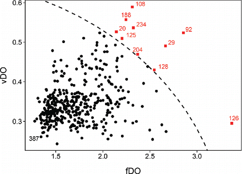
Figure 13 shows the resulting FOM, which indicates the presence of several outliers. Image 126 has the highest fDO combined with a relatively low vDO. This suggests a shift outlier, that is, a function whose values are all shifted relative to the majority of the data. Images 29 and 92 have a large fDO in combination with a high vDO, indicating that they have strongly outlying subdomains. Images 108, 188, and 234 have an fDO which is on the high end relative to the dataset, which by itself does not make them outlying. Only in combination with their large vDO are they flagged as outliers. These images have strongly outlying subdomains which are smaller that those of functions 29 and 92. The remaining flagged images are fairly close to the cutoff, meaning they are merely borderline cases.

Figure 13. Functional outlier map (FOM) of the MRI dataset, with cutoff curve.

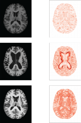
To find out why a particular image is outlying it is instructive to look at a heatmap of its DO values. In Figure 14 we compare the MRI images (on the left) and the DO heatmaps (on the right) of subjects 387, 92, and 126. DO values of 15 or higher received the darkest color. Image 387 has the smallest CFO value, and can be thought of as the most central image in the dataset. As expected, the DO heatmap of image 387 shows very few outlying pixels. For subject 92, the DO heatmap nicely marks the region in which the MRI image deviates most from the majority of the images. Note that the boundaries of this region have the highest outlyingness. This is due to including the derivatives in the analysis, as they emphasize the pixels at which the grayscale intensity changes. The DO heatmap of subject 126 does not show any extremely outlying region but has a rather high outlyingness over the whole domain, which explains its large fDO and regular vDO value. The actual MRI image to its left is globally lighter than the others, confirming that it is a shift outlier.

Figure 14. MRI image (left) and DO heatmap (right) of subjects 387 (top), 92 (middle), and 126 (bottom).

5. Application to Video

We analyze a surveillance video of a beach, filmed with a static camera (Li et al. 2004). This dataset can be found at http://perception.i2r.a-star.edu.sg/bk_model/bk_index.html and consists of 633 frames.

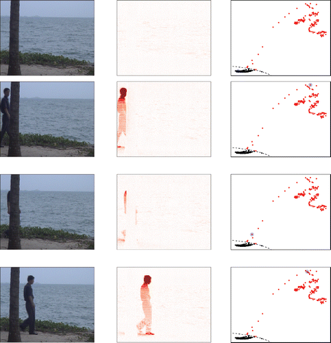
The first 8 seconds of the video show a beach with a tree, as in the leftmost panel of Figure 15. Then a man enters the screen from the left (second panel), disappears behind the tree (third panel), and then reappears to the right of the tree and stays on screen until the end of the video. The frames have 160 × 128 pixels and are stored using the RGB (Red, Green and Blue) color model, so each frame corresponds to three matrices of size 160 × 128. Overall we have 633 frames Y_i containing trivariate Y_i(j, k) for j = 1, …, J = 160 and k = 1, …, K = 128.

Figure 15. Frames number 100, 487, 491, and 500 from the video dataset.

Computing the fDO (12(12) $$\text{fDO}(Y_i;\mathbf{Y})=\sum _{j=1}^J\sum _{k=1}^K\text{DO}(Y_i(j,k);\mathbf{Y}(j,k))W_{jk},$$(12) ) in this dataset is time consuming since we have to execute the projection pursuit algorithm (5(5) $$\text{DO}(\mathbf{y};\mathbf{Y})=\underset{\mathbf{v}\in {\mathbb{R}}^d}{sup}\text{DO}({\mathbf{y}}^T\mathbf{v};{\mathbf{Y}}^T\mathbf{v}),$$(5) ) in ${\mathbb{R}}^3$ for each pixel, so 160 × 128 = 20, 480 times. The entire computation took 25 minutes on a laptop. Therefore we switch to an alternative computation. We define the componentwise DO of a d-variate point $\mathbf{y}$ relative to a d-variate sample $\mathbf{Y}=\{{\mathbf{y}}_1,\dots ,{\mathbf{y}}_n\}$ as (14) $$\text{CDO}(\mathbf{y};\mathbf{Y})=\sqrt{{\sum }_{h=1}^d\text{DO}{(y_h;Y_h)}^2},$$(14) where DO(y_h; Y_h) is the univariate DO of the h-th coordinate of $\mathbf{y}$ relative to the h th coordinate of $\mathbf{Y}$. 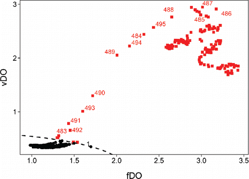Analyzing the video data with this componentwise procedure took 15 seconds, so it is a 100 times faster than with projection pursuit, and it produced almost the same FOM. Figure 16 shows the FOM obtained from the CDO computation.

Figure 16. Functional outlier map of the video data.

The first 480 frames, which depict the beach and the tree with only the ocean surface moving slightly, are found at the bottom left part of the FOM. They fall inside the dashed curve that separates the regular frames from the outliers. At frame 483 the man enters the picture, making the standard deviation of the DO rise slightly. The fDO increases more slowly, as the fraction of the pixels covered by the man is still low at this stage. This frame can thus be seen as locally outlying. The subsequent frames 484–487 have very high fDO and vDO. In them the man is clearly visible between the left border of the frame and the tree, so these frames have outlying pixels in a substantial part of their domain. Frames 489–492 see the man disappear behind the tree, so the fDO goes down as the fraction of outlying pixels decreases. From frame 493 onward the man reappears to the right of the tree and stays on screen until the end. These frames contain many outlying pixels, yielding points in the upper right part of the FOM.

In the FOM we also labeled frame 1, which lies close to the outlyingness border. Further inspection indicated that this frame is a bit lighter than the others, which might be due to the initialization of the camera at the start of the video.

In addition to the FOM we can draw DO heatmaps of the individual frames. For frames 100, 487, 491, and 500, Figure 17 shows the raw frame on the left, the DO heatmap in the middle and the FOM on the right, in which a blue circle marks the position of the frame. In this figure we can follow the man's path in the FOM, while the DO heatmaps show exactly where the man is in those frames. We have created a video in which the raw frame, the DO heatmap and the FOM evolve alongside each other. It can be downloaded from http://wis.kuleuven.be/stat/robust/papers-since-2010.

Figure 17. Left: Frames 100, 487, 491, and 500 from the video. Middle: DO heatmaps of these frames. Right: FOM with blue marker at the position of the frame.

6. Simulation Study

We would also like to study the performance of the DO when the data generating mechanism is known, and compare it with the AO measure proposed by Brys, Hubert, and Rousseeuw (2005) and studied by Hubert and Van der Veeken (2008) and Hubert, Rousseeuw, and Segaert (2015). For this we carried out an extensive simulation study, covering univariate as well as multivariate and functional data.

In the univariate case we generated m = 1000 standard lognormal samples of size n = {200, 500, 1000} with 10% and 15% of outliers at the position x, which may be negative. Figure 18 shows the effect of the contamination at x on our figure of merit, the percentage of outliers flagged (averaged over the m replications).

Figure 18. Percentage of outliers found in univariate lognormal samples of size n = 200 (left), n = 500 (middle), and n = 1000 (right), with 10% (top) and 15% (bottom) of outliers in x.

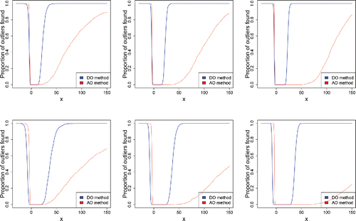
In the direction of the short left tail of the lognormal distribution we see that the adjusted outlyingness AO flags about the same percentage of outliers as the DO. But the AO is much slower in flagging outliers in the direction of the long right tail of the lognormal. This is due to the relatively high explosion bias of the scale used in the denominator of the AO for points to the right of the median. The DO flags outliers to the right of the median much faster, due to its lower explosion bias.

We have also extended the multivariate simulation of AO in Hubert and Van der Veeken (2008). Our simulation consists of m = 1000 samples in dimensions d = {2, 5, 10} and with sample sizes n = {200, 500, 1000}. The clean data were generated from the multivariate skew normal distribution (Azzalini and Dalla Valle 1996) with density $f\left(\mathbf{y}\right)=2{\varphi }_d\left(\mathbf{y}\right)\Phi \left({\alpha }^T\mathbf{y}\right)$ where Φ is the standard normal cdf, φ_p is the d-variate standard normal density, and $\alpha$ is a d-variate vector which regulates the shape. In our simulations $\alpha$ is a vector with entries equal to 10 or 4. For d = 2 we used $\alpha ={(10,4)}^T$, for d = 5 we put $\alpha ={(10,10,4,4,4)}^T$, and for d = 10 we took $\alpha ={(10,10,10,10,10,4,4,4,4,4)}^T$. 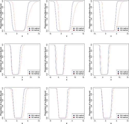To this we added 10% of contamination with a normal distribution $N(\mathbf{x},I_d/20)$ around the point $\mathbf{x}={(x,\dots ,x)}^T$, where x is on the horizontal axis of Figure 19. In d = 2 dimensions we see that AO flags the outliers a bit faster in the direction of the shortest tail, but slower in the direction of the longest tail. The latter is similar to what we saw for univariate data, due to the higher explosion bias of the scale used (implicitly) in the AO. When both the dimension d and the sample size n go up, the DO and AO methods give more similar results. This is because, in most directions, the scales s_a and s_b of the projected data get closer to each other. This is because the projections of the good data (i.e., without the outliers) tend to become more Gaussian as the dimension d and the sample size n go up, as shown by Diaconis and Freedman (1984) for random directions uniformly distributed on the unit sphere and under moment conditions on the data distribution.

Figure 19. Percentage of outliers found in multivariate skew normal samples of size n = 200 (left), n = 500 (middle), and n = 1000 (right), with 10% of outliers around $\mathbf{x}={(x,\dots ,x)}^T$, in dimensions d = 2 (top), d = 5 (middle), and d = 10 (bottom).

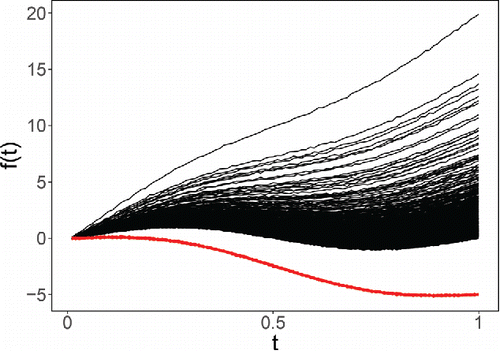
We also carried out a simulation with functional data. We have generated m = 1000 samples of n = {200, 500, 1000} functions of the form (15) $$f_i\left(t\right)=sin\left(2\pi t\right)+t{L}_i+{\epsilon }_i\left(t\right)\text{for}0⩽t⩽1,$$(15) where ln (L_i) ∼ N(0, 1) and ${\epsilon }_i\left(t\right)\sim N(0,{\left(\frac{1}{20}\right)}^2)$. That is, the base function is the sine and we add different straight lines of which the slopes are generated by a lognormal distribution. We then replace 10% of the functions by contaminated ones, which are generated from (15(15) $$f_i\left(t\right)=sin\left(2\pi t\right)+t{L}_i+{\epsilon }_i\left(t\right)\text{for}0⩽t⩽1,$$(15) ) but where L_i is taken higher or lower than what one would expect under the lognormal model. Figure 20 shows such a generated dataset of size n = 1000, with outlying functions (with negative L_i) in red.

Figure 20. n = 1000 generated functions with 10% contamination.

In the simulation we used a single slope L for the 10% of contaminated curves, and this L is shown on the horizontal axis in Figure 21. When the outlying functions lie below the regular ones (i.e., for negative L), we see that the DO and AO behave similarly. On the other hand, when the outlying functions lie above the regular ones (i.e., in the direction of the long tail), the AO is much slower to flag them than DO.

Figure 21. Percentage of outliers found in functional samples of size n = 200 (left), n = 500 (middle), and n = 1000 (right), with 10% of contaminated curves with slope L.

These simulations together suggest that the DO outperforms AO in directions where the uncontaminated data has a longer tail, while performing similarly in the other directions.

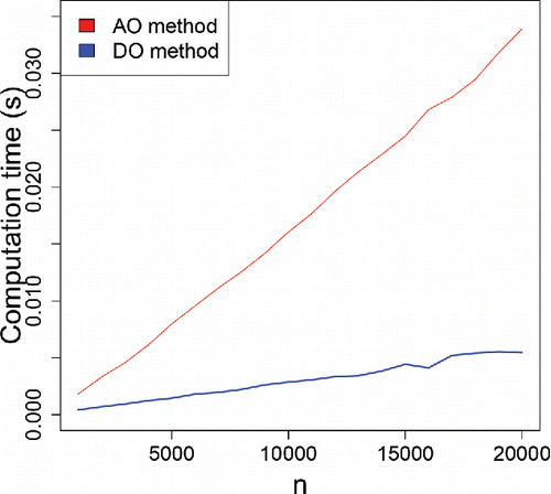
Note that the DO requires only $\mathcal{O}\left(n\right)$ computation time per direction, which is especially beneficial for functional data with a large domain. In particular, DO is much faster than AO which requires $\mathcal{O}(nlog(n\left)\right)$ operations. Figure 22 shows the average computation time (in seconds) of both measures as a function of the sample size n, for m = 1000 samples from the standard normal. The AO time is substantially above the DO time.

Figure 22. Average computation time of DO and AO as a function of sample size.

7. Conclusion

The notion of directional outlyingness (DO) is well-suited for skewed distributions. It has good robustness properties, and lends itself to the analysis of univariate, multivariate, and functional data, in which both the domain and the function values can be multivariate. Rough cutoffs for outlier detection are available. The DO is also a building block of several graphical tools like DO heatmaps, DO contours, and the functional outlier map (FOM). These proved useful when analyzing spectra, MRI images, and surveillance video. In the MRI images we added gradients to the data to reflect shape/spatial information. In video data we could also add the numerical derivative in the time direction. In our example this would make the frames six-dimensional, but the componentwise DO in (14(14) $$\text{CDO}(\mathbf{y};\mathbf{Y})=\sqrt{{\sum }_{h=1}^d\text{DO}{(y_h;Y_h)}^2},$$(14) ) would remain fast to compute.

8. Available Software

The methods described in this article are available in R (R core team 2016), in the package mrfDepth (https://CRAN.R-project.org/package=mrfDepth). An R script and the data sets for reproducing the examples in the article are available from our website http://wis.kuleuven.be/stat/robust/software.

Acknowledgments

This research has been supported by projects of Internal Funds KU Leuven. The authors are grateful for interesting discussions with Pieter Segaert.

Funding

Onderzoeksraad, KU Leuven.

Appendix

Proof of Lemma 1(i).

Let $\mu \in \mathbb{R}$ be fixed. For the function ρ_c we have that $$\begin{array}{ccc}& & t^2{\int }_{\mu }^{\infty }{\rho }_c\left(\frac{x-\mu }{t}\right)dF\left(x\right)\hfill \\ & & ={\int }_{\mu }^{\infty }\left\{{\left(\frac{x-\mu }{c}\right)}^2{\mathbb{1}}_{\left|\frac{x-\mu }{t}\right|\le c}+t^2{\mathbb{1}}_{\left|\frac{x-\mu }{t}\right|>c}\right\}dF\left(x\right)\hfill \\ & & ={\int }_0^{\infty }\left\{{\left(\frac{u}{c}\right)}^2{\mathbb{1}}_{0⩽u⩽ct}+t^2{\mathbb{1}}_{ct<u}\right\}dF(\mu +u)\hfill \end{array}$$For all u ⩾ 0 it holds that ${\left(\frac{u}{c}\right)}^2{\mathbb{1}}_{0⩽u⩽ct}+t^2{\mathbb{1}}_{ct<u}$ is nondecreasing in t, and even strictly increasing in t at large enough u. This proves (i) since f(x) > 0 in all x.

Proof of Lemma 1(ii).

Fix σ > 0. It follows from the Leibniz integral rule that $$\begin{array}{ccc}\hfill \frac{\partial }{\partial t}\left\{{\sigma }^2{\int }_t^{\infty }{\rho }_c\left(\frac{x-t}{\sigma }\right)dF\left(x\right)\right\}& =& -\sigma {\int }_t^{\infty }{\rho }_c^{\text{'}}\left(\frac{x-t}{\sigma }\right)dF\left(x\right)\hfill \end{array}$$because ρ_c(0) = 0. Note now that $$\begin{array}{ccc}\hfill {\rho }_c^{\text{'}}\left(\frac{x-t}{\sigma }\right)>0& \text{for}& t⩽x<t+\sigma c\hfill \\ \hfill {\rho }_c^{\text{'}}\left(\frac{x-t}{\sigma }\right)=0& \text{for}& x>t+\sigma c.\hfill \end{array}$$This implies that $\frac{\partial }{\partial t}\left\{{\sigma }^2{\int }_t^{\infty }{\rho }_c\left(\frac{x-t}{\sigma }\right)dF\left(x\right)\right\}<0$ for all t.

Proof of Proposition 1.

Let 0 < ϵ < 0.25 be fixed and let F_{ϵ, H} be a minimizing distribution, that is, $$\begin{array}{c}\hfill \underset{F_{\epsilon ,G}\in {\mathcal{F}}_{\epsilon ,G}}{inf}\left({\text{s}}_a\left(F_{\epsilon ,G}\right)\right)={\text{s}}_a\left(F_{\epsilon ,H}\right)\end{array}$$with F_{ϵ, G} = (1 − ϵ)F + ϵG. Inserting the contaminated distribution F_{ϵ, H} into s_a(F_{ϵ, H}) yields the scale (A.1) $$\begin{array}{ccc}& & \frac{{\text{s}}_{o,a}^2\left(F_{\epsilon ,H}\right)}{\alpha }\left\{(1-\epsilon ){\int }_{\text{med}\left(F_{\epsilon ,H}\right)}^{\infty }{\rho }_c\left(\frac{x-\text{med}\left(F_{\epsilon ,H}\right)}{{\text{s}}_{o,a}\left(F_{\epsilon ,H}\right)}\right)dF\left(x\right)\right.\hfill \\ & & \left.+\epsilon {\int }_{\text{med}\left(F_{\epsilon ,H}\right)}^{\infty }{\rho }_c\left(\frac{x-\text{med}\left(F_{\epsilon ,H}\right)}{{\text{s}}_{o,a}\left(F_{\epsilon ,H}\right)}\right)dH\left(x\right)\right\}.\hfill \end{array}$$(A.1) For simplicity, put (A.2) $$\begin{array}{ccc}\hfill W_1\left(F_{\epsilon ,H}\right)& =& {\int }_{\text{med}\left(F_{\epsilon ,H}\right)}^{\infty }{\rho }_c\left(\frac{x-\text{med}\left(F_{\epsilon ,H}\right)}{{\text{s}}_{o,a}\left(F_{\epsilon ,H}\right)}\right)dF\left(x\right)\hfill \\ \hfill W_2\left(F_{\epsilon ,H}\right)& =& {\int }_{\text{med}\left(F_{\epsilon ,H}\right)}^{\infty }{\rho }_c\left(\frac{x-\text{med}\left(F_{\epsilon ,H}\right)}{{\text{s}}_{o,a}\left(F_{\epsilon ,H}\right)}\right)dH\left(x\right).\hfill \end{array}$$(A.2) We then have the contaminated scale (A.3) $$\frac{{\text{s}}_{o,a}^2\left(F_{\epsilon ,H}\right)}{\alpha }\{(1-\epsilon )W_1\left(F_{\epsilon ,H}\right)+\epsilon W_2\left(F_{\epsilon ,H}\right)\}.$$(A.3) Denote by Q_{2, ϵ} = F^{− 1}_{ϵ, H}(0.5) and Q_{3, ϵ} = F^{− 1}_{ϵ, H}(0.75) the median and the third quartile of the contaminated distribution.

For the distribution H it has to hold that H(Q_{3, ϵ}) = 1 and ${lim}_{x\to Q_{2,\epsilon }^{-}}H\left(x\right)=0$. This can be seen as follows. Suppose H(∞) − H(Q_{3, ϵ}) = p ∈ (0, 1]. Then consider $F_{\epsilon ,H^{*}}$ where $$\begin{array}{c}\hfill H^{*}\left(x\right)=\left\{\begin{array}{cc}\hfill H\left(x\right)+p\Delta \left(Q_{2,\epsilon }\right)& \hfill \text{for}x\in (-\infty ,Q_{3,\epsilon }]\\ \hfill 1& \hfill \text{else}\end{array}\right.\end{array}$$and denote by Q*_{2, ϵ} and Q*_{3, ϵ} the median and third quartile of $F_{\epsilon ,H^{*}}$. Note that Q_{2, ϵ} = Q*_{2, ϵ} and Q_{3, ϵ} > Q*_{3, ϵ}. Therefore, we have ${\text{s}}_{o,a}\left(F_{\epsilon ,H}\right)>{\text{s}}_{o,a}\left(F_{\epsilon ,H^{*}}\right)$. It then follows from Lemma 1(i) that ${\text{s}}_{o,a}{\left(F_{\epsilon ,H}\right)}^2(1-\epsilon )W_1\left(F_{\epsilon ,H}\right)>{\text{s}}_{o,a}{\left(F_{\epsilon ,H^{*}}\right)}^2(1-\epsilon )W_1\left(F_{\epsilon ,H^{*}}\right)$ and $W_2\left(F_{\epsilon ,H}\right)>W_2\left(F_{\epsilon ,H^{*}}\right)=0$. Therefore, ${\text{s}}_{o,a}{\left(F_{\epsilon ,H}\right)}^2\epsilon W_2\left(F_{\epsilon ,H}\right)>{\text{s}}_{o,a}{\left(F_{\epsilon ,H^{*}}\right)}^2\epsilon W_2\left(F_{\epsilon ,H^{*}}\right)$. It now follows that ${\text{s}}_a\left(F_{\epsilon ,H^{*}}\right)<{\text{s}}_a\left(F_{\epsilon ,H}\right)$, which is a contradiction since H minimizes s_a. Therefore, H(∞) − H(Q_{3, ϵ}) = 0. A similar argument can be made to show that ${lim}_{x\to Q_{2,\epsilon }^{-}}H\left(x\right)=0$. It follows that H(Q_{3, ϵ}) = 1 and H(x) = 0 for all x < Q_{2, ϵ}, so all the mass of H is inside [Q_{2, ϵ} , Q_{3, ϵ}].

We can now argue that H must have all its mass in Q_{2, ϵ}. Note that if H(Q_{3, ϵ}) = 1 and ${lim}_{x\to Q_{2,\epsilon }^{-}}H\left(x\right)=0$ we have $Q_{2,\epsilon }=F^{-1}\left(\frac{1}{2(1-\epsilon )}\right)$ and $Q_{3,\epsilon }\in [F^{-1}\left(\frac{3-4\epsilon }{4(1-\epsilon )}\right),F^{-1}\left(\frac{3}{4(1-\epsilon )}\right)]$, depending on ${lim}_{x\to Q_{3,\epsilon }^{-}}H\left(x\right)$. Given that Q_{2, ϵ} is fixed, we can minimize W₁(F_{ϵ, H}) by minimizing Q_{3, ϵ}. Now Q_{3, ϵ} is minimal for $H=\Delta \left(F^{-1}\left(\frac{1}{2(1-\epsilon )}\right)\right)$ as this yields $Q_{3,\epsilon }=F^{-1}\left(\frac{3-4\epsilon }{4(1-\epsilon )}\right)$. Note that this choice of H to minimize Q_{3, ϵ} is not unique as any H which makes ${lim}_{x\to Q_{3,\epsilon }^{-}}H\left(x\right)=1$ does the job. Note finally that W₂(F_{ϵ, H}) is also minimal for $H=\Delta \left(F^{-1}\left(\frac{1}{2(1-\epsilon )}\right)\right)$ as ρ_c(t) is nondecreasing in |t|, and this choice of H yields W₂(F_{ϵ, H}) = 0.

We now know that $H=\Delta \left(F^{-1}\left(\frac{1}{2(1-\epsilon )}\right)\right)$ minimizes s_a(F_{ϵ, H}). Furthermore, we have $Q_{2,\epsilon }=F^{-1}\left(\frac{1}{2(1-\epsilon )}\right)=B^{+}(\epsilon ,\text{med},F)$ and $Q_{3,\epsilon }=F^{-1}\left(\frac{3-4\epsilon }{4(1-\epsilon )}\right)$. Therefore, the implosion bias of s_a is $$\begin{array}{ccc}& & B^{-}{(\epsilon ,{\text{s}}_a,F)}^2=\frac{B^{-}{(\epsilon ,{\text{s}}_{o,a},F)}^2}{\alpha }\hfill \\ & & \times \left\{(1-\epsilon ){\int }_{B^{+}(\epsilon ,\text{med},F)}^{\infty }{\rho }_c\left(\frac{x-B^{+}(\epsilon ,\text{med},F)}{B^{-}(\epsilon ,{\text{s}}_{o,a},F)}\right)dF\left(x\right)\right\},\hfill \end{array}$$where $$\begin{array}{ccc}\hfill B^{+}(\epsilon ,\text{med},F)& =& F^{-1}\left(\frac{1}{2(1-\epsilon )}\right)\hfill \\ \hfill B^{-}(\epsilon ,{\text{s}}_{o,a},F)& =& \left(F^{-1}\left(\frac{3-4\epsilon }{4(1-\epsilon )}\right)-F^{-1}\left(\frac{1}{2(1-\epsilon )}\right)\right)\hfill \\ & & /{\Phi }^{-1}(0.75).\hfill \end{array}$$

Proof of Proposition 2.

Let 0 < ϵ < 0.25 be fixed and let F_{ϵ, H} be a maximizing distribution, that is, $$\begin{array}{c}\hfill \underset{F_{\epsilon ,G}\in {\mathcal{F}}_{\epsilon ,G}}{sup}\left({\text{s}}_a\left(F_{\epsilon ,G}\right)\right)={\text{s}}_a\left(F_{\epsilon ,H}\right)\end{array}$$with F_{ϵ, G} = (1 − ϵ)F + ϵG. Inserting the contaminated distribution F_{ϵ, H} into s_a(F_{ϵ, H}) yields the scale (A.1(A.1) $$\begin{array}{ccc}& & \frac{{\text{s}}_{o,a}^2\left(F_{\epsilon ,H}\right)}{\alpha }\left\{(1-\epsilon ){\int }_{\text{med}\left(F_{\epsilon ,H}\right)}^{\infty }{\rho }_c\left(\frac{x-\text{med}\left(F_{\epsilon ,H}\right)}{{\text{s}}_{o,a}\left(F_{\epsilon ,H}\right)}\right)dF\left(x\right)\right.\hfill \\ & & \left.+\epsilon {\int }_{\text{med}\left(F_{\epsilon ,H}\right)}^{\infty }{\rho }_c\left(\frac{x-\text{med}\left(F_{\epsilon ,H}\right)}{{\text{s}}_{o,a}\left(F_{\epsilon ,H}\right)}\right)dH\left(x\right)\right\}.\hfill \end{array}$$(A.1) ), which can be rewritten as in (A.2(A.2) $$\begin{array}{ccc}\hfill W_1\left(F_{\epsilon ,H}\right)& =& {\int }_{\text{med}\left(F_{\epsilon ,H}\right)}^{\infty }{\rho }_c\left(\frac{x-\text{med}\left(F_{\epsilon ,H}\right)}{{\text{s}}_{o,a}\left(F_{\epsilon ,H}\right)}\right)dF\left(x\right)\hfill \\ \hfill W_2\left(F_{\epsilon ,H}\right)& =& {\int }_{\text{med}\left(F_{\epsilon ,H}\right)}^{\infty }{\rho }_c\left(\frac{x-\text{med}\left(F_{\epsilon ,H}\right)}{{\text{s}}_{o,a}\left(F_{\epsilon ,H}\right)}\right)dH\left(x\right).\hfill \end{array}$$(A.2) ) and (A.3(A.3) $$\frac{{\text{s}}_{o,a}^2\left(F_{\epsilon ,H}\right)}{\alpha }\{(1-\epsilon )W_1\left(F_{\epsilon ,H}\right)+\epsilon W_2\left(F_{\epsilon ,H}\right)\}.$$(A.3) ).

For the distribution H it has to hold that H(Q_{3, ϵ}) = lim_{x → Q⁻2, ϵ}H(x). This can be seen as follows. Suppose H(Q_{3, ϵ}) − lim_{x → Q⁻2, ϵ}H(x) = p ∈ (0, 1]. Now put $e=B^{+}(\epsilon ,\text{med},F)+c{B}^{+}(\epsilon ,{\text{s}}_{o,a},F)$ and consider the distribution $F_{\epsilon ,H^{*}}$ where $$\begin{array}{c}\hfill H^{*}\left(x\right)=\left\{\begin{array}{cc}\hfill H\left(x\right)& \hfill \text{for}x\in (-\infty ,Q_{2,\epsilon })\\ \hfill \underset{x\to Q_{2,\epsilon }^{-}}{lim}H\left(x\right)& \hfill \text{for}x\in [Q_{2,\epsilon },Q_{3,\epsilon }]\\ \hfill H\left(x\right)-p+p\Delta \left(e\right)& \hfill \text{for}x\in (Q_{3,e},\infty )\end{array}\right.\end{array}$$and denote by Q*_{2, ϵ} and Q*_{3, ϵ} the median and third quartile of $F_{\epsilon ,H^{*}}$. Note that Q_{2, ϵ} = Q*_{2, ϵ} and Q_{3, ϵ} < Q*_{3, ϵ}. Therefore ${\text{s}}_{o,a}\left(F_{\epsilon ,H}\right)<{\text{s}}_{o,a}\left(F_{\epsilon ,H^{*}}\right)$ and thus ${\text{s}}_{o,a}{\left(F_{\epsilon ,H}\right)}^2(1-\epsilon )W_1\left(F_{\epsilon ,H}\right)<{\text{s}}_{o,a}{\left(F_{\epsilon ,H^{*}}\right)}^2(1-\epsilon )W_1\left(F_{\epsilon ,H^{*}}\right)$ because of Lemma 1(i). Furthermore, $W_2\left(F_{\epsilon ,H}\right)<W_2\left(F_{\epsilon ,H^{*}}\right)$ because ρ_c(t) is nondecreasing in |t|, thus ${\text{s}}_{o,a}{\left(F_{\epsilon ,H}\right)}^2\epsilon W_2\left(F_{\epsilon ,H}\right)<{\text{s}}_{o,a}{\left(F_{\epsilon ,H^{*}}\right)}^2\epsilon W_2\left(F_{\epsilon ,H^{*}}\right)$. It now follows that ${\text{s}}_a\left(F_{\epsilon ,H^{*}}\right)>{\text{s}}_a\left(F_{\epsilon ,H}\right)$, which is a contradiction since H maximizes s_a. Therefore H(Q_{3, ϵ}) = lim_{x → Q⁻2, ϵ}H(x), so H has no mass inside [Q_{2, ϵ} , Q_{3, ϵ}].

Without loss of generality we can thus assume that H is of the form H = dΔ(e₁) + (1 − d)Δ(e₂) with $e_1=B^{-}(\epsilon ,\text{med},F)-c{B}^{+}(\epsilon ,{\text{s}}_{o,a},F)$ and $e_2=B^{+}(\epsilon ,\text{med},F)+c{B}^{+}(\epsilon ,{\text{s}}_{o,a},F)$ where d ∈ [0, 1]. This choice of e₁ and e₂ is not unique but it maximizes s_a(F_{ϵ, H}) because ρ_c(t) is nondecreasing in |t|. Inserting the distribution F_d ≔ F_{ϵ, H} yields (A.4) $$\begin{array}{c}\hfill {\text{s}}_a^2\left(F_d\right)=\frac{{\text{s}}_{o,a}^2\left(F_d\right)}{\alpha }\left\{(1-\epsilon ){\int }_{Q_{2,d}}^{\infty }{\rho }_c\left(\frac{x-Q_{2,d}}{{\text{s}}_{o,a}\left(F_d\right)}\right)dF\left(x\right)+\epsilon (1-d)\right\},\end{array}$$(A.4) where $Q_{2,d}=F^{-1}\left(\frac{1-2d\epsilon }{2(1-\epsilon )}\right)$, $Q_{3,d}=F^{-1}\left(\frac{3-4d\epsilon }{4(1-\epsilon )}\right)$, and s_{o, a}(F_d) = (Q_{3, d} − Q_{2, d})/Φ^{− 1}(0.75). Note that this expression depends on d but no longer on e₁ and e₂. We will show that this expression is maximized for d = 0.

First we show that s_{o, a}(F_d) is maximized for d = 0. Let (A.5) $$g\left(d\right):={\text{s}}_{o,a}\left(F_d\right)=(Q_{3,d}-Q_{2,d})/{\Phi }^{-1}(0.75)$$(A.5) for any d ∈ [0, 1]. Note that $\xi =\frac{3-4\epsilon d}{4(1-\epsilon )}-\frac{2-4\epsilon d}{4(1-\epsilon )}=\frac{1}{4(1-\epsilon )}$ does not depend on d. Therefore, we can write g(d) = (F^{− 1}(v + ξ) − F^{− 1}(v))/Φ^{− 1}(0.75) where $v=\frac{2-4\epsilon d}{4(1-\epsilon )}$ is a strictly decreasing function of d. Note that we can write $g\left(d\right)={\left({\Phi }^{-1}(0.75)\right)}^{-1}{\int }_v^{v+\xi }\frac{du}{f\left(F^{-1}\left(u\right)\right)}$. The density f is symmetric about some m, and by affine equivariance we can assume m = 0 w.l.o.g. Since f is unimodal with f(x) > 0 for all x, the function $u\to \frac{1}{f\left(F^{-1}\left(u\right)\right)}$ is strictly decreasing up to its minimum (corresponding to the mode of f) and then strictly increasing. Therefore, g(d) is maximal for v as large as possible, that is, for d = 0. In that case, we have $v=Q_{2,o}=\frac{2}{4(1-\epsilon )}>0.5$.

Next, we maximize (A.6) $$h(\sigma ,d):=\frac{{\sigma }^2}{\alpha }\left\{(1-\epsilon ){\int }_{Q_{2,d}}^{\infty }{\rho }_c\left(\frac{x-Q_{2,d}}{\sigma }\right)dF\left(x\right)+\epsilon (1-d)\right\}$$(A.6) for any fixed σ > 0. This is equivalent to maximizing (A.7) $${\int }_q^{\infty }{\rho }_c\left(\frac{x-q}{\sigma }\right)dF\left(x\right)+\frac{\epsilon }{1-\epsilon }(1-d),$$(A.7) where q is such that $F\left(q\right)\in [\frac{1-2\epsilon }{2(1-\epsilon )},\frac{1}{2(1-\epsilon )}]=\frac{1}{2}\pm \frac{\epsilon }{1-\epsilon }$. Note that $\frac{\epsilon }{1-\epsilon }(1-d)=F\left(q\right)+\frac{1-2\epsilon }{2(1-\epsilon )}$, where the second term doesn’t depend on q. Maximizing (A.7(A.7) $${\int }_q^{\infty }{\rho }_c\left(\frac{x-q}{\sigma }\right)dF\left(x\right)+\frac{\epsilon }{1-\epsilon }(1-d),$$(A.7) ) with respect to q is therefore equivalent to maximizing ${\int }_q^{q+c\sigma }{\left(\frac{x-q}{c\sigma }\right)}^{2}dF\left(x\right)-{\int }_q^{q+c\sigma }dF\left(x\right)$. Note that this is equal to ${\int }_0^{c\sigma }{\left(\frac{x}{c\sigma }\right)}^{2}dF(q+x)-{\int }_0^{c\sigma }dF(q+x)={\int }_0^{c\sigma }\frac{x^2-{\sigma }^2{c}^2}{{\sigma }^2{c}^2}f(q+x)d\left(x\right)$. For all x in [0, cσ] it holds that $\frac{x^2-{\sigma }^2{c}^2}{{\sigma }^2{c}^2}\le 0$, hence the latter integral is maximized by minimizing f(q + x) for all x ∈ [0, cσ]. For this q must take on its highest possible value $q=F^{-1}(\frac{1}{2}+\frac{\epsilon }{1-\epsilon })$, because we then have f(q + x) ⩽ f(q₂ + x) for all x in [0, cσ] and all q₂ in $[F^{-1}(\frac{1}{2}-\frac{\epsilon }{1-\epsilon }),F^{-1}(\frac{1}{2}+\frac{\epsilon }{1-\epsilon })]$. Therefore, (A.6(A.6) $$h(\sigma ,d):=\frac{{\sigma }^2}{\alpha }\left\{(1-\epsilon ){\int }_{Q_{2,d}}^{\infty }{\rho }_c\left(\frac{x-Q_{2,d}}{\sigma }\right)dF\left(x\right)+\epsilon (1-d)\right\}$$(A.6) ) is maximized for d = 0.

We now know that (A.5(A.5) $$g\left(d\right):={\text{s}}_{o,a}\left(F_d\right)=(Q_{3,d}-Q_{2,d})/{\Phi }^{-1}(0.75)$$(A.5) ) and (A.6(A.6) $$h(\sigma ,d):=\frac{{\sigma }^2}{\alpha }\left\{(1-\epsilon ){\int }_{Q_{2,d}}^{\infty }{\rho }_c\left(\frac{x-Q_{2,d}}{\sigma }\right)dF\left(x\right)+\epsilon (1-d)\right\}$$(A.6) ) satisfy max _dg(d) = g(0) and max _dh(σ, d) = h(σ, 0) for all σ > 0. By Lemma 1(i), h(σ, 0) is increasing in σ. Combining these results yields $$\begin{array}{ccc}\hfill \underset{d}{max}{\text{s}}_a^2\left(F_d\right)& =& \underset{d}{max}h(g\left(d\right),d)\hfill \\ & ⩽& \underset{d_1}{max}\underset{d_2}{max}h(g\left(d_1\right),d_2)\hfill \\ & =& \underset{d_1}{max}h(g\left(d_1\right),0)\hfill \\ & =& h\left(g\right(0),0),\hfill \end{array}$$so s²_a(F_d) is maximized for d = 0. Therefore, s²_a(F_{ϵ, H}) is maximized for H = Δ(e₂), hence $Q_{2,\epsilon }=F^{-1}\left(\frac{1}{2(1-\epsilon )}\right)=B^{+}(\epsilon ,\text{med},F)$ and $Q_{3,\epsilon }=F^{-1}\left(\frac{3}{4(1-\epsilon )}\right)$. The explosion bias is thus $$\begin{array}{ccc}& & B^{+}{(\epsilon ,{\text{s}}_a,F)}^2\hfill \\ & & =\frac{{\text{s}}_{o,a}^2}{\alpha }\left\{(1-\epsilon ){\int }_{B^{+}(\epsilon ,\text{med},F)}^{\infty }{\rho }_c\left(\frac{x-B^{+}(\epsilon ,\text{med},F)}{{\text{s}}_{o,a}}\right)dF\left(x\right)+\epsilon \right\},\hfill \end{array}$$where $$\begin{array}{ccc}\hfill {\text{s}}_{o,a}& =& \left\{F^{-1}\left(\frac{3}{4(1-\epsilon )}\right)-F^{-1}\left(\frac{1}{2(1-\epsilon )}\right)\right\}/{\Phi }^{-1}(0.75).\hfill \end{array}$$

Proof of Proposition 3.

Plugging the contaminated distribution F_{ϵ, z} = (1 − ϵ)F + ϵΔz into the functional form (4(4) $$\begin{array}{ccc}\hfill {\text{s}}_a^2\left(F\right)& =& \frac{{\text{s}}_{o,a}^2\left(F\right)}{\alpha }{\int }_{\mathrm{med}\left(F\right)}^{\infty }{\rho }_c\left(\frac{x-\text{med}\left(F\right)}{{\text{s}}_{o,a}\left(F\right)}\right)dF\left(x\right)\hfill \\ \hfill {\text{s}}_b^2\left(F\right)& =& \frac{{\text{s}}_{o,b}^2\left(F\right)}{\alpha }{\int }_{-\infty }^{\mathrm{med}\left(F\right)}{\rho }_c\left(\frac{\text{med}\left(F\right)-x}{{\text{s}}_{o,b}\left(F\right)}\right)dF\left(x\right),\hfill \end{array}$$(4) ) of s_a yields $$\begin{array}{c}\hfill {\text{s}}_a^2\left(F_{\epsilon ,z}\right)=\frac{{\text{s}}_{o,a}^2\left(F_{\epsilon ,z}\right)}{\alpha }{\int }_{\text{med}\left(F_{\epsilon ,z}\right)}^{\infty }{\rho }_c\left(\frac{x-\text{med}\left(F_{\epsilon ,z}\right)}{{\text{s}}_{o,a}\left(F_{\epsilon ,z}\right)}\right)d{F}_{\epsilon ,z}\left(x\right).\end{array}$$We take the derivative with respect to ϵ and evaluate it in ϵ = 0. Note that ρ_c(t) is not differentiable at t = c and t = −c, but as these two points form a set of measure zero this does not affect the integral containing ρ′_c(t). We also use that ρ_c(0) = 0 and IF(z, s²_a, F) = 2s_a(F)IF(z, s_a, F) yielding the desired expression. For F = Φ we have $\text{IF}(z,{\text{s}}_{o,a},\Phi )=({\mathbb{1}}_{\left\{\right[0,\infty \left)\right\}}\left(z\right)\mathrm{sign}(z-{\Phi }^{-1}\left(\frac{3}{4}\right))+\text{IF}(z,\text{med},\Phi )\{\varphi \left(0\right)-2\varphi \left({\Phi }^{-1}\left(\frac{3}{4}\right)\right)\})/\left(2\varphi \left({\Phi }^{-1}\left(\frac{3}{4}\right)\right)\right)$.

Proof of Proposition 4.

We show the proof for $x>\text{med}\left(F\right)$, the other case being analogous. Plugging the contaminated distribution F_{ϵ, z} = (1 − ϵ)F + ϵΔz into $\text{DO}(x,F)=(x-\text{med}\left(F\right))/{\text{s}}_a\left(F\right)$ yields $$\begin{array}{ccc}\hfill \text{IF}(z,\text{DO}(x),F)& =& \frac{\partial }{\partial \epsilon }\left(\text{DO}(x,F_{\epsilon ,z})\right){|}_{\epsilon =0}=\frac{1}{{\text{s}}_a^2\left(F_{\epsilon ,z}\right)}(-\frac{\partial }{\partial \epsilon }(\text{med}\left(F_{\epsilon ,z}\right))\hfill \\ & & \times {\text{s}}_a\left(F_{\epsilon ,z}\right)-\frac{\partial }{\partial \epsilon }\left({\text{s}}_a\left(F_{\epsilon ,z}\right)\right)(x-\text{med}\left(F_{\epsilon ,z}\right)){\left)\right|}_{\epsilon =0}\hfill \\ & =& \frac{1}{{\text{s}}_a^2\left(F\right)}(-\text{IF}(z,\text{med},F){\text{s}}_a\left(F\right)\hfill \\ & & -\text{IF}(z,{\text{s}}_a,F)(x-\text{med}\left(F\right))).\hfill \end{array}$$

References

- Arribas-Gil, A., and Romo, J. (2014), “Shape Outlier Detection and Visualization for Functional Data: The Outliergram,” Biostatistics, 15, 603–619.
- Azzalini, A., and Dalla Valle, A. (1996), “The Multivariate Skew-Normal Distribution,” Biometrika, 83, 715–726.
- Berrendero, J., Justel, A., and Svarc, M. (2011), “‘Principal Components for Multivariate Functional Data,” Computational Statistics & Data Analysis, 55, 2619–2634.
- Brys, G., Hubert, M., and Rousseeuw, P. J. (2005), “A Robustification of Independent Component Analysis,” Journal of Chemometrics, 19, 364–375.
- Brys, G., Hubert, M., and Struyf, A. (2004), “A Robust Measure of Skewness,” Journal of Computational and Graphical Statistics, 13, 996–1017.
- Diaconis, P., and Freedman, D. (1984), “Asymptotics of Graphical Projection Pursuit,” The Annals of Statistics, 12, 793–815.
- Donoho, D. (1982), Breakdown Properties of Multivariate Location Estimators, Ph.D. dissertation, Department of Statistics, Harvard University.
- Febrero-Bande, M., Galeano, P., and González-Manteiga, W. (2008), “Outlier Detection in Functional Data by Depth Measures, With Application to Identify Abnormal NOx Levels,” Environmetrics, 19, 331–345.
- Ferraty, F., and Vieu, P. (2006), Nonparametric Functional Data Analysis: Theory and Practice, New York, NY: Springer.
- Hampel, F., Ronchetti, E., Rousseeuw, P., and Stahel, W. (1986), Robust Statistics: The Approach Based on Influence Functions, New York: Wiley.
- Hand, D., Lunn, A., McConway, A., and Ostrowski, E. (1994), A Handbook of Small Data Sets, London, UK: Chapman and Hall.
- Hubert, M., Rousseeuw, P. J., and Segaert, P. (2015), “Multivariate Functional Outlier Detection” (with discussion), Statistical Methods & Applications, 24, 177–246.
- Hubert, M., and Van der Veeken, S. (2008), “Outlier Detection for Skewed Data,” Journal of Chemometrics, 22, 235–246.
- Hyndman, R., and Shang, H. (2010), “Rainbow Plots, Bagplots, and Boxplots for Functional Data,” Journal of Computational and Graphical Statistics, 19, 29–45.
- Lemberge, P., De Raedt, I., Janssens, K., Wei, F., and Van Espen, P. (2000), “Quantitative Z-Analysis of 16th–17th Century Archaeological Glass Vessels Using PLS Regression of EPXMA and μ-XRF Data,” Journal of Chemometrics, 14, 751–763.
- Li, L., Huang, W., Gu, I. Y.-H., and Tian, Q. (2004), “Statistical Modeling of Complex Backgrounds for Foreground Object Detection,” IEEE Transactions on Image Processing, 13, 1459–1472.
- Marcus, D., Wang, T., Parker, J., Csernansky, J., Morris, J., and Buckner, R. (2007), “Open Access Series of Imaging Studies (OASIS): Cross-Sectional MRI Data in Young, Middle Aged, Nondemented, and Demented Older Adults,” Journal of Cognitive Neuroscience, 19, 1498–1507.
- Martin, R., and Zamar, R. (1993), “Bias Robust Estimation of Scale,” The Annals of Statistics, 21, 991–1017.
- Pigoli, D., and Sangalli, L. (2012), “Wavelets in Functional Data Analysis: Estimation of Multidimensional Curves and Their Derivatives,” Computational Statistics & Data Analysis, 56, 1482–1498.
- R Core Team (2016), “R: A Language and Environment for Statistical Computing,” R Foundation for Statistical Computing, Vienna, Austria. Available at: https://www.R-project.org/
- Ramsay, J., and Silverman, B. (2005), Functional Data Analysis (2nd ed.), New York: Springer.
- Rousseeuw, P., and Croux, C. (1994), “The Bias of k-Step M-Estimators,” Statistics & Probability Letters, 20, 411–420.
- Stahel, W. (1981), Robuste Schätzungen: Infinitesimale Optimalität und Schätzungen von Kovarianzmatrizen, Ph.D. dissertation. Switzerland: ETHZürich.
- Sun, Y., and Genton, M. (2011), “Functional Boxplots,” Journal of Computational and Graphical Statistics, 20, 316–334.