Dynamically Updated Spatially Varying Parameterizations of Hierarchical Bayesian Models for Spatial Data

ABSTRACT

Fitting hierarchical Bayesian models to spatially correlated datasets using Markov chain Monte Carlo (MCMC) techniques is computationally expensive. Complicated covariance structures of the underlying spatial processes, together with high-dimensional parameter space, mean that the number of calculations required grows cubically with the number of spatial locations at each MCMC iteration. This necessitates the need for efficient model parameterizations that hasten the convergence and improve the mixing of the associated algorithms. We consider partially centred parameterizations (PCPs) which lie on a continuum between what are known as the centered (CP) and noncentered parameterizations (NCP). By introducing a weight matrix we remove the conditional posterior correlation between the fixed and the random effects, and hence construct a PCP which achieves immediate convergence for a three-stage model, based on multiple Gaussian processes with known covariance parameters. When the covariance parameters are unknown we dynamically update the parameterization within the sampler. The PCP outperforms both the CP and the NCP and leads to a fully automated algorithm which has been demonstrated in two simulation examples. The effectiveness of the spatially varying PCP is illustrated with a practical dataset of nitrogen dioxide concentration levels. Supplemental materials consisting of appendices, datasets, and computer code to reproduce the results are available online.

KEYWORDS:

• Gibbs sampling
• Parameterization
• Rate of convergence
• Spatially varying coefficient model

1. Introduction

There is a growing interest among researchers in spatially varying coefficient (SVC) models (Hamm et al. 2015; Wheeler et al. 2014; Finley, Banerjee, and MacFarlane 2011; Berrocal, Gelfand, and Holland 2010; Gelfand et al. 2003). Conditional independencies determined by the hierarchical structure of the model facilitate the construction of Gibbs sampling type algorithms for model fitting (Gelfand and Smith 1990). A requirement of these algorithms is the repeated inversion of dense n × n covariance matrices, an operation of order O(n³) in computational complexity, for n spatial locations (Cressie and Johannesson 2008). This, coupled with high posterior correlation between model parameters and weakly identified covariance parameters, means that fitting these models is challenging and computationally expensive. To mitigate the computational expense practitioners require efficient model fitting strategies that produce Markov chains which converge quickly to the posterior distribution and exhibit low autocorrelation between successive iterates.

Parameterization of a hierarchical model is known to affect the performance of the Markov chain Monte Carlo (MCMC) method used for inference. For normal linear hierarchical models (NLHMs) the centred parameterization (CP) yields an efficient Gibbs sampler when the variance of the data model is low relative to that of the random effects, and the noncentered parameterization (NCP) yields an efficient Gibbs sampler when the variance of the data model is relatively high (Papaspiliopoulos, Roberts, and Sköld 2003, Gelfand, Sahu, and Carlin 1995). Where the latent variables are realizations of a spatial process with an exponential correlation function, Bass and Sahu (2017) showed that increasing the strength of correlation improves the efficiency of the CP but degrades that of the NCP. Hence the sampling efficiency of the CP and the NCP is dependent upon the typically unknown variance and spatial correlation parameters and will therefore differ across different datasets. Consequently, deciding which parameterization to employ can be problematic.

With the aim of developing a robust parameterization for NLHMs, Papaspiliopoulos, Roberts, and Sköld (2003) considered the CP and the NCP as extremes of a family of partially centred parameterizations (PCPs). They find the optimal PCP which results in a Gibbs sampler that produces independent samples from the posterior distributions of the mean parameters, but again this is conditioned on the covariance parameters. The question we look to answer in this article is can we create a parameterization for spatial models that is robust to the data and does not require a priori knowledge of the model parameters, and hence can be routinely implemented?

To address this question, we write a general SVC model as a three-stage NLHM. The PCP is constructed by introducing a weight matrix that allows us to eliminate the conditional posterior correlation between the global and random effects. This in turn implies immediate convergence of the associated Gibbs sampler for known variance and correlation parameters, which collectively we will call the covariance parameters. When these parameters are unknown we propose dynamically updating the weight matrix, which leads to a parameterization that is both spatially varying and dynamically updated within the Gibbs sampler. As it is necessary to invert an n × n matrix to compute the weight matrix, implementing the PCP results in an algorithm with longer run times than those associated with the CP and NCP. Consequently, we recommend this method for modest sized spatial datasets of hundreds, but not thousands, of observations.

For an exponential correlation function, we demonstrate how the weights of partial centering depend on the covariance parameters and the sampling locations, and hence vary over the spatial domain. We show that weights are higher when the data variance is relatively low and when the spatial correlation is high. Also, higher weights are given to more densely clustered sampling locations and where the covariate values are higher. To judge sampling efficiency of the PCP we use well known convergence diagnostics. The performance of the PCP is shown to be robust to changes in the covariance parameters of the data generating mechanism. Moreover, the PCP converges more quickly and produces posterior samples with lower autocorrelation than either the CP or the NCP. Note that Bass and Sahu (2017) did not consider the PCP at all.

A related approach is the interweaving algorithm proposed by Yu and Meng (2011). The algorithm results in a Gibbs sampler that is more efficient than the worst of the CP and NCP. However, the interweaving algorithm does not guarantee immediate convergence for known covariance parameters, whereas the PCP does, see Section A.3. Another approach is to marginalize over the random effects, thus reducing the dimension of the posterior distribution. This method can be employed when the error structures of the data and the random effects are both assumed to be Gaussian. Marginalized likelihoods are used by Gelfand et al. (2003) for fitting SVC regression models. However, marginalization results in a loss of conditional conjugacy of the variance parameters and means that they have to be updated by using Metropolis-type steps, which require difficult and time consuming tuning. The scheme proposed here is fully automated.

The rest of this article is laid out as follows. Section 2 gives details of the general spatial model and the construction and properties of its PCP. Section 3 illustrates how the weights of partial centering are influenced by the model parameters and the sampling locations. Section 4 demonstrates the sampling efficiency of the PCP by applying it to simulated spatial datasets and compares its performance to the CP and the NCP. Section 5 applies the different model parameterizations to a real air pollution dataset on annual mean concentration levels of NO₂ observed in Greater London in 2011. Section 6 contains some concluding remarks.

MCMC samplers are coded in the C programming language and the output is analyzed in R (R Core Team 2016).

2. Partial Centering of Space-Varying Coefficient Models

2.1. Model Specification

For data observed at a set of locations ${\mathbf{s}}_1,\dots ,{\mathbf{s}}_n$ we consider the normal linear model with spatially varying regression coefficients (Gelfand et al. 2003): (1) $$\begin{array}{ccc}\hfill Y\left({\mathbf{s}}_i\right)& =& {\theta }_0+{\beta }_0\left({\mathbf{s}}_i\right)+\sum _{k=1}^{p-1}\{{\theta }_k+{\beta }_k\left({\mathbf{s}}_i\right)\}{x}_k\left({\mathbf{s}}_i\right)+ϵ\left({\mathbf{s}}_i\right),\hfill \\ & & i=1,\dots ,n.\hfill \end{array}$$(1) We model errors $ϵ\left({\mathbf{s}}_i\right)$ as independent and normally distributed with mean zero and variance σ²_ε. Spatially indexed observations $\mathbf{Y}={\{Y\left({\mathbf{s}}_1\right),\dots ,Y\left({\mathbf{s}}_n\right)\}}^{\mathrm{T}}$ are conditionally independent and normally distributed as $$Y\left({\mathbf{s}}_i\right)\sim N\left({\mathbf{x}}^{\mathrm{T}}\left({\mathbf{s}}_i\right)\{\mathbf{\theta }+\mathbf{\beta }\left({\mathbf{s}}_i\right)\},{\sigma }_{ϵ}^2\right),$$where $\mathbf{x}\left({\mathbf{s}}_i\right)={\{1,x_1\left({\mathbf{s}}_i\right),\dots ,x_{p-1}\left({\mathbf{s}}_i\right)\}}^{\mathrm{T}}$ is a vector containing covariate information for site ${\mathbf{s}}_i$ and $\mathbf{\theta }={({\theta }_0,\dots ,{\theta }_{p-1})}^{\mathrm{T}}$ is a vector of global regression coefficients. The kth element of $\mathbf{\theta }$ is locally perturbed by a realization of a zero mean Gaussian process, denoted ${\beta }_k\left({\mathbf{s}}_i\right)$, which are collected into a vector $\mathbf{\beta }\left({\mathbf{s}}_i\right)={\{{\beta }_0\left({\mathbf{s}}_i\right),\dots ,{\beta }_{p-1}\left({\mathbf{s}}_i\right)\}}^{\mathrm{T}}$. The n realizations of the Gaussian process associated with the kth covariate are given by ${\mathbf{\beta }}_k={\{{\beta }_k\left({\mathbf{s}}_1\right),\dots ,{\beta }_k\left({\mathbf{s}}_n\right)\}}^{\mathrm{T}}\sim N(0,{\mathbf{\Sigma }}_k),k=0,\dots ,p-1,$ where ${\mathbf{\Sigma }}_k={\sigma }_k^2{\mathbf{R}}_k,\text{and}{\left({\mathbf{R}}_k\right)}_{ij}=\mathrm{corr}\{{\beta }_k\left({\mathbf{s}}_i\right),{\beta }_k\left({\mathbf{s}}_j\right)\}.$ The form of the model given in (1(1) $$\begin{array}{ccc}\hfill Y\left({\mathbf{s}}_i\right)& =& {\theta }_0+{\beta }_0\left({\mathbf{s}}_i\right)+\sum _{k=1}^{p-1}\{{\theta }_k+{\beta }_k\left({\mathbf{s}}_i\right)\}{x}_k\left({\mathbf{s}}_i\right)+ϵ\left({\mathbf{s}}_i\right),\hfill \\ & & i=1,\dots ,n.\hfill \end{array}$$(1) ) is the NCP. The CP is found by introducing the variables ${\tilde{\beta }}_k\left({\mathbf{s}}_i\right)={\theta }_k+{\beta }_k\left({\mathbf{s}}_i\right)$. Therefore, ${\tilde{\mathbf{\beta }}}_k={\{{\tilde{\beta }}_k\left({\mathbf{s}}_1\right),\dots ,{\tilde{\beta }}_k\left({\mathbf{s}}_n\right)\}}^{\mathrm{T}}\sim N({\theta }_k\mathbf{1},{\mathbf{\Sigma }}_k).$

Global effects $\mathbf{\theta }$ are assumed to be multivariate normal a priori and so we write model (1(1) $$\begin{array}{ccc}\hfill Y\left({\mathbf{s}}_i\right)& =& {\theta }_0+{\beta }_0\left({\mathbf{s}}_i\right)+\sum _{k=1}^{p-1}\{{\theta }_k+{\beta }_k\left({\mathbf{s}}_i\right)\}{x}_k\left({\mathbf{s}}_i\right)+ϵ\left({\mathbf{s}}_i\right),\hfill \\ & & i=1,\dots ,n.\hfill \end{array}$$(1) ) in its hierarchically centered form as (2) $$\begin{array}{c}\hfill \mathbf{Y}|\tilde{\mathbf{\beta }}\sim N({\mathbf{X}}_1\tilde{\mathbf{\beta }},{\mathbf{C}}_1),\tilde{\mathbf{\beta }}|\mathbf{\theta }\sim N({\mathbf{X}}_2\mathbf{\theta },{\mathbf{C}}_2),\mathbf{\theta }\sim N(\mathbf{m},{\mathbf{C}}_3),\end{array}$$(2) where ${\mathbf{C}}_1={\sigma }_{ϵ}^2\mathbf{I}$ and ${\mathbf{X}}_1=(\mathbf{I},{\mathbf{D}}_1,\dots ,{\mathbf{D}}_{p-1})$ is the n × np design matrix for the first stage where ${\mathbf{D}}_k$ is a diagonal matrix with entries ${\mathbf{x}}_k={\{x_k\left({\mathbf{s}}_1\right),\dots ,x_k\left({\mathbf{s}}_n\right)\}}^{\mathrm{T}}$. We denote by $\tilde{\mathbf{\beta }}={({\tilde{\mathbf{\beta }}}_0^{\mathrm{T}},\dots ,{\tilde{\mathbf{\beta }}}_{p-1}^{\mathrm{T}})}^{\mathrm{T}}$ the np × 1 vector of centred, spatially correlated random effects.

The design matrix for the second stage, ${\mathbf{X}}_2$, is a np × p block diagonal matrix, the blocks made of vectors of ones of length n. The p processes are assumed independent a priori and so ${\mathbf{C}}_2$ is block diagonal where the kth block is ${\mathbf{\Sigma }}_k$ for k = 0, 1, …, p − 1.

The global effects $\mathbf{\theta }={({\theta }_0,{\theta }_1,\dots ,{\theta }_{p-1})}^{\mathrm{T}}$ are assumed to be independent a priori with the kth element assigned a Gaussian prior distribution with mean m_k and variance σ²_kv_k, hence we write θ_k ∼ N(m_k, σ²_kv_k). Therefore, $\mathbf{m}={(m_0,\dots ,m_{p-1})}^{\mathrm{T}}$ and ${\mathbf{C}}_3$ is a diagonal matrix with diagonal entries σ²_kv_k for k = 0, …, p − 1.

We complete the model specification by assigning prior distributions to the covariance parameters. The realizations of the kth zero mean Gaussian process, ${\mathbf{\beta }}_k,$ have a prior covariance matrix given by ${\mathbf{\Sigma }}_k={\sigma }_k^2{\mathbf{R}}_k$. This prior covariance matrix is shared by the kth centered Gaussian process, ${\tilde{\mathbf{\beta }}}_k.$ The prior distributions for the variance parameters are given by ${\sigma }_k^2\sim \text{IG}(a_k,b_k),k=0,\dots ,p-1,{\sigma }_{ϵ}^2\sim \text{IG}(a_{ϵ},b_{ϵ}),$ where we write $X\sim \text{IG}(a,b)$ if X has a density proportional to x^{− (a + 1)}e^{− b/x}.

In this article, we consider only the exponential correlation function, which is a member of the Matérn family (Handcock and Stein 1993; Matérn 1986) and is widely applied to spatial processes (Sahu, Gelfand, and Holland 2010; Berrocal, Gelfand, and Holland 2010; Sahu, Gelfand, and Holland 2007; Huerta, Sansó, and Stroud 2004). Therefore, entries of the ${\mathbf{R}}_k$ are ${\left({\mathbf{R}}_k\right)}_{ij}=\mathrm{corr}\{{\beta }_k\left({\mathbf{s}}_i\right),{\beta }_k\left({\mathbf{s}}_j\right)\}=exp(-{\varphi }_k{d}_{ij}),$ where $d_{ij}=\parallel {\mathbf{s}}_i-{\mathbf{s}}_j\parallel$ denotes the distance between ${\mathbf{s}}_i$ and ${\mathbf{s}}_j$ and φ_k controls the rate of decay of the correlation. Here the strength of correlation is characterised by the effective range, d_k, which is the distance such that ${\displaystyle \mathrm{corr}\{{\beta }_k\left({\mathbf{s}}_i\right),{\beta }_k\left({\mathbf{s}}_j\right)\}=0.05}$. For an exponential correlation function, we have that d_k = −log (0.05)/φ_k ≈ 3/φ_k.

It is not possible to consistently estimate all of the variance and decay parameters under vague prior distributions (Zhang 2004), and so we do not sample from the posterior distributions of the decay parameters. For the simulation studies in Section 4, the decay parameters are fixed, thus helping us to examine their impact upon the sampling efficiency of the PCP. For the real-data example in Section 5 we perform a grid search over a range of values, selecting those that offer the best out-of-sample predictions. A grid search is equivalent to placing a discrete uniform prior distribution upon the decay parameters and is a commonly adopted approach (Berrocal, Gelfand, and Holland 2010; Sahu, Gelfand, and Holland 2007).

2.2. Construction of the PCP

In Section 2.1, we consider two parameterizations, non-centered and centered, that differ by the prior mean of the spatial processes. We have $\mathbf{\beta }\sim N(\mathbf{0},{\mathbf{C}}_2)$ for the NCP and $\tilde{\mathbf{\beta }}\sim N({\mathbf{X}}_2\mathbf{\theta },{\mathbf{C}}_2)$ for the CP where a linear shift relates the two processes such that $\tilde{\mathbf{\beta }}=\mathbf{\beta }+{\mathbf{X}}_2\mathbf{\theta }$. The PCP is formed by a partial shift, which is defined by (3) $$\begin{array}{c}\hfill {\mathbf{\beta }}^w=\tilde{\mathbf{\beta }}-(\mathbf{I}-\mathbf{W}){\mathbf{X}}_2\mathbf{\theta },\end{array}$$(3) and therefore the partially centered model is written as (4) $$\begin{array}{ccc}\hfill \mathbf{Y}\mid {\mathbf{\beta }}^w,\mathbf{\theta }& \sim & N\{{\mathbf{X}}_1{\mathbf{\beta }}^w+{\mathbf{X}}_1(\mathbf{I}-\mathbf{W}){\mathbf{X}}_2\mathbf{\theta },{\mathbf{C}}_1\},\hfill \\ \hfill {\mathbf{\beta }}^w\mid \mathbf{\theta }& \sim & N(\mathbf{W}{\mathbf{X}}_2\mathbf{\theta },{\mathbf{C}}_2),\mathbf{\theta }\sim N(\mathbf{m},{\mathbf{C}}_3),\hfill \end{array}$$(4) where ${\mathbf{\beta }}^w={({\mathbf{\beta }}_0^{w\mathrm{T}},\dots ,{\mathbf{\beta }}_{p-1}^{w\mathrm{T}})}^{\mathrm{T}}$, and ${\mathbf{\beta }}_k^w={\{{\beta }_k^w\left({\mathbf{s}}_1\right),\dots ,{\beta }_k^w\left({\mathbf{s}}_n\right)\}}^{\mathrm{T}}$.

Defining the PCP this way gives us tremendous flexibility in terms of parameterization. If $\mathbf{W}$ is the identity matrix we recover the CP and where $\mathbf{W}$ is the zero matrix we have the NCP. If we let $\mathbf{W}=\text{diag}(w_0\mathbf{I},w_1\mathbf{I},\dots ,w_{p-1}\mathbf{I})$ then we have the PCP investigated by Papaspiliopoulos, Roberts, and Sköld (2003, Section 4) and see also Papaspiliopoulos (2003) for an independent random effect Poisson count model.

The question is how do we choose the entries of $\mathbf{W}$ such that optimal performance of the Gibbs sampler is achieved? We answer this question by analyzing the posterior correlation between global and random effects. Returning to the CP, if we apply the calculations given in Gelfand, Sahu, and Carlin (1995, Section 2) to our model set up it can be shown that (5) $$\begin{array}{c}\hfill \mathrm{cov}(\tilde{\mathbf{\beta }},\mathbf{\theta }\mid {\mathbf{C}}_1,{\mathbf{C}}_2,{\mathbf{C}}_3,\mathbf{y})=\mathbf{B}{\mathbf{C}}_2^{-1}{\mathbf{X}}_2{\mathbf{\Sigma }}_{\theta \mid y}\end{array}$$(5) where $$\mathbf{B}=\mathrm{var}(\tilde{\mathbf{\beta }}\mid \mathbf{\theta },{\mathbf{C}}_1,{\mathbf{C}}_2,\mathbf{y})={\left({\mathbf{X}}_1^{\mathrm{T}}{\mathbf{C}}_1^{-1}{\mathbf{X}}_1+{\mathbf{C}}_2^{-1}\right)}^{-1},$$and (6) $$\begin{array}{c}\hfill {\mathbf{\Sigma }}_{\theta \mid y}=\mathrm{var}(\mathbf{\theta }\mid {\mathbf{C}}_1,{\mathbf{C}}_2,{\mathbf{C}}_3,\mathbf{y})={\{{\left({\mathbf{X}}_1{\mathbf{X}}_2\right)}^{\mathrm{T}}{\mathbf{\Sigma }}_{Y\mid \theta }^{-1}{\mathbf{X}}_1{\mathbf{X}}_2+{\mathbf{C}}_3^{-1}\}}^{-1}.\end{array}$$(6) Therefore by substituting Equation (3(3) $$\begin{array}{c}\hfill {\mathbf{\beta }}^w=\tilde{\mathbf{\beta }}-(\mathbf{I}-\mathbf{W}){\mathbf{X}}_2\mathbf{\theta },\end{array}$$(3) ) into Equation (5(5) $$\begin{array}{c}\hfill \mathrm{cov}(\tilde{\mathbf{\beta }},\mathbf{\theta }\mid {\mathbf{C}}_1,{\mathbf{C}}_2,{\mathbf{C}}_3,\mathbf{y})=\mathbf{B}{\mathbf{C}}_2^{-1}{\mathbf{X}}_2{\mathbf{\Sigma }}_{\theta \mid y}\end{array}$$(5) ) we have that the posterior covariance of ${\mathbf{\beta }}^w$ and $\mathbf{\theta }$ is (7) $$\begin{array}{ccc}\hfill \mathrm{cov}({\mathbf{\beta }}^w,\mathbf{\theta }\mid {\mathbf{C}}_1,{\mathbf{C}}_2,{\mathbf{C}}_3,\mathbf{y})& =& \mathrm{cov}\{\tilde{\mathbf{\beta }}-(\mathbf{I}-\mathbf{W}){\mathbf{X}}_2\mathbf{\theta },\mathbf{\theta }\mid \mathbf{y}\}\hfill \\ & =& \left\{\mathbf{B}{\mathbf{C}}_2^{-1}-(\mathbf{I}-\mathbf{W})\right\}{\mathbf{X}}_2{\mathbf{\Sigma }}_{\theta \mid y}.\hfill \end{array}$$(7) We can see from (7(7) $$\begin{array}{ccc}\hfill \mathrm{cov}({\mathbf{\beta }}^w,\mathbf{\theta }\mid {\mathbf{C}}_1,{\mathbf{C}}_2,{\mathbf{C}}_3,\mathbf{y})& =& \mathrm{cov}\{\tilde{\mathbf{\beta }}-(\mathbf{I}-\mathbf{W}){\mathbf{X}}_2\mathbf{\theta },\mathbf{\theta }\mid \mathbf{y}\}\hfill \\ & =& \left\{\mathbf{B}{\mathbf{C}}_2^{-1}-(\mathbf{I}-\mathbf{W})\right\}{\mathbf{X}}_2{\mathbf{\Sigma }}_{\theta \mid y}.\hfill \end{array}$$(7) ) that $\mathrm{cov}({\mathbf{\beta }}^w,\mathbf{\theta }\mid {\mathbf{C}}_1,{\mathbf{C}}_2,{\mathbf{C}}_3,\mathbf{y})=\mathbf{0}$ when $\mathbf{B}{\mathbf{C}}_2^{-1}=\mathbf{I}-\mathbf{W}$. Therefore we define the optimal $\mathbf{W}$to be (8) $$\begin{array}{c}\hfill {\mathbf{W}}^{\mathrm{opt}}=\mathbf{I}-\mathbf{B}{\mathbf{C}}_2^{-1}.\end{array}$$(8) For all that follows we drop the superscript from ${\mathbf{W}}^{\text{opt}}$ and any time we refer to $\mathbf{W}$ it will be the matrix defined in (8(8) $$\begin{array}{c}\hfill {\mathbf{W}}^{\mathrm{opt}}=\mathbf{I}-\mathbf{B}{\mathbf{C}}_2^{-1}.\end{array}$$(8) ). By the Sherman–Woodbury–Morrison identity (Harville 1997, Chapter 18) we can write $\mathbf{W}$ as (9) $$\begin{array}{c}\hfill \mathbf{W}={\mathbf{C}}_2{\mathbf{X}}_1^{\mathrm{T}}{\left({\mathbf{C}}_1+{\mathbf{X}}_1{\mathbf{C}}_2{\mathbf{X}}_1^{\mathrm{T}}\right)}^{-1}{\mathbf{X}}_1,\end{array}$$(9) which requires the inversion of matrix of order n and not of order np.

Equation (8(8) $$\begin{array}{c}\hfill {\mathbf{W}}^{\mathrm{opt}}=\mathbf{I}-\mathbf{B}{\mathbf{C}}_2^{-1}.\end{array}$$(8) ) implies that to minimise the posterior correlation between the random effects and global effects we cannot, in general, restrict $\mathbf{W}$ to be a diagonal matrix with entries w_i, for i = 0, …, p − 1. It then follows that as ${\displaystyle {\mathbf{\beta }}^w|\mathbf{\theta }\sim N(\mathbf{W}{\mathbf{X}}_2\mathbf{\theta },{\mathbf{C}}_2)}$ a priori, the prior mean of ${\beta }_k^w\left({\mathbf{s}}_i\right)$ will be a linear combination of all elements of $\mathbf{\theta }$ and not just a proportion of θ_k. For example, suppose we have p = 2 processes, ${\mathbf{\beta }}_0^w$ and ${\mathbf{\beta }}_1^w$, and we partition $\mathbf{W}$ into four n × n blocks. Then, we have $$\begin{array}{ccc}\hfill \mathbf{W}{\mathbf{X}}_2\mathbf{\theta }& =& \left(\begin{array}{cc}\hfill {\mathbf{W}}_{00}& \hfill {\mathbf{W}}_{01}\\ \hfill {\mathbf{W}}_{10}& \hfill {\mathbf{W}}_{11}\end{array}\right)\left(\begin{array}{cc}\hfill \mathbf{1}& \hfill \mathbf{0}\\ \hfill \mathbf{0}& \hfill \mathbf{1}\end{array}\right)\left(\begin{array}{c}\hfill {\theta }_0\\ \hfill {\theta }_0\end{array}\right)\hfill \\ & =& \left(\begin{array}{ccc}\hfill {\mathbf{W}}_{00}\mathbf{1}{\theta }_0& \hfill +& \hfill {\mathbf{W}}_{01}\mathbf{1}{\theta }_1\\ \hfill {\mathbf{W}}_{10}\mathbf{1}{\theta }_0& \hfill +& \hfill {\mathbf{W}}_{11}\mathbf{1}{\theta }_1\end{array}\right),\hfill \end{array}$$and the ith row of ${\mathbf{W}}_{00}\mathbf{1}$ is the weight assigned to θ₀ for ${\beta }_0^w\left({\mathbf{s}}_i\right)$. More generally the ith row of ${\mathbf{W}}_{kj}\mathbf{1}$ (k, j = 0, …, p − 1), is the weight assigned to θ_j for ${\beta }_k^w\left({\mathbf{s}}_i\right)$. This is illustrated in Section 5, Figure 9. Equation (8(8) $$\begin{array}{c}\hfill {\mathbf{W}}^{\mathrm{opt}}=\mathbf{I}-\mathbf{B}{\mathbf{C}}_2^{-1}.\end{array}$$(8) ) also implies that when $\mathbf{X}$ contains the values of spatially referenced covariates or when ${\mathbf{C}}_2$ is the covariance of a spatial process, then the weights, $\mathbf{W}{\mathbf{X}}_2$, will vary over space, as demonstrated in Section 3.

2.3. Exploring Block Updating for the PCP

Suppose now that we have constructed the PCP as before but we partition the partially centred random effects, ${\mathbf{\beta }}^w$, into two disjoint sets: ${\mathbf{\beta }}_1^w$ and ${\mathbf{\beta }}_2^w$, and update them separately in a Gibbs sampler. Partitioned accordingly, the covariance matrix, $\mathbf{\Sigma }$, of the joint posterior distribution of $({\mathbf{\beta }}_1^w,{\mathbf{\beta }}_2^w,\mathbf{\theta })$ is a 3 × 3 block matrix and $\mathbf{Q}={\mathbf{\Sigma }}^{-1}$; see, for example, Harville (1997, chap. 8), is also 3 × 3 block matrix. These are given by $$\mathbf{\Sigma }=\left(\begin{array}{ccc}\hfill {\mathbf{\Sigma }}_{{\beta }_1}& \hfill {\mathbf{\Sigma }}_{{\beta }_{12}}& \hfill \mathbf{0}\\ \hfill {\mathbf{\Sigma }}_{{\beta }_{21}}& \hfill {\mathbf{\Sigma }}_{{\beta }_2}& \hfill \mathbf{0}\\ \hfill \mathbf{0}& \hfill \mathbf{0}& \hfill {\mathbf{\Sigma }}_{\theta }\end{array}\right),\mathbf{Q}=\left(\begin{array}{ccc}\hfill {\mathbf{Q}}_{{\beta }_1}& \hfill {\mathbf{Q}}_{{\beta }_{12}}& \hfill \mathbf{0}\\ \hfill {\mathbf{Q}}_{{\beta }_{21}}& \hfill {\mathbf{Q}}_{{\beta }_2}& \hfill \mathbf{0}\\ \hfill \mathbf{0}& \hfill \mathbf{0}& \hfill {\mathbf{Q}}_{\theta }\end{array}\right),$$where ${\mathbf{Q}}_{{\beta }_1}={({\mathbf{\Sigma }}_{{\beta }_1}-{\mathbf{\Sigma }}_{{\beta }_{12}}{\mathbf{\Sigma }}_{{\beta }_2}^{-1}{\mathbf{\Sigma }}_{{\beta }_{21}})}^{-1},$ ${\mathbf{Q}}_{{\beta }_{12}}=-{({\mathbf{\Sigma }}_{{\beta }_1}-{\mathbf{\Sigma }}_{{\beta }_{12}}{\mathbf{\Sigma }}_{{\beta }_2}^{-1}{\mathbf{\Sigma }}_{{\beta }_{21}})}^{-1}{\mathbf{\Sigma }}_{{\beta }_{12}}{\mathbf{\Sigma }}_{{\beta }_2}^{-1},$ ${\mathbf{Q}}_{{\beta }_{21}}=-{({\mathbf{\Sigma }}_{{\beta }_2}-{\mathbf{\Sigma }}_{{\beta }_{21}}{\mathbf{\Sigma }}_{{\beta }_1}^{-1}{\mathbf{\Sigma }}_{{\beta }_{12}})}^{-1}{\mathbf{\Sigma }}_{{\beta }_{21}}{\mathbf{\Sigma }}_{{\beta }_1}^{-1},$ ${\mathbf{Q}}_{{\beta }_2}={({\mathbf{\Sigma }}_{{\beta }_2}-{\mathbf{\Sigma }}_{{\beta }_{21}}{\mathbf{\Sigma }}_{{\beta }_1}^{-1}{\mathbf{\Sigma }}_{{\beta }_{12}})}^{-1},$ ${\mathbf{Q}}_{\theta }={\mathbf{\Sigma }}_{\theta }^{-1}.$ Using the intermediate calculations given in Appendix A.4 in supplementary materials it can be shown that the convergence rate corresponding to the above precision matrix $\mathbf{Q}$ is the maximum modulus eigenvalue of $$\begin{array}{c}\hfill {\mathbf{F}}^{pc}=\left(\begin{array}{ccc}\hfill \mathbf{0}& \hfill -{\mathbf{Q}}_{{\beta }_1}^{-1}{\mathbf{Q}}_{{\beta }_{12}}& \hfill \mathbf{0}\\ \hfill \mathbf{0}& \hfill {\mathbf{Q}}_{{\beta }_2}^{-1}{\mathbf{Q}}_{{\beta }_{21}}{\mathbf{Q}}_{{\beta }_1}^{-1}{\mathbf{Q}}_{{\beta }_{12}}& \hfill \mathbf{0}\\ \hfill \mathbf{0}& \hfill \mathbf{0}& \hfill \mathbf{0}\end{array}\right)\\ \hfill =\left(\begin{array}{ccc}\hfill \mathbf{0}& \hfill {\mathbf{\Sigma }}_{{\beta }_{12}}{\mathbf{\Sigma }}_{{\beta }_2}^{-1}& \hfill \mathbf{0}\\ \hfill \mathbf{0}& \hfill {\mathbf{\Sigma }}_{{\beta }_{21}}{\mathbf{\Sigma }}_{{\beta }_1}^{-1}{\mathbf{\Sigma }}_{{\beta }_{12}}{\mathbf{\Sigma }}_{{\beta }_2}^{-1}& \hfill \mathbf{0}\\ \hfill \mathbf{0}& \hfill \mathbf{0}& \hfill \mathbf{0}\end{array}\right),\end{array}$$which will be zero if the posterior correlation between ${\mathbf{\beta }}_1^w$ and ${\mathbf{\beta }}_2^w$ is zero.

Alternatively, suppose that we update ${\mathbf{\beta }}^w$ as one block but partition $\mathbf{\theta }$ into ${\mathbf{\theta }}_1$ and ${\mathbf{\theta }}_2$, updating them accordingly. The posterior covariance and precision matrices have the form $$\mathbf{\Sigma }=\left(\begin{array}{ccc}\hfill {\mathbf{\Sigma }}_{\beta }& \hfill \mathbf{0}& \hfill \mathbf{0}\\ \hfill \mathbf{0}& \hfill {\mathbf{\Sigma }}_{{\theta }_1}& \hfill {\mathbf{\Sigma }}_{{\theta }_{12}}\\ \hfill \mathbf{0}& \hfill {\mathbf{\Sigma }}_{{\theta }_{21}}& \hfill {\mathbf{\Sigma }}_{{\theta }_2}\end{array}\right),\mathbf{Q}=\left(\begin{array}{ccc}\hfill {\mathbf{Q}}_{\beta }& \hfill \mathbf{0}& \hfill \mathbf{0}\\ \hfill \mathbf{0}& \hfill {\mathbf{Q}}_{{\theta }_1}& \hfill {\mathbf{Q}}_{{\theta }_{12}}\\ \hfill \mathbf{0}& \hfill {\mathbf{Q}}_{{\theta }_{21}}& \hfill {\mathbf{Q}}_{{\theta }_2}\end{array}\right),$$where ${\mathbf{Q}}_{\beta }={\mathbf{\Sigma }}_{\beta }^{-1},$${\mathbf{Q}}_{{\theta }_1}={({\mathbf{\Sigma }}_{{\theta }_1}-{\mathbf{\Sigma }}_{{\theta }_{12}}{\mathbf{\Sigma }}_{{\theta }_2}^{-1}{\mathbf{\Sigma }}_{{\theta }_{21}})}^{-1},$${\mathbf{Q}}_{{\theta }_{12}}=-{({\mathbf{\Sigma }}_{{\theta }_1}-{\mathbf{\Sigma }}_{{\theta }_{12}}{\mathbf{\Sigma }}_{{\theta }_2}^{-1}{\mathbf{\Sigma }}_{{\theta }_{21}})}^{-1}{\mathbf{\Sigma }}_{{\theta }_{12}}{\mathbf{\Sigma }}_{{\theta }_2}^{-1},$ ${\mathbf{Q}}_{{\theta }_{21}}=-{({\mathbf{\Sigma }}_{{\theta }_2}-{\mathbf{\Sigma }}_{{\theta }_{21}}{\mathbf{\Sigma }}_{{\theta }_1}^{-1}{\mathbf{\Sigma }}_{{\theta }_{12}})}^{-1}{\mathbf{\Sigma }}_{{\theta }_{21}}{\mathbf{\Sigma }}_{{\theta }_1}^{-1},$${\mathbf{Q}}_{{\theta }_2}={({\mathbf{\Sigma }}_{{\theta }_2}-{\mathbf{\Sigma }}_{{\theta }_{21}}{\mathbf{\Sigma }}_{{\theta }_1}^{-1}{\mathbf{\Sigma }}_{{\theta }_{12}})}^{-1},$ and the convergence rate is the maximum modulus eigenvalue of $$\begin{array}{c}\hfill \mathbf{F}=\left(\begin{array}{ccc}\hfill \mathbf{0}& \hfill \mathbf{0}& \hfill \mathbf{0}\\ \hfill \mathbf{0}& \hfill \mathbf{0}& \hfill -{\mathbf{Q}}_{{\theta }_1}^{-1}{\mathbf{Q}}_{{\theta }_{12}}\\ \hfill \mathbf{0}& \hfill \mathbf{0}& \hfill {\mathbf{Q}}_{{\theta }_2}^{-1}{\mathbf{Q}}_{{\theta }_{21}}{\mathbf{Q}}_{{\theta }_1}^{-1}{\mathbf{Q}}_{{\theta }_{12}}\end{array}\right)\\ \hfill =\left(\begin{array}{ccc}\hfill \mathbf{0}& \hfill \mathbf{0}& \hfill \mathbf{0}\\ \hfill \mathbf{0}& \hfill \mathbf{0}& \hfill {\mathbf{\Sigma }}_{{\theta }_{12}}{\mathbf{\Sigma }}_{{\theta }_2}^{-1}\\ \hfill \mathbf{0}& \hfill \mathbf{0}& \hfill {\mathbf{\Sigma }}_{{\theta }_{21}}{\mathbf{\Sigma }}_{{\theta }_1}^{-1}{\mathbf{\Sigma }}_{{\theta }_{12}}{\mathbf{\Sigma }}_{{\theta }_2}^{-1}\end{array}\right),\end{array}$$which will be a null matrix if the two blocks of $\mathbf{\theta }$ are uncorrelated a posteriori.

It is the relationship between convergence rate and inter-block correlation that we take advantage of when constructing the PCP. For our construction, immediate convergence is only guaranteed if the random effects and global effects are each updated as one complete block. If a greater number of blocks are used we cannot, in general, find a matrix $\mathbf{W}$ that will remove all cross covariances and return a convergence rate of zero. To see this first note that the posterior covariance matrix ${\mathbf{\Sigma }}_{\theta |y}$, given in (6(6) $$\begin{array}{c}\hfill {\mathbf{\Sigma }}_{\theta \mid y}=\mathrm{var}(\mathbf{\theta }\mid {\mathbf{C}}_1,{\mathbf{C}}_2,{\mathbf{C}}_3,\mathbf{y})={\{{\left({\mathbf{X}}_1{\mathbf{X}}_2\right)}^{\mathrm{T}}{\mathbf{\Sigma }}_{Y\mid \theta }^{-1}{\mathbf{X}}_1{\mathbf{X}}_2+{\mathbf{C}}_3^{-1}\}}^{-1}.\end{array}$$(6) ), is unaffected by hierarchical centering. Therefore, partial centering cannot remove any posterior correlation between subsets of $\mathbf{\theta },$ and so all of its elements must be updated together. Then, suppose that we partition the partially centered random effects into l blocks so that ${\mathbf{\beta }}^w={({\mathbf{\beta }}_1^{w\mathrm{T}},\dots ,{\mathbf{\beta }}_l^{w\mathrm{T}})}^{\mathrm{T}}$. We find the posterior covariance between the ijth block to be $$\begin{array}{ccc}\hfill \text{Cov}({\mathbf{\beta }}_i^w,{\mathbf{\beta }}_j^w\mid \mathbf{y})& =& {\mathbf{B}}_{ij}+{\mathbf{B}}_{i.}{\mathbf{C}}_2^{-1}{\mathbf{X}}_2{\mathbf{\Sigma }}_{\theta \mid y}{\mathbf{X}}_2^{\mathrm{T}}{\mathbf{C}}_2^{-1}{\mathbf{B}}_{.j}\hfill \\ & & -{\mathbf{B}}_{i.}{\mathbf{C}}_2^{-1}{\mathbf{X}}_2{\mathbf{\Sigma }}_{\theta \mid y}{\mathbf{X}}_2^{\mathrm{T}}{(\mathbf{I}-\mathbf{W})}_{.j}^{\mathrm{T}}\hfill \\ & & -{(\mathbf{I}-\mathbf{W})}_{i.}{\mathbf{X}}_2{\mathbf{\Sigma }}_{\theta \mid y}{\mathbf{X}}_2^{\mathrm{T}}{\mathbf{C}}_2^{-1}{\mathbf{B}}_{.j}\hfill \\ & & +{(\mathbf{I}-\mathbf{W})}_{i.}{\mathbf{X}}_2{\mathbf{\Sigma }}_{\theta \mid y}{\mathbf{X}}_2^{\mathrm{T}}{(\mathbf{I}-\mathbf{W})}_{.j}^{\mathrm{T}}\hfill \\ & =& {\mathbf{B}}_{ij}+{\mathbf{B}}_{i.}{\mathbf{C}}_2^{-1}{\mathbf{X}}_2{\mathbf{\Sigma }}_{\theta \mid y}{\mathbf{X}}_2^{\mathrm{T}}\{{\mathbf{C}}_2^{-1}{\mathbf{B}}_{.j}-{(\mathbf{I}-\mathbf{W})}_{.j}^{\mathrm{T}}\}\hfill \\ & & +{(\mathbf{I}-\mathbf{W})}_{i.}{\mathbf{X}}_2{\mathbf{\Sigma }}_{\theta \mid y}{\mathbf{X}}_2^{\mathrm{T}}\{{(\mathbf{I}-\mathbf{W})}_{.j}^{\mathrm{T}}-{\mathbf{C}}_2^{-1}{\mathbf{B}}_{.j}\},\hfill \end{array}$$where ${\mathbf{B}}_{ij}$ is the ijth block of $\mathbf{B}=\text{Var}(\tilde{\mathbf{\beta }}\mid \mathbf{\theta },y)$. We let ${\mathbf{B}}_{i.}$ denote the rows of $\mathbf{B}$ associated with the ith block and let ${\mathbf{B}}_{.j}$ denote the columns of $\mathbf{B}$ associated with the jth block, with ${(\mathbf{I}-\mathbf{W})}_{i.}$ and ${(\mathbf{I}-\mathbf{W})}_{.j}$ having similar interpretations. We see that if ${(\mathbf{I}-\mathbf{W})}_{.j}^{\mathrm{T}}={\mathbf{C}}_2^{-1}{\mathbf{B}}_{.j}$ then $\text{Cov}({\mathbf{\beta }}_i^w,{\mathbf{\beta }}_j^w\mid \mathbf{y})={\mathbf{B}}_{ij}$, which is generally a nonzero matrix. Therefore, we must update ${\mathbf{\beta }}^w$ as one component and $\mathbf{\theta }$ as another.

2.4. PCP for Unknown Variance Parameters

The PCP relies on the $\mathbf{W}$ matrix which, by construction, removes the posterior correlation between ${\mathbf{\beta }}^w$ and $\mathbf{\theta }$. However, the derivation of $\mathbf{W}$ is conditional on the covariance matrices, ${\mathbf{C}}_1$, ${\mathbf{C}}_{2,}$ and ${\mathbf{C}}_3$. Therefore, when the variance parameters are unknown how do we compute $\mathbf{W}$? We propose a dynamically updated parameterization that uses the most recent values to recompute $\mathbf{W}$ at each MCMC iteration.

Let ${\mathbf{\xi }}^{\left(t\right)}={\{{\mathbf{\beta }}^{w\left(t\right)},{\mathbf{\theta }}^{\left(t\right)},{{\mathbf{\sigma }}^{\mathbf{2}}}^{\left(t\right)},{\sigma }_{ϵ}^{2\left(t\right)}\}}^{\mathrm{T}}$ be the current state of the Markov chain, where ${{\mathbf{\sigma }}^{\mathbf{2}}}^{\left(t\right)}={\{{\sigma }_0^{2\left(t\right)},\dots ,{\sigma }_{p-1}^{2\left(t\right)}\}}^{\mathrm{T}}$. Also let ${{\mathbf{\sigma }}^{\mathbf{2}}}_{-k}^{(t+1)}={\{{\sigma }_0^{2(t+1)},\dots ,{\sigma }_{k-1}^{2(t+1)},{\sigma }_{k+1}^{2\left(t\right)},\dots ,{\sigma }_{p-1}^{2\left(t\right)}\}}^{\mathrm{T}}$ be the partially updated vector without σ²_k. We write $\mathbf{W}=\mathbf{W}({\mathbf{\sigma }}^{\mathbf{2}},{\sigma }_{ϵ}^2)$ to highlight the dependency of $\mathbf{W}$ on the variance parameters. Recall that in Section 2.3 we show that ${\mathbf{\beta }}^w$ and $\mathbf{\theta }$ should each be updated as one block. We obtain a new sample, ${\mathbf{\xi }}^{(t+1)}\sim \pi (\mathbf{\xi }\mid \mathbf{y})$ as follows:

1.	Sample ${\mathbf{\beta }}^{w(t+1)}\sim \pi \{{\mathbf{\beta }}^w\mid {\mathbf{\theta }}_0^{\left(t\right)},{{\mathbf{\sigma }}^{\mathbf{2}}}^{\left(t\right)},{\sigma }_{ϵ}^{2\left(t\right)},\mathbf{W}({{\mathbf{\sigma }}^{\mathbf{2}}}^{\left(t\right)},{\sigma }_{ϵ}^{2\left(t\right)}),\mathbf{y}\}.$
2.	Sample ${\mathbf{\theta }}^{(t+1)}\sim \pi \{\mathbf{\theta }\mid {\mathbf{\beta }}^{w(t+1)},{{\mathbf{\sigma }}^{\mathbf{2}}}^{\left(t\right)},{\sigma }_{ϵ}^{2\left(t\right)},\mathbf{W}({{\mathbf{\sigma }}^{\mathbf{2}}}^{\left(t\right)},{\sigma }_{ϵ}^{2\left(t\right)}),\mathbf{y}\}.$
3.	For k = 0, …, p − 1, Sample ${\sigma }_k^{2(t+1)}\sim \pi \{{\sigma }_k^2\mid {\mathbf{\beta }}_0^{w(t+1)},{\theta }_0^{(t+1)},{{\mathbf{\sigma }}^{\mathbf{2}}}_{-k}^{(t+1)},{\sigma }_{ϵ}^{2\left(t\right)},\mathbf{W}({{\mathbf{\sigma }}^{\mathbf{2}}}_{-k}^{(t+1)},{\sigma }_k^{2\left(t\right)},{\sigma }_{ϵ}^{2\left(t\right)}),\mathbf{y}\}.$
4.	Sample ${\sigma }_{ϵ}^{2(t+1)}\sim \pi \left\{{\sigma }_{ϵ}^2\right|{\mathbf{\beta }}_0^{w(t+1)},{\theta }_0^{(t+1)},{{\mathbf{\sigma }}^{\mathbf{2}}}^{(t+1)},\mathbf{W}({{\mathbf{\sigma }}^{\mathbf{2}}}^{(t+1)},{\sigma }_{ϵ}^{2\left(t\right)}),\mathbf{y}\}.$

The distributions of σ²_k and σ²_ε are conditioned on their respective current values through $\mathbf{W}$, that is, σ^{2(t + 1)}₀ is conditioned on σ^2(t)₀. There is no stochastic relationship between the parameters and $\mathbf{W}$; given the parameters $\mathbf{W}$ is completely determined. However, we must ensure that by dynamically updating $\mathbf{W}$ we do not disturb the^{Figure 1, Figure 2}stationary distribution of the Markov chains generated from the Gibbs sampler. We need to show that (10) $$\begin{array}{c}\hfill \pi \left\{{\mathbf{\xi }}^{(t+1)}\right|\mathbf{y}\}=\int P\left\{{\mathbf{\xi }}^{(t+1)}\right|{\mathbf{\xi }}^{\left(t\right)}\}\pi \left\{{\mathbf{\xi }}^{\left(t\right)}\right|\mathbf{y}\}d{\mathbf{\xi }}^{\left(t\right)},\end{array}$$(10) where P{ · | · } is the transition kernel of the chain. The definition of P{ · | · } and the proof of that (10(10) $$\begin{array}{c}\hfill \pi \left\{{\mathbf{\xi }}^{(t+1)}\right|\mathbf{y}\}=\int P\left\{{\mathbf{\xi }}^{(t+1)}\right|{\mathbf{\xi }}^{\left(t\right)}\}\pi \left\{{\mathbf{\xi }}^{\left(t\right)}\right|\mathbf{y}\}d{\mathbf{\xi }}^{\left(t\right)},\end{array}$$(10) ) holds is provided in Appendix A.5 in supplementary materials.

3. Spatially Varying Weights of Partial Centering

3.1. A Spatially Varying Intercept Model

In this section, we show that the weights of the PCP may vary over space and how these weights are influenced by the spatial distribution of the sampling locations. We also illustrate how the weights of partial centering depend upon the variance parameters but also the correlation structure of the latent processes. In particular, we will see how the weights vary across the spatial region and the impact of a spatially varying covariate. To focus on these relationships we will consider simplified versions of model (4(4) $$\begin{array}{ccc}\hfill \mathbf{Y}\mid {\mathbf{\beta }}^w,\mathbf{\theta }& \sim & N\{{\mathbf{X}}_1{\mathbf{\beta }}^w+{\mathbf{X}}_1(\mathbf{I}-\mathbf{W}){\mathbf{X}}_2\mathbf{\theta },{\mathbf{C}}_1\},\hfill \\ \hfill {\mathbf{\beta }}^w\mid \mathbf{\theta }& \sim & N(\mathbf{W}{\mathbf{X}}_2\mathbf{\theta },{\mathbf{C}}_2),\mathbf{\theta }\sim N(\mathbf{m},{\mathbf{C}}_3),\hfill \end{array}$$(4) ) that have one global parameter and one latent process. We do not need to simulate data as given a set of sampling locations we can investigate the weights through the variance and decay parameters.

We begin by looking at the following model, (11) $$\begin{array}{ccc}\hfill \mathbf{Y}\mid {\mathbf{\beta }}_0^w,{\theta }_0& \sim & N\left\{{\mathbf{\beta }}_0^w+(\mathbf{I}-\mathbf{W})\mathbf{1}{\theta }_0,{\sigma }_{ϵ}^2\mathbf{I}\right\},\hfill \\ \hfill {\mathbf{\beta }}_0^w\mid {\theta }_0& \sim & N\left(\mathbf{W}\mathbf{1}{\theta }_0,{\sigma }_0^2{\mathbf{R}}_0\right),{\theta }_0\sim N\left(m_0,{\sigma }_0^2{v}_0\right).\hfill \end{array}$$(11) which has one global parameter $\mathbf{\theta }={\theta }_0$ and one latent spatial process ${\mathbf{\beta }}^w={\mathbf{\beta }}_0^w$, and hence can be found from (4(4) $$\begin{array}{ccc}\hfill \mathbf{Y}\mid {\mathbf{\beta }}^w,\mathbf{\theta }& \sim & N\{{\mathbf{X}}_1{\mathbf{\beta }}^w+{\mathbf{X}}_1(\mathbf{I}-\mathbf{W}){\mathbf{X}}_2\mathbf{\theta },{\mathbf{C}}_1\},\hfill \\ \hfill {\mathbf{\beta }}^w\mid \mathbf{\theta }& \sim & N(\mathbf{W}{\mathbf{X}}_2\mathbf{\theta },{\mathbf{C}}_2),\mathbf{\theta }\sim N(\mathbf{m},{\mathbf{C}}_3),\hfill \end{array}$$(4) ) by letting ${\mathbf{X}}_1=\mathbf{I}$, ${\mathbf{C}}_1={\sigma }_{ϵ}^2\mathbf{I}$, ${\mathbf{X}}_2=\mathbf{1}$, ${\mathbf{C}}_2={\sigma }_0^2{\mathbf{R}}_0$, $\mathbf{m}=m_0$ and ${\mathbf{C}}_3={\sigma }_0^2{v}_0$. Therefore, using the representation of $\mathbf{W}$ given in Equation (9(9) $$\begin{array}{c}\hfill \mathbf{W}={\mathbf{C}}_2{\mathbf{X}}_1^{\mathrm{T}}{\left({\mathbf{C}}_1+{\mathbf{X}}_1{\mathbf{C}}_2{\mathbf{X}}_1^{\mathrm{T}}\right)}^{-1}{\mathbf{X}}_1,\end{array}$$(9) ) we have (12) $$\begin{array}{c}\hfill \mathbf{W}={\sigma }_0^2{\mathbf{R}}_0{\left({\sigma }_{ϵ}^2\mathbf{I}+{\sigma }_0^2{\mathbf{R}}_0\right)}^{-1},\end{array}$$(12) and so the entries of $\mathbf{W}$ depend on variance parameters σ²₀, σ²_ε and, through correlation matrix $\mathbf{R}$, the spatial decay parameter and the set of sampling locations, ${\mathbf{s}}_1,\dots ,{\mathbf{s}}_n$.

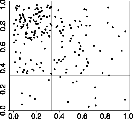
Here, we select sampling locations according to a pattern, such that the locations are more densely clustered in some regions of the domain than others. We consider 200 locations in the unit square which we split into nine subsquares of equal area, see Figure 1. We randomly select 100 points in the top left square and 25 points in the three areas to which it is adjacent. The remaining five subsquares have five points randomly chosen within.

Figure 1. Patterned sampling locations. 100 top left; 25 in top middle, middle left, and middle middle; five top right, middle right, and bottom third. We use the points shown here to analyze the effect of the sampling locations on the spatially varying weights, see Figure 2.

We consider^{Figure 3, Figure 4, Figure 5}five variance ratios: δ₀ = σ²₀/σ²_ε = 0.01, 0.1, 1, 10, 100, and three effective ranges: $d_0=\sqrt{2}/3,2\sqrt{2}/3,\sqrt{2}$, which are chosen with respect to the maximum separation of two points in the unit square, $\sqrt{2}$. An effective range of zero, implying independent random effects, returns weights that are the same at each location. For each of the 15 variance ratio-effective range combinations we compute $\mathbf{W}{\mathbf{X}}_2$, whose ith value is the weight assigned to θ₀ at each ${\mathbf{s}}_i$ i = 1, …, 200.

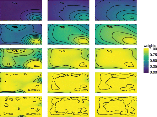
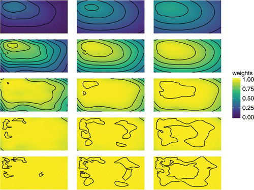
We use the interp() function in the R package akima (Akima and Gebhardt 2016) to interpolate the weights over the unit square. These interpolated plots of spatially varying weights are given in Figure 2 and are created in ggplot2 (Wickham 2009), making use of the ‘gather()’ function in tidyr (Wickham 2017) to set up the data frame. Each row corresponds to a value of δ₀, from 0.01 in top row to 100 in the bottom. For each row going left to right, we have increasing effective ranges, $d_0=\sqrt{2}/3,2\sqrt{2}/3,\sqrt{2}$. We can see that as the variance ratio increases the weights are higher, as they are when the effective range increases. Within each panel, the areas of higher weights are concentrated around the areas of more densely positioned sampling locations. The stronger the correlation, the farther reaching is the influence of these clusters.

Figure 2. Interpolated surfaces of weights for the PCP for 15 combinations of variance ratio δ₀ and effective range d₀. Rows correspond to five values of δ₀ = 0.01, 0.1, 1, 10, 100, increasing top to bottom. Columns correspond to three values of $d_0=\sqrt{2}/3,2\sqrt{2}/3,\sqrt{2}$, increasing left to right. The plot shows that the optimal parameterization gives greater weight to the CP where sampling locations are more densely clustered.

3.2. A Spatially Varying Slope Model

We now investigate the effect of a covariate upon the spatially varying weights. To do this we look at the following model: (13) $$\begin{array}{ccc}\hfill \mathbf{Y}\mid {\mathbf{\beta }}_1^w,{\theta }_1& \sim & N\left\{\mathbf{D}{\mathbf{\beta }}_1^w+(\mathbf{I}-\mathbf{W})\mathbf{1}{\theta }_1,{\sigma }_{ϵ}^2\mathbf{I}\right\},\hfill \\ \hfill {\mathbf{\beta }}_1^w\mid {\theta }_1& \sim & N\left(\mathbf{W}\mathbf{1}{\theta }_1,{\sigma }_1^2{\mathbf{R}}_1\right),\hfill \end{array}$$(13) θ₁ ∼ N(m₁, σ²₁v₁), where $\mathbf{D}=\text{diag}\left(\mathbf{x}\right)$ and $\mathbf{x}={\{x\left({\mathbf{s}}_1\right),\dots ,x\left({\mathbf{s}}_n\right)\}}^{\mathrm{T}}$ contains the values of a known spatially referenced covariate. We have a global slope, hence $\mathbf{\theta }={\theta }_1,$ and a partially centered spatial process ${\mathbf{\beta }}^w={\mathbf{\beta }}_1^w$. Model (13(13) $$\begin{array}{ccc}\hfill \mathbf{Y}\mid {\mathbf{\beta }}_1^w,{\theta }_1& \sim & N\left\{\mathbf{D}{\mathbf{\beta }}_1^w+(\mathbf{I}-\mathbf{W})\mathbf{1}{\theta }_1,{\sigma }_{ϵ}^2\mathbf{I}\right\},\hfill \\ \hfill {\mathbf{\beta }}_1^w\mid {\theta }_1& \sim & N\left(\mathbf{W}\mathbf{1}{\theta }_1,{\sigma }_1^2{\mathbf{R}}_1\right),\hfill \end{array}$$(13) ) can be retrieved from model (4(4) $$\begin{array}{ccc}\hfill \mathbf{Y}\mid {\mathbf{\beta }}^w,\mathbf{\theta }& \sim & N\{{\mathbf{X}}_1{\mathbf{\beta }}^w+{\mathbf{X}}_1(\mathbf{I}-\mathbf{W}){\mathbf{X}}_2\mathbf{\theta },{\mathbf{C}}_1\},\hfill \\ \hfill {\mathbf{\beta }}^w\mid \mathbf{\theta }& \sim & N(\mathbf{W}{\mathbf{X}}_2\mathbf{\theta },{\mathbf{C}}_2),\mathbf{\theta }\sim N(\mathbf{m},{\mathbf{C}}_3),\hfill \end{array}$$(4) ) by letting ${\mathbf{X}}_1=\mathbf{D}$, ${\mathbf{C}}_1={\sigma }_{ϵ}^2\mathbf{I}$, ${\mathbf{X}}_2=\mathbf{1}$, ${\mathbf{C}}_2={\sigma }_1^2{\mathbf{R}}_1$, $\mathbf{m}=m_1$ and ${\mathbf{C}}_3={\sigma }_1^2{v}_1$.

For model (13(13) $$\begin{array}{ccc}\hfill \mathbf{Y}\mid {\mathbf{\beta }}_1^w,{\theta }_1& \sim & N\left\{\mathbf{D}{\mathbf{\beta }}_1^w+(\mathbf{I}-\mathbf{W})\mathbf{1}{\theta }_1,{\sigma }_{ϵ}^2\mathbf{I}\right\},\hfill \\ \hfill {\mathbf{\beta }}_1^w\mid {\theta }_1& \sim & N\left(\mathbf{W}\mathbf{1}{\theta }_1,{\sigma }_1^2{\mathbf{R}}_1\right),\hfill \end{array}$$(13) ) the $\mathbf{W}$ matrix is $\mathbf{W}={\sigma }_1^2{\mathbf{R}}_1\mathbf{D}{({\sigma }_{ϵ}^2\mathbf{I}+{\sigma }_1^2\mathbf{D}{\mathbf{R}}_1\mathbf{D})}^{-1}\mathbf{D}.$ To investigate how these weights vary across the domain we randomly select 200 points uniformly over the unit square. We generate the values of $\mathbf{x}$ by selecting a point ${\mathbf{s}}_x$, which we may imagine to be the site of a source of pollution. We assume that the value for the observed covariate at site ${\mathbf{s}}_i$ decays exponentially at rate φ_x with increasing separation from ${\mathbf{s}}_x$, so that $x\left({\mathbf{s}}_i\right)=exp(-{\varphi }_x\parallel {\mathbf{s}}_i-{\mathbf{s}}_x\parallel )$ for i = 1, …, n. The spatial decay parameter φ_x is chosen such that there is an effective spatial range of $\sqrt{2}/2$, that is, if $\parallel {\mathbf{s}}_i-{\mathbf{s}}_x\parallel =\sqrt{2}/2$ then $x\left({\mathbf{s}}_i\right)=0.05$. 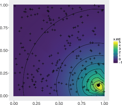The values of $\mathbf{x}$ are standardized by subtracting their sample mean and dividing by their sample standard deviation. Figure 3 gives the interpolated covariate surface where ${\mathbf{s}}_x={(0.936,0.117)}^{\mathrm{T}}$. We can see how the values decay with increased separation from ${\mathbf{s}}_x$.

Figure 3. Interpolated surface of $\mathbf{x}$ from the 200 uniformly sampled data locations, given by ’+’. The values of $\mathbf{x}$ decay with distance from the source, represented by a black dot. We use $\mathbf{x}$ to analyze the effect of covariates on the spatially varying weights for the PCP, see Figure 4.

The optimal weights are computed for 15 combinations of variance ratio δ₁ and effective range d₁, where δ₁ = σ²₁/σ²_ε = 0.01, 0.1, 1, 10, 100 and $d_1=\sqrt{2}/3$, $2\sqrt{2}/3,\sqrt{2}$. The weights are interpolated and illustrated in Figure 4. The weights increase with increasing δ₁ or d₁. It is also evident that for locations near ${\mathbf{s}}_x$, where the values of the covariate are greatest, the weights are higher.

Figure 4. Interpolated weights for the PCP for 15 combinations of δ₁ and d₁. Rows correspond to five values of δ₀ = 0.01, 0.1, 1, 10, 100, increasing top to bottom. Columns correspond to three values of $d_0=\sqrt{2}/3,2\sqrt{2}/3,\sqrt{2}$, increasing left to right. Weights are greatest where the value of $\mathbf{x}$ is at its greatest, see Figure 3.

4. Simulation Studies

4.1. Simulation Example 1

In this section, we use simulated data to investigate the performance of the Gibbs sampler associated with the PCP. All of the relevant posterior distributions can be found in Appendix A.6 in supplementary materials. We simulate data from model (11(11) $$\begin{array}{ccc}\hfill \mathbf{Y}\mid {\mathbf{\beta }}_0^w,{\theta }_0& \sim & N\left\{{\mathbf{\beta }}_0^w+(\mathbf{I}-\mathbf{W})\mathbf{1}{\theta }_0,{\sigma }_{ϵ}^2\mathbf{I}\right\},\hfill \\ \hfill {\mathbf{\beta }}_0^w\mid {\theta }_0& \sim & N\left(\mathbf{W}\mathbf{1}{\theta }_0,{\sigma }_0^2{\mathbf{R}}_0\right),{\theta }_0\sim N\left(m_0,{\sigma }_0^2{v}_0\right).\hfill \end{array}$$(11) ) for n = 40 randomly chosen locations across the unit square. We let hyperparameters m₀ = 0 and v₀ = 10⁴.

We set θ₀ = 0 and generate data with five variance parameter ratios such that δ₀ = σ²₀/σ²_ε = 0.01, 0.1, 1, 10, 100. This is done by letting σ²₀ = 1 and varying σ²_ε accordingly. For each of the five levels of δ₀ we have four values of the decay parameter φ₀, chosen such that there is an effective range, d₀, of 0, $\sqrt{2}/3$, $2\sqrt{2}/3,$ and $\sqrt{2}$, where $\sqrt{2}$ is the maximum possible separation of two points in the unit square. Hence, there are 20 combinations of σ²₀, σ²_ε and φ₀ in all. Each of these combinations is used to simulate 20 datasets, and so there are 400 datasets in total.

To begin the variance parameters, σ²₀ and σ²_ε, and the decay parameter φ₀ = −log (0.05)/d₀ are held fixed at their true values and so for each iteration of the Gibbs sampler we generate samples from the full conditional distributions of ${\mathbf{\beta }}_0^w$ and θ₀.

The efficiency of the sampler is judged by two measures, both of which are calculated using functions within the R package coda Plummer et al. (2006). The first statistic we use is based on the potential scale reduction factor (PSRF) (Gelman and Rubin 1992). We define the PSRF_M(1.1) to be the number of iterations required for the upper limit of the 95 % confidence interval of the PSRF to fall below 1.1 for the first time.

To compute the PSRF_M(1.1), we simulate multiple chains from widely dispersed starting values. In particular, we take values that are outside of the intervals described by pilot chains. At every fifth iteration, the PSRF is calculated and the number of iterations for its value to drop below 1.1 is the value that we record. The second statistic we use is the effective sample size (ESS) of θ₀, (Robert and Casella 2004, chap. 12).

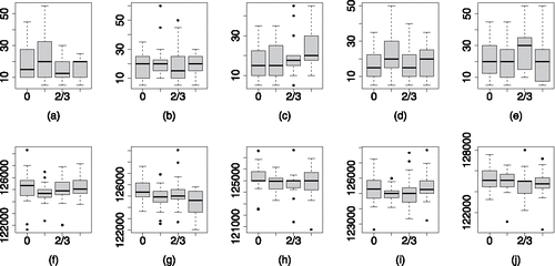
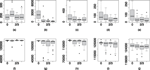
For each dataset, we generate five chains of length 25,000 and compute the PSRF_M(1.1) and the ESS of θ₀ out of a total of 125,000 samples. The results are plotted in Figure 5. On the top row, we have the PSRF_M(1.1) and on the bottom the ESS. The five panels in each row correspond to values of δ₀ = 0.01, 0.1, 1, 10, 100 from left to right and within each panel we have four boxplots, one for each level of the effective range 0, $\sqrt{2}/3$, $2\sqrt{2}/3$ and $\sqrt{2}$. Each boxplot consists of 20 values, for the 20 repetitions of that variance ratio-effective range combination. The figure shows that for the PCP with known variance parameters we achieve near immediate convergence and independent samples for θ₀ in all cases, and that it is robust to changes in both variance ratio and strength of correlation. In some instances, we observe an ESS greater than the total number of samples. This occurs when the estimate of the integrated autocorrelation time is less than zero, which is theoretically possible; see, for example, Besag and Green (1993).

Figure 5. PSRF_M(1.1), panels (a)–(e), and the ESS, panels (f)–(j), of θ₀ for the PCP with known variance parameters. The plots show that the performance of the PCP is insensitive to values of the variance and spatial decay parameters.

4.2. Simulation Example 2

The second simulation study drops the assumption of known variance parameters, fixing only the decay parameter. In this case, we judge performance by the MPSRF_M(1.1) which we define to be the number of iterations needed for the multivariate PSRF (Brooks and Gelman 1998) to fall below 1.1 for the first time. Note that the MPSRF is approximate upper bound to the maximum of the univariate PRSF’s over all monitored variables, see (Brooks and Gelman 1998), Lemma 3. In addition, we record the ESS of θ₀, σ²₀ and σ²_ε.

Recall that variance parameters are given inverse gamma prior distributions with π(σ²₀) = IG(a₀, b₀) and π(σ²_ε) = IG(a_ε, b_ε). We let a₀ = a_ε = 2 and b_ε = b_ε = 1, implying a prior mean of one and infinite prior variance for σ²₀ and σ²_ε. These are common hyperparameters for inverse gamma prior distributions, see Sahu, Gelfand, and Holland (2010, 2007), Gelfand et al. (2003).

Figure 6 shows the MPSRF_M(1.1) on the top row and the ESS of θ₀ on the bottom row for the 20 combinations of δ₀ and d₀ as in the case of Figure 5. There is more variability in the results seen here for the MPSRF_M(1.1) than we saw for the PSRF_M(1.1) when the variance parameters were fixed, Figure 5. When the random effects are independent, weak identifiability of the variance parameters can effect the performance of the sampler as marginally $\mathrm{var}\left\{Y\left({\mathbf{s}}_i\right)\right\}={\sigma }_{ϵ}^2+{\sigma }_0^2$. However, the robustness to changes in δ₀ remains and we still see rapid convergence in most cases. The ESS for θ₀ remains high, with a median value above 120,000 for all of the 20 combinations of δ₀ and d₀.

Figure 6. MPSRF_M(1.1), panels (a)–(e), and the ESS panels (f)–(j), of θ₀ for the PCP with unknown variance parameters. Now, we are updating the parameterization within the sampler, but performance is still good and insensitive to the values of the variance and spatial decay parameters.

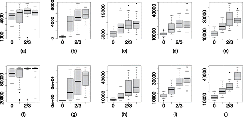
Boxplots of the ESS of the variance parameters are given in Figure 7, with the results^{Table 1}for σ²₀ on the top row and σ²_ε on the bottom row. There is a suggestion that increasing δ₀ increases the ESS of σ²₀ and decreases the ESS of σ²_ε. For a fixed value of δ₀, we can see that the ESS of both variance parameters increases as the effective range increases. The stronger correlation across the random effects means that the variability seen in the data can be more easily separated between the two components.

Figure 7. ESS of σ²₀, panels (a)–(e), and σ²_ε, panels (f)–(j) for the PCP with unknown variance parameters. The ESS of the variance parameters is not strongly effected by their ratio but does improve with stronger spatial correlation.

We compare the results for the PCP with those obtained for the CP and the NCP by calculating the mean responses of each measure of performance for each of the 20 variance ratio-effective range combinations. Table 1 shows the mean MPSRF_M(1.1) and mean ESS for θ₀. The sampling efficiency of the CP and the NCP is dependent on the covariance parameters. The CP performs best for higher values of δ₀ and longer effective ranges, and the NCP performs best for lower values of δ₀ and shorter effective ranges. In contrast, the PCP is robust to changes in δ₀ and d₀. Moreover, we see that the PCP has a lower average MPSRF_M(1.1) for most cases, and when it does not, the difference is less than 3%. It is clear that, in terms of the ESS of θ₀, the PCP is superior to the CP and the NCP in all cases.

Table 1. Means of the MPSRF_M(1.1) and the ESS of θ₀ for 20 variance ratio-effective range combinations for the CP, the NCP and the PCP.

		MPSRFM(1.1)			ESS of θ0
δ0	$d_0/\sqrt{2}$	CP	NCP	PCP	CP	NCP	PCP
0.01	0	3064.50	172.00	163.25	463	108819	124988
	1/3	1115.75	278.25	251.25	1821	103342	116659
	2/3	544.50	166.25	154.00	3055	105397	125108
	1	366.50	184.75	175.00	4652	94657	123730
0.1	0	3528.25	3455.50	2464.50	4707	20420	125272
	1/3	607.00	1305.50	624.25	13336	33347	108922
	2/3	271.25	592.75	251.50	25884	28959	109987
	1	211.00	518.25	203.75	31938	22361	113191
1	0	274.50	910.50	187.50	25523	7353	124945
	1/3	134.50	1639.00	118.75	65927	3785	120325
	2/3	78.25	2092.00	76.00	82100	3148	121013
	1	101.00	2473.75	103.00	84742	2722	115700
10	0	123.50	1140.25	105.75	32578	5226	125091
	1/3	79.75	1556.25	79.75	83586	2918	123055
	2/3	45.25	2824.25	44.50	102306	1734	124341
	1	49.50	3542.25	50.50	107261	1177	122774
100	0	104.75	1124.75	102.75	32891	4596	125388
	1/3	42.75	1607.50	42.50	84755	2772	124120
	2/3	41.75	2544.75	41.50	104941	1671	124214
	1	32.75	3427.75	33.00	108050	1186	124670

The ESS of the variance parameters is not strongly effected by the fitting methods we consider here as a reparameterization only acts upon the mean structure of the model. However, in cases where a particular parameterization is very inefficient, for example, for the NCP when δ₀ > 1, poor mixing can occur for the variance parameters.

5. London Air Pollution Modeling Example

In this section, we compare the efficiency of the CP, the NCP and the PCP when fitting model (1(1) $$\begin{array}{ccc}\hfill Y\left({\mathbf{s}}_i\right)& =& {\theta }_0+{\beta }_0\left({\mathbf{s}}_i\right)+\sum _{k=1}^{p-1}\{{\theta }_k+{\beta }_k\left({\mathbf{s}}_i\right)\}{x}_k\left({\mathbf{s}}_i\right)+ϵ\left({\mathbf{s}}_i\right),\hfill \\ & & i=1,\dots ,n.\hfill \end{array}$$(1) ) to a dataset of NO₂ concentration levels, downloaded from www.londonair.org.uk, for the city of Greater London. 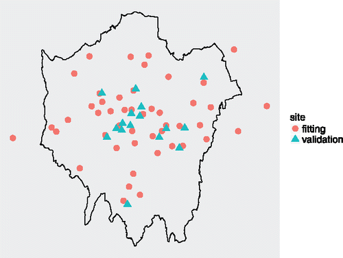It is a spatial dataset with values, in microgram per cubic metre ($\mu \text{g}/{\text{m}}^3$), of the annual mean concentration for the year 2011. Data have been collected at 63 irregularly spaced locations across London. We fit the model using data from 47 sites, leaving out 16 sites for validation (see Figure 8). The mean and standard deviation for the 47 data sites is 81.8 $\mu \text{g}/{\text{m}}^3$ and 38.7 $\mu \text{g}/{\text{m}}^3,$ respectively. This annual mean value is quite high compared to the annual limit value of 40 $\mu \text{g}/{\text{m}}^3$, which has been stated in the national air quality objectives.¹ This objective has been in place since 2005 and so was in effect prior to the collection of these data. Also, note that there is considerable variability in the data as is evident by the high value of the standard deviation.

Figure 8. Sampling locations for NO₂ concentration data.

The spatially varying covariate we use is output from the Air Quality Unified Model (AQUM), a numerical model giving air pollution predictions at 1-km grid cell resolution (Savage et al. 2013). The AQUM is used as a covariate in the model, where $x\left(\mathbf{s}\right)$ is the AQUM output for the grid cell containing s. Therefore, we use a downscaler model as employed by Berrocal, Gelfand, and Holland (2010).

As we have a spatially varying coefficient we fit the different parameterizations of model (1(1) $$\begin{array}{ccc}\hfill Y\left({\mathbf{s}}_i\right)& =& {\theta }_0+{\beta }_0\left({\mathbf{s}}_i\right)+\sum _{k=1}^{p-1}\{{\theta }_k+{\beta }_k\left({\mathbf{s}}_i\right)\}{x}_k\left({\mathbf{s}}_i\right)+ϵ\left({\mathbf{s}}_i\right),\hfill \\ & & i=1,\dots ,n.\hfill \end{array}$$(1) ) with p = 2. Therefore, we have two spatial processes, an intercept and a slope process and so $\tilde{\mathbf{\beta }}={({\tilde{\mathbf{\beta }}}_0^{\mathrm{T}},{\tilde{\mathbf{\beta }}}_1^{\mathrm{T}})}^{\mathrm{T}}$ for the CP, $\mathbf{\beta }={({\mathbf{\beta }}_0^{\mathrm{T}},{\mathbf{\beta }}_1^{\mathrm{T}})}^{\mathrm{T}}$ for the NCP and ${\mathbf{\beta }}^w={({\mathbf{\beta }}_0^{w\mathrm{T}},{\mathbf{\beta }}_1^{w\mathrm{T}})}^{\mathrm{T}}$ for the PCP. Each process has a corresponding global parameter and a variance parameter and so $\mathbf{\theta }={({\theta }_0,{\theta }_1)}^{\mathrm{T}}$ and ${\mathbf{\sigma }}^{\mathbf{2}}={({\sigma }_0^2,{\sigma }_1^2)}^{\mathrm{T}}$. We use an exponential correlation function for both processes and so $\mathbf{\varphi }={({\varphi }_0,{\varphi }_1)}^{\mathrm{T}}$. In addition, we have the data variance, σ²_ε, and so we have 2(n + 3) + 1 parameters to estimate for each parameterization.

For the prior distribution of $\mathbf{\theta },$ we let $\mathbf{m}={(0,0)}^{\mathrm{T}}$ and v₀ = v₁ = 10⁴. We let a₀ = a₁ = a_ε = 2 and b₀ = b₁ = b_ε = 1, so that each variance parameter is assigned an IG(2, 1) prior distribution. To stabilise the variance and avoid negative predictions, we model the data on the square root scale, as done by Sahu, Gelfand, and Holland (2007) and Berrocal, Gelfand, and Holland (2010) when modeling ozone concentrations for the US.

As mentioned in Section 2.1, we estimate the spatial decay parameters by performing a grid search over a range of values for φ₀ and φ₁. The estimates are taken to be the pair of values that minimize the prediction error with respect to the validation data. The criteria used to compute the prediction error are the mean absolute prediction error (MAPE), the root mean square prediction error (RMSPE), and the continuous ranked probability score (CRPS), see Gneiting, Balabdaoui, and Raftery (2007) for example.

We select values of φ₀ and φ₁ corresponding to effective ranges of 5, 10, 25, 50, 100 and 250 km. For each of the 36 pairs of spatial decay parameters, we generate a single chain of 25,000 iterations and discard the first 5,000. In this way, the estimates for the spatial decay parameters are ${\widehat{\varphi }}_0=-log(0.05)/5\approx 0.6,\text{and}{\widehat{\varphi }}_1=-log(0.05)/100\approx 0.03$.

For each parameterization, we generate five Markov chains of length 25,000 from the same set widely dispersed starting values. The MPSRF_M(1.1) and the ESS for $\mathbf{\theta }={({\theta }_0,{\theta }_1)}^{\mathrm{T}}$, ${\mathbf{\sigma }}^{\mathbf{2}}={({\sigma }_0^2,{\sigma }_1^2)}^{\mathrm{T}}$ and σ²_ε are^{Figure 9}computed and given in Table 2.

Table 2. MPSRF_M(1.1) and the ESS of the model parameters.

	MPSRFM(1.1)	ESS θ0	ESS θ1	ESS σ^20	ESS σ^21	ESS σ^2ε
PCP	360	120956	121092	5996	7499	20925
CP	460	20548	57177	2279	7578	2452
NCP	1230	15132	4421	2273	5038	2392

In this example, and also previously in the simulation examples, we evaluate the efficiency of the sampling algorithms for the fixed effects and global variance parameters which are of interests for inferential purposes. However, we have also monitored the convergence for a random sample of the spatially varying random effects, $\beta \left(\mathbf{s}\right)$. We did not encounter any problem in their convergence behavior.

We see that the CP requires far fewer iterations for the MPSRF to drop below 1.1 than the NCP, 460 versus 1230. The short effective range for the intercept process means that the ESS for θ₀ is only slightly greater for the CP than the NCP, but due to the stronger spatial association in the regression process the ESS for θ₁ is nearly 13 times greater for the CP than the NCP. However, the PCP, whose performance insensitive to the values of the model parameters, demonstrates extremely low autocorrelation between successive samples with an ESS greater than 120,000 for both θ₀ and θ₁.

The run times for the CP and the NCP are almost the same, but updating $\mathbf{W}$ within the sampler means that the PCP is more computationally demanding. Table 3 gives the same measures as Table 2 but adjusted for computation time. We let $${\text{MPSRF}}_t(1.1)={\text{MPSRF}}_M(1.1)\times \text{time}\text{per}\text{iteration},$$denote the computation time (in seconds) for the MPSRF to fall below 1.1, and let ESS/s denote the ESS per second.

Table 3. MPSRF_t(1.1) and ESS/s of the model parameters.

	MPSRFt(1.1)	ESS/s θ0	ESS/s θ1	ESS/s σ^20	ESS/s σ^21	ESS/s σ^2ε
PCP	6.96	50.06	50.12	2.48	3.10	8.66
CP	4.89	15.47	43.05	1.72	5.71	1.85
NCP	13.07	11.39	3.33	1.71	3.79	1.80

Even accounting for the shorter run times of the CP, the PCP is comparable in terms of MPSRF_t(1.1) and ESS/s of the variance components, but most importantly it is superior in terms of ESS/s for the mean parameters.

Figure 9 shows the spatially varying parameterization that results from the PCP. Contained are interpolated maps of the average weight of partial centering given by each process to each global parameter for all 63 sampling locations. The top row displays the weights given by ${\mathbf{\beta }}_0^w$ to θ₀ on the left, and the weights given by ${\mathbf{\beta }}_1^w$ to θ₁ on the right. To restrict the interpolated weight values within the unit interval (0, 1), we first logit-transform the weights and then use the inverse logit transformation on the interpolated values.

Figure 9. Spatially varying weights for London NO₂ concentration data. On the top row are the weights assigned to the global parameter corresponding to each process. On the left, the weight of θ₀ in the mean of ${\mathbf{\beta }}_0^w$, and on the right the weight of θ₁ in the mean of ${\mathbf{\beta }}_1^w$. The bottom row gives the weights for the alternate global parameter. On the left, the weight of θ₁ in the mean of ${\mathbf{\beta }}_0^w$, and on the right the weight of θ₀ in the mean of ${\mathbf{\beta }}_1^w$.

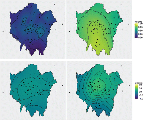
The weights for θ₀ are low; the estimated weights at the data locations (not the interpolated weights) are between 0.11 and 0.38. This reflects the short effective range of the intercept process, which is 5 kilometres (km). The weights for θ₁ are much higher, between 0.50 and 0.88, and this is due to the longer effective range of the slope process, 100 km. The weights vary over the spatial locations and are neither exactly zero or one, which would correspond to the NCP and CP respectively. They are higher where there are clusters of monitoring sites. We see this behavior in Figure 2. It is more clearly demonstrated when there is a shorter effective range as the influence of the clustering of data points is not so far reaching, thus the pattern can be discerned from the plot.

The bottom row displays the weights given by ${\mathbf{\beta }}_0^w$ to θ₁ on the left, and the weight given by ${\mathbf{\beta }}_1^w$ to θ₀ on the right. These take values in (–1, 1) and so we transform them to the unit interval before taking the logit transformation, then the interpolated weights are back-transformed.

When producing the plots, to have Greater London fully contained within the convex hull of the sampling locations, we move the most northerly observation site further north by adding 0.05 to its latitude. In addition to the packages needed to produce Figure 2, we use functions within maptools (Bivand and Lewin-Koh 2016) to handle the shape files and the pointsInPoly function in spBayes to remove those points on the interpolated grid that lie outside of the polygon described by the Greater London Boundary.

6. Discussion

We have investigated the performance of a PCP for the spatially varying coefficients model. We are able to parameterize the model in such a way that we remove the posterior covariance between the random and global effects and produce a Gibbs sampler which converges immediately. The construction is conditioned on the covariance matrices in the model. We have shown that the parameterization can be updated dynamically within the Gibbs sampler for the case when these matrices are known only up to a set of covariance parameters which must be estimated.

The optimal weights of partial centering are shown to vary over the spatial domain, with higher weights given to locations where the data are more informative about the latent surface. Therefore, higher weights are found when the data precision is relatively high, or there is some clustering of locations. We also saw higher weights for locations where the value of the covariate was higher.

We make it clear that although the interpolated plots given in Sections 3 and 5 are informative they do not represent a true surface in the sense that the interpolated values are not estimates of a true value of the weights at an unsampled location. Indeed, if we were to obtain a further measurement at a new location then the values of the weights at the existing locations would change.

Our investigations show that the unlike the CP and the NCP, the performance of the PCP is robust to changes in the variance and correlation parameters. Swift convergence and independent, or near independent samples from the posterior distributions of the mean parameters are achieved for all of the datasets we considered, whether it was simulated or real data.

The PCP requires us to update all of the random effects in one block and all of the global effects in another. It is a computationally intensive strategy which we recommend for modest sized spatial datasets. However, for larger datasets many practitioners turn to Gaussian predictive process approximations, as implemented in R software packages spBayes (Finley, Banerjee, and Gelfand 2015) and spTimer (Bakar and Sahu 2015). As the method proposed in this article, can be applied to any model that can be written as a three stage NLHM, we believe that the PCP could be used in conjunction with GPP models thus broadening its applicability. We also note that PCP can be used for the Generalized linear models incorporating spatially varying random effects.

Acknowledgments

This research was supported in part by the EPSRC research grant EP/J017485/1 awarded to the correspinding author. Much of this work was completed when the first author was a PhD student in the University of Southampton. The authors thank the referees for helpful comments.

Supplementary Materials

	Appendices: A.1 to A.6 containing proofs and further details as referenced in the main article.
	C code: All of the C code used to generate the MCMC output which is analyzed to produce the results given in this article are contained within the folder called c_files. Full details are provided within the README.txt file contained within the folder.
	Data: All data files can be found in the folder labeled data_files. A full description is given in the README.txt file contained therein.
	R code: The R code used to analyze the MCMC output produced by the C code can be found in the folder labeled R_scripts. A full description of the files is given in README.txt.
	Figures: The figures produced by the R code included in this article are given in the folder labeled figures.

Notes

1 https://uk-air.defra.gov.uk/air-pollution/uk-eu-limits, last modified March 3, 2017

References

- Akima, H., and Gebhardt, A. (2016), “akima: Interpolation of Irregularly and Regularly Spaced Data,” R package version 0.6-2.
- Bakar, K. S., and Sahu, S. K. (2015), “spTimer: Spatio-Temporal Bayesian Modeling Using R,” Journal of Statistical Software, 63, 1–32.
- Bass, M. R., and Sahu, S. K. (2017), “A Comparison of Centring Parameterisations of Gaussian Process-Based Models for Bayesian Computation using MCMC,” Statistics and Computing, 27, 1491–1512.
- Berrocal, V. J., Gelfand, A. E., and Holland, D. M. (2010), “A Spatio-Temporal Downscaler for Output from Numerical Models,” Journal of Agricultural, Biological, and Environmental statistics, 15, 176–197.
- Besag, J., and Green, P. J. (1993), “Spatial Statistics and Bayesian Computation” (with discussion), Journal of the Royal Statistical Society, Series B, 55, 25–37.
- Bivand, R., and Lewin-Koh, N. (2016), “maptools: Tools for Reading and Handling Spatial Objects,” R package version 0.8-39.
- Brooks, S. P., and Gelman, A. (1998), “General Methods for Monitoring Convergence of Iterative Simulations,” Journal of Computational and Graphical Statistics, 7, 434–455.
- Cressie, N., and Johannesson, G. (2008), “Fixed Rank Kriging for very Large Spatial Data Sets,” Journal of the Royal Statistical Society, Series B, 70, 209–226.
- Finley, A. O., Banerjee, S., and Gelfand, A. E. (2015), “spBayes for Large Univariate and Multivariate Point-Referenced Spatio-Temporal Data Models,” Journal of Statistical Software, 63, 1–28.
- Finley, A. O., Banerjee, S., and MacFarlane, D. W. (2011), “A Hierarchical Model for Quantifying Forest Variables over Large Heterogeneous Landscapes with Uncertain Forest Areas,” Journal of the American Statistical Association, 106, 31–48.
- Gelfand, A. E., Kim, H.-J., Sirmans, C., and Banerjee, S. (2003), “Spatial Modeling with Spatially Varying Coefficient Processes,” Journal of the American Statistical Association, 98, 387–396.
- Gelfand, A. E., Sahu, S. K., and Carlin, B. P. (1995), “Efficient Parameterisations for Normal Linear Mixed Models,” Biometrika, 82, 479–488.
- Gelfand, A. E., and Smith, A. F. (1990), “Sampling-Based Approaches to Calculating Marginal Densities,” Journal of the American Statistical Association, 85, 398–409.
- Gelman, A., and Rubin, D. B. (1992), “Inference from Iterative Simulation using Multiple Sequences,” Statistical Science, 7, 457–472.
- Gneiting, T., Balabdaoui, F., and Raftery, A. E. (2007), “Probabilistic Forecasts, Calibration and Sharpness,” Journal of the Royal Statistical Society, Series B, 69, 243–268.
- Hamm, N., Finley, A., Schaap, M., and Stein, A. (2015), “A Spatially Varying Coefficient Model for Mapping PM10 Air Quality at the European Scale,” Atmospheric Environment, 102, 393–405.
- Handcock, M. S., and Stein, M. L. (1993), “A Bayesian Analysis of Kriging,” Technometrics, 35, 403–410.
- Harville, D. A. (1997), Matrix Algebra from a Statistician’s Perspective, New York: Springer-Verlag.
- Huerta, G., Sansó, B., and Stroud, J. R. (2004), “A Spatio-temporal Model for Mexico City ozone Levels,” Journal of the Royal Statistical Society, Series C, 53, 231–248.
- Matérn, B. (1986), Spatial Variation (2nd ed.), Berlin: Springer Verlag.
- Papaspiliopoulos, O. (2003), “Non-Centered Parameterisations for Data Augmentation and Hierarchical Models with Applications to Inference for Lévy-Based Stochastic Volatility Models,” Ph.D. thesis, University of Lancaster.
- Papaspiliopoulos, O., Roberts, G. O., and Sköld, M. (2003), “Non-centered parameterisations for hierarchical models and data augmentation (with discussion),” in Bayesian Statistics 7 (Bernardo, JM and Bayarri, MJ and Berger, JO and Dawid, AP and Heckerman, D and Smith, AFM and West, M): Proceedings of the Seventh Valencia International Meeting, Oxford University Press, USA, pp. 307–326.
- Plummer, M., Best, N., Cowles, K., and Vines, K. (2006), “CODA: Convergence Diagnosis and Output Analysis for MCMC,” R News, 6, 7–11.
- R Core Team (2016), R: A Language and Environment for Statistical Computing, Vienna, Austria: R Foundation for Statistical Computing.
- Robert, C. O., and Casella, G. (2004), Monte Carlo Statistical Methods” (2nd ed.), New York: Springer-Verlag.
- Sahu, S. K., Gelfand, A. E., and Holland, D. M. (2007), “High-Resolution Space–Time Ozone Modeling for Assessing Trends,” Journal of the American Statistical Association, 102, 1221–1234.
- ——— (2010), “Fusing Point and Areal Level Space–Time Data with Application to Wet Deposition,” Journal of the Royal Statistical Society, Series C, 59, 77–103.
- Savage, N., Agnew, P., Davis, L., Ordóñez, C., Thorpe, R., Johnson, C., O’Connor, F., and Dalvi, M. (2013), “Air Quality Modelling using the Met Office Unified Model (AQUM OS24-26): Model Description and Initial Evaluation,” Geoscientific Model Development, 6, 353–372.
- Wheeler, D. C., Páez, A., Spinney, J., and Waller, L. A. (2014), “A Bayesian Approach to Hedonic Price Analysis,” Papers in Regional Science, 93, 663–683.
- Wickham, H. (2009), ggplot2: Elegant Graphics for Data Analysis, New York: Springer-Verlag.
- ——— (2017), “tidyr: Easily Tidy Data with ‘spread()’ and ‘gather()’ Functions,” R package version 0.6.1.
- Yu, Y., and Meng, X.-L. (2011), “To Center or Not to Center: That is Not the Question: An Ancillarity–Sufficiency Interweaving Strategy (ASIS) for Boosting MCMC Efficiency,” Journal of Computational and Graphical Statistics, 20, 531–570.
- Zhang, H. (2004), “Inconsistent Estimation and Asymptotically Equal Interpolations in Model-Based Geostatistics,” Journal of the American Statistical Association, 99, 250–261.