Adaptive Incremental Mixture Markov Chain Monte Carlo

Abstract

We propose adaptive incremental mixture Markov chain Monte Carlo (AIMM), a novel approach to sample from challenging probability distributions defined on a general state-space. While adaptive MCMC methods usually update a parametric proposal kernel with a global rule, AIMM locally adapts a semiparametric kernel. AIMM is based on an independent Metropolis–Hastings proposal distribution which takes the form of a finite mixture of Gaussian distributions. Central to this approach is the idea that the proposal distribution adapts to the target by locally adding a mixture component when the discrepancy between the proposal mixture and the target is deemed to be too large. As a result, the number of components in the mixture proposal is not fixed in advance. Theoretically, we prove that there exists a stochastic process that can be made arbitrarily close to AIMM and that converges to the correct target distribution. We also illustrate that it performs well in practice in a variety of challenging situations, including high-dimensional and multimodal target distributions. Finally, the methodology is successfully applied to two real data examples, including the Bayesian inference of a semiparametric regression model for the Boston Housing dataset. Supplementary materials for this article are available online.

Keywords:

• Adaptive MCMC
• Bayesian inference
• Importance weight
• Independence sampler
• Local adaptation

1 Introduction

We consider the problem of sampling from a target distribution defined on a general state space. While standard simulation methods such as the Metropolis–Hastings algorithm (Metropolis et al. 1953; Hastings 1970) and its many variants have been extensively studied, they can be inefficient in sampling from complex distributions such as those that arise in modern applications. For example, the practitioner is often faced with the issue of sampling from distributions which contain some or all of the following: multimodality, very nonelliptical high density regions, heavy tails, and high-dimensional support. In these cases, standard Markov chain Monte Carlo (MCMC) methods often face difficulties: long mixing time and large asymptotic variance leading to potentially biased and large variance MCMC estimators. Adaptive Monte Carlo methods, which can be traced back to Gilks, Roberts, and George (1994), can help overcome these problems. In the specific context of MCMC algorithms, the seminal works are Gilks, Roberts, and Sahu (1998) and Haario, Saksman, and Tamminen (1999). The theoretical properties of these algorithms have been extensively analyzed by Andrieu and Moulines (2006) and Roberts and Rosenthal (2007). Adaptive MCMC methods improve the convergence of the chain by tuning its transition kernel on the fly using knowledge of the past trajectory of the process. This learning process causes a loss of the Markovian property and the resulting stochastic process is therefore no longer a Markov chain.

Most of the adaptive MCMC literature to date has focused on updating an initial parametric proposal distribution. For example, the adaptive Metropolis–Hastings algorithm (Haario, Saksman, and Tamminen 1999, 2001), hereafter referred to as AMH, adapts the covariance matrix of a Gaussian proposal kernel, used in a random walk Metropolis–Hastings algorithm. The adaptive Gaussian mixtures algorithm (Giordani and Kohn 2010; Luengo and Martino 2013), hereafter referred to as AGM, adapts a mixture of Gaussian distributions, used as the proposal in an independent Metropolis–Hastings algorithm.

When knowledge on the target distribution is limited, the assumption that a good proposal kernel can be found in a specific parametric family may lead to suboptimal performance. Indeed, a practitioner using these methods must choose, sometimes arbitrarily, (i) a parametric family and (ii) an initial set of parameters to start the sampler. However, poor choices of (i) and (ii) may hamper the adaptation and result in slow convergence.

In this article, we introduce a novel adaptive MCMC method, called adaptive incremental mixture Markov chain Monte Carlo (AIMM). This algorithm belongs to the general adaptive independent Metropolis class of methods, developed in Holden, Hauge, and Holden (2009), in that AIMM adapts an independence proposal density. However, the adaptation process here is quite different from others previously explored in the literature. Although our objective remains to reduce the discrepancy between the proposal and the target distribution along the chain, AIMM proceeds without any global parameter updating scheme, as is the case with adaptive MCMC methods belonging to the framework developed in Andrieu and Moulines (2006).

Our idea is instead to add a local probability mass to the current proposal kernel, when a large discrepancy between the target and the proposal is encountered. The local probability mass is added through a Gaussian kernel located in the region that is not sufficiently supported by the current proposal. The decision to increment the proposal kernel is based on the importance weight function that is implicitly computed in the Metropolis acceptance ratio. We stress that, although seemingly similar to Giordani and Kohn (2010) and Luengo and Martino (2013), our adaptation scheme is local and semiparametric since the number of mixture components is not specified, a subtle difference that has important theoretical and practical consequences. In particular, in contrast to AGM, the approach which we develop does not assume a fixed number of mixture components. The AIMM adaptation strategy is motivated by the quantitative bounds achieved when approximating a density using the recursive mixture density estimation algorithm proposed in Li and Barron (2000). The main difference is that while in AIMM the sequence of proposals is driven by the importance weight function at locations visited by the AIMM Markov chain, it is constructed in Li and Barron (2000) by successively minimizing the entropy with respect to the target distribution, an idea which was also put forward in Cappé et al. (2008). In fact, the AIMM adaptation strategy shares perhaps more similarity with the adaptive rejection Metropolis sampler (ARMS) from Gilks, Best, and Tan (1995) which is an MCMC extension of ARS (Gilks and Wild 1992). In unidimensional settings, the ARMS proposal is a piecewise exponential density which essentially interpolates the set of accepted and rejected samples of an independent MH. More recent works have developed different adaptation schemes with other nonparametric densities: piecewise triangular or trapezoidal functions (Cai, Meyer, and Perron 2008) and Lagrange interpolation polynomials (Meyer, Cai, and Perron 2008). The ARMS algorithm has been improved in Martino, Read, and Luengo (2015) where the authors also use the notion of importance weight to adapt the set of points used to build the proposal density. We refer to Martino et al. (2018) for a thorough review of those methods. The main drawback of those methods is that, even though Metropolis-within-Gibbs versions of those algorithms can be considered, they are essentially designed for unidimensional problems. Our work is inspired by the efficiency of those univariate nonparametric adaptation schemes which we combine with the high-dimensional flexibility offered by the mixture of Gaussian kernels.

As in most adaptive MCMC, AIMM requires the specification of some tuning parameters and in particular the threshold parameter controlling the tolerated discrepancy between the target distribution and the adaptive proposal. Although we are not able to prove any optimality result regarding those parameters, we provide a default setting that works well empirically in the examples we have considered and some heuristics that automate these choices. At a more general level, we anticipate that this work will be used by practitioners as a basis for their own inference problem. In this spirit, we also present a faster version of AIMM that guarantees that the proposal is not too costly to evaluate, a situation which occurs when the number of components in the incremental mixture gets large, especially if the state space is high dimensional.

Proving the ergodicity of adaptive MCMC methods is often made easier by expressing the adaptation as a stochastic approximation process consisting of the proposal kernel parameters (Andrieu and Moulines 2006). AIMM cannot be analyzed in this framework as the adaptation does not proceed with a global parameter update step. We do not study the ergodicity of the process in the framework developed by Holden, Hauge, and Holden (2009), and also used in Giordani and Kohn (2010), as the Doeblin condition required there is essentially equivalent to assuming that the importance function is bounded above. This condition is generally hard to meet in most practical applications, unless the state space is finite or compact. Instead, our ergodicity proof relies on the seminal work by Roberts and Rosenthal (2007), which shows that (i) if the process adapts less and less (diminishing adaptation) and (ii) if any Markov kernel used by the process to transition reaches stationarity in a bounded time (containment), then the adaptive process is ergodic. We show that AIMM can be implemented in a way that guarantees diminishing adaptation, while the containment condition remains to be proven on a case by case basis, depending on the target distribution. Moreover, we show using the recent theory developed in Craiu et al. (2015) and Rosenthal and Yang (2017) that there exists a process, which can be made arbitrarily close to the AIMM process, which is ergodic for the target distribution at hand.

The article is organized as follows. We start in Section 2 with a pedagogical example which shows how AIMM succeeds in addressing the pitfalls of some adaptive MCMC methods. In Section 3, we formally present AIMM, and study its theoretical properties in Section 4. Section 5 illustrates the performance of AIMM on some synthetic examples, involving two high-dimensional heavy-tailed distributions and a bimodal distribution. Section 6 presents two successful applications of AIMM on Bayesian inference of real data. We conclude by discussing the connections with importance sampling methods, particularly incremental mixture of importance sampling (Raftery and Bao 2010), from which AIMM takes inspiration, in Section 7.

2 Introductory Example

We first illustrate some of the potential shortcomings of the adaptive methods mentioned in Section 1 and outline how AIMM addresses them. We consider the following pedagogical example where the objective is to sample efficiently from a one-dimensional target distribution.

Example 1.

Consider the target distribution $${\pi }_1=(1/4) \mathcal{N}(-10,1)+(1/2) \mathcal{N}(0,0.1)+(1/4) \mathcal{N}(10,1) .$$

For this type of target distribution it is known that AMH (Haario, Saksman, and Tamminen 2001) mixes poorly since the three modes of ${\pi }_1$ are far apart, a problem faced by many nonindependent Metropolis algorithms. Thus, an adaptive independence sampler such as the AGM (Luengo and Martino 2013) is expected to be more efficient. AGM uses the history of the chain to adapt the parameters of a mixture of Gaussians on the fly to match the target distribution. For AGM, we consider here three families of proposals: the set of mixtures of two, three, and forty Gaussians, referred to as AGM-2, AGM-3, and AGM-40, respectively. The authors recommend initializing AGM proposal with a large number of components and, possibly, resampling the most important components of the proposal. By contrast, our method, AIMM offers more flexibility in terms of the specification of the proposal distributions and in particular does not set a fixed number of mixture components.

We are particularly interested in studying the tradeoff between the convergence rate of the Markov chain and the asymptotic variance of the MCMC estimators, which are known to be difficult to control simultaneously (Mira 2001; Rosenthal 2003). Table 1 gives information about the asymptotic variance, through the effective sample size (ESS), and about the speed of convergence of the chain, through the mean squared error (MSE) of a tail-event probability (defined here as ${\pi }_1(X>5)$). Further details of these performance indicators can be found in the supplementary materials (Section 3).

Table 1 (Example 1) Results for ${\pi }_1$: effective sample size (ESS) (the larger the better), mean squared error (MSE) of ${\pi }_1(X>5)$ (the smaller the better).

	ESS	MSE ($\times {10}^4$)
AMH	$(0.08,0.004)$	6030
AGM-2	$(0.12,0.001)$	120
AGM-3	$(0.51,0.091)$	76
AGM-40	$(0.91,0.008)$	5
AIMM	$(0.47,0.004)$	7

NOTE: Estimates obtained through 100 independent runs of the four methods, each of 20,000 iterations, discarding the first 10,000 iterations for burn in. For the ESS statistic, the mean and variance are provided.

The ability of AMH to explore the state space appears limited as it regularly fails to visit the three modes in their correct proportions after 20,000 iterations (see the MSE of ${\pi }_1(X>5)$ in Table 1). The efficiency of AGM depends strongly on the number of mixture components of the proposal family. In fact AGM-2 is comparable to AMH in terms of the average ESS, indicating that the adaptation failed in most runs. AIMM and AGM-3 both achieve a similar exploration of the state space and AGM-3 offers a slightly better ESS. Finally, AGM-40 outperforms the other methods in this example and it virtually samples iid draws from π. An animation corresponding to this toy example can be found at http://mathsci.ucd.ie/∼fmaire/AIMM/toy_example.html.

From this example we conclude that AGM can be extremely efficient provided some initial knowledge on the target distribution, for example, the number of modes, the location of the large density regions, and so on. If a mismatch between the family of proposal distributions and the target occurs, inference can be jeopardized. Since misspecifications are typical in real world models where one encounters high-dimensional, multimodal distributions, and other challenging situations, it leads one to question the efficiency of AGM samplers. On the other hand, AMH seems more robust to a priori lack of knowledge of the target, but the quality of the mixing of the chain remains a potential issue, especially when high density regions are disjoint.

Initiated with a naive independence proposal, AIMM adaptively builds a proposal that approximates the target iteratively by adding probability mass to locations where the proposal is not well supported relative to the target; see Section 3.6 for details. As a result, very little, if any, information regarding the target distribution is needed. Extensive experimentation in Section 5 confirms this point.

3 Adaptive Incremental Mixture MCMC

We consider target distributions $\pi$ defined on a measurable space $(X,\mathcal{X})$ where $X$ is an open subset of ${\mathbb{R}}^d$ (d > 0) and $\mathcal{X}$ is the Borel σ-algebra of $X$. Unless otherwise stated, the distributions we consider are dominated by the Lebesgue measure and we therefore denote the distribution and the density function (w.r.t the Lebesgue measure) by the same symbol. In this section, we introduce the family of adaptive algorithms referred to AIMM, the acronym for adaptive incremental mixture MCMC.

3.1 Transition Kernel

AIMM belongs to the general class of adaptive independent Metropolis algorithms originally introduced by Gåsemyr (2003) and studied by Holden, Hauge, and Holden (2009). AIMM generates a stochastic process $\{X_n, n\in \mathbb{N}\}$ that induces a collection of independence proposals $\{Q_n, n\in \mathbb{N}\}$. At iteration n, the process is at X_n and attempts a move to ${\tilde{X}}_{n+1}\sim Q_n$ which is accepted with probability α_n. In what follows, $\{{\tilde{X}}_n, n\in {\mathbb{N}}^{\ast }\}$ denotes the sequence of proposed states that are either accepted or rejected.

More formally, AIMM produces a time inhomogeneous process whose transition kernel K_n (at iteration n) is the standard Metropolis–Hastings (MH) kernel with independence proposal Q_n and target $\pi$. For any $(x,A)\in (X,\mathcal{X})$, K_n is defined by (1) $$\begin{array}{c}{K}_n(x;A):={\int }_A{Q}_n(\mathrm{d}x\prime ){\alpha }_n(x,x\prime )\\ +{\delta }_x\left(A\right){\int }_X{Q}_n(\mathrm{d}x\prime )\left(1-{\alpha }_n(x,x\prime )\right) .\end{array}$$(1)

In (1), α_n denotes the usual MH acceptance probability for independence samplers, namely (2) $${\alpha }_n(x,x\prime ):=1\wedge \frac{W_n(x\prime )}{W_n\left(x\right)} ,$$(2) where $W_n:=\pi /Q_n$ is the importance weight function defined on $X$. Central to our approach is the idea that the discrepancy between $\pi$ and Q_n, as measured by W_n, can be exploited to adaptively improve the independence proposal. This has the advantage that W_n is computed as a matter of course in the MH acceptance probability (2).

3.2 Incremental Process

We assume that available knowledge about $\pi$ allows one to construct an initial proposal kernel Q₀, from which it is straightforward to sample. When $\pi$ is a posterior distribution, a default choice for Q₀ could be the prior distribution. The initial proposal Q₀ is assumed to be relatively flat, in the spirit of a defensive distribution (Hesterberg 1995). Initiated at Q₀, a sequence of proposals $\{Q_n, n\in \mathbb{N}\}$ is produced by our algorithm. In particular, the proposal kernel adapts by adding probability mass where the discrepancy between Q_n and $\pi$ is deemed too large.

The adaptation mechanism is driven by the random sequence $\{W_n({\tilde{X}}_{n+1}), n\in \mathbb{N}\}$, which monitors the discrepancy between $\pi$ and the proposals $\{Q_n, n\in \mathbb{N}\}$ at the proposed states $\{{\tilde{X}}_n, n\in {\mathbb{N}}^{\ast }\}$. Let $\overline{W}>0$ be a user-defined parameter such that the proposal kernel Q_n is incremented upon the event ${\mathcal{E}}_n$ defined as (3) $${\mathcal{E}}_n:=\left\{W_n\left({\tilde{X}}_{n+1}\right)>\overline{W}\right\} .$$(3)

The event ${\mathcal{E}}_n$ exposes subsets of $X$ where the proposal Q_n does not support π well enough. The parameter $\overline{W}$ controls the tolerated discrepancy between the proposal and the target distribution. Note that in situations where π is known up to a normalizing constant, W_n refers, with some abuse of notations, to the ratio between the unnormalized and the proposal densities. Several ways of tuning $\overline{W}$ are discussed at the beginning of Section 5.

3.3 Proposal Kernel

The proposal kernel Q_n takes the form of a mixture (4) $$Q_n={\omega }_n{Q}_0+(1-{\omega }_n)\sum _{\ell =1}^{M_n}{\beta }_{\ell }{\varphi }_{\ell }/\sum _{\ell =1}^{M_n}{\beta }_{\ell } ,$$(4) where ${\left\{{\omega }_n\right\}}_n$ is a sequence of nonincreasing weights such that ${\omega }_0=1$ and ${\omega }_n>0$ (see Section 4), M_n is the number of components added to the mixture up to iteration n and $\{{\varphi }_1,{\varphi }_2,\dots ,{\varphi }_{M_n}\}$ are the incremental mixture components created up to iteration n. To each incremental component ${\varphi }_{\ell }$ is attached a weight proportional to ${\beta }_{\ell }>0$ (see Section 3.4).

3.4 Increment Design

Upon the occurrence of ${\mathcal{E}}_n$, a new component ${\varphi }_{M_n+1}$ is created. Specifically, ${\varphi }_{M_n+1}$ is a multivariate Gaussian distribution with mean ${\mu }_{M_n+1}:={\tilde{X}}_{n+1}$ and with covariance matrix ${\Sigma }_{M_n+1}$ defined by (5) $${\Sigma }_{M_n+1}:=\text{cov}\left\{\mathfrak{N}({\tilde{X}}_{n+1} | X_1,\dots ,X_n)\right\} ,$$(5) where for a set V of vectors, $\text{cov}(V)$ denotes the empirical covariance matrix of V and $\mathfrak{N}({\tilde{X}}_{n+1} | V)$ is a subset of V defined as a neighborhood of ${\tilde{X}}_{n+1}$. In (5), $\mathfrak{N}({\tilde{X}}_{n+1} | X_1,\dots ,X_n)$ is the neighborhood of ${\tilde{X}}_{n+1}$ defined as (6) $$\begin{array}{c}\mathfrak{N}({\tilde{X}}_{n+1} | X_1,\dots ,X_n):=\{X_i\in (X_1,\dots ,X_n) : {\mathrm{D}}_{\mathrm{M}}(X_i,{\tilde{X}}_{n+1})\\ \le \tau {\rho }_n\pi \left({\tilde{X}}_{n+1}\right)\} ,\end{array}$$(6) where $\tau \in (0,1)$ is a user-defined parameter controlling the neighborhood range and ρ_n the number of accepted proposals up to iteration n. In (6), ${\mathrm{D}}_{\mathrm{M}}(X_i,{\tilde{X}}_{n+1})$ denotes the quadratic form ${(X_i-{\tilde{X}}_{n+1})}^{\mathrm{t}}{\Sigma }_0^{-1}(X_i-{\tilde{X}}_{n+1})$, for some covariance matrix ${\Sigma }_0$. When $\pi$ is a posterior distribution, ${\Sigma }_0$ could be, for example, the prior covariance matrix. In high-dimensional settings only few samples in the vicinity of ${\tilde{X}}_{n+1}$ are likely to be available, especially at the start of the algorithm, and in such a case the covariance matrix estimation is expected to be poor. We stress that the adaptation does not consist in obtaining a local Gaussian approximation of π but rather focuses on increasing the probability mass of Q_n around ${\tilde{X}}_{n+1}$. Nevertheless, since a better knowledge of π’s topology and variable correlations around ${\tilde{X}}_{n+1}$ yields to a more relevant approximation, it may be beneficial to run a Metropolis–Hasting sampler (or Metropolis-within-Gibbs) initialized at ${\tilde{X}}_{n+1}$ in parallel to AIMM and to refine the component after more samples are available. This type of heuristic is not expected to penalize the computational performance of AIMM as long as a parallel computing environment is available. Note that in Equation (6)(6) $$\begin{array}{c}\mathfrak{N}({\tilde{X}}_{n+1} | X_1,\dots ,X_n):=\{X_i\in (X_1,\dots ,X_n) : {\mathrm{D}}_{\mathrm{M}}(X_i,{\tilde{X}}_{n+1})\\ \le \tau {\rho }_n\pi \left({\tilde{X}}_{n+1}\right)\} ,\end{array}$$(6) , one can possibly plug the unnormalized probability density function instead of π. Indeed, the upper bound is proportional to τ which may be set so as to account for the normalizing constant.

Finally, a weight is attached to the new component ${\varphi }_{M_n+1}$ proportional to (7) $${\beta }_{M_n+1}:\propto \pi {\left({\tilde{X}}_{n+1}\right)}^{\gamma } ,\hspace{1em}\gamma \in (0,1) ,$$(7) where $\gamma \in (0,1)$ is another user-defined parameter.

We stress that unlike other works including Giordani and Kohn (2010) and Luengo and Martino (2013), AIMM does not adapt the parameters of a mixture of Gaussian to π: once a new component is added to the mixture, its parameters (mean, covariance, unnormalized weight) are kept unchanged throughout the algorithm. Only the weights $\{{\beta }_{\ell } ,\ell \le M_n\}$ will change because of renormalization when a new component is added.

3.5 AIMM

Algorithm 1 summarizes AIMM. Note that during an initial phase consisting of N₀ iterations, no adaptation is made. This serves the purpose of gathering sample points required to produce the first increment. Also, we have denoted by N the Markov chain length which may depend on the dimension of $X$ and the computational resources available. In any case, we recommend setting $N\gg N_0$.

Algorithm 1 Adaptive incremental mixture MCMC.

1: Input: $\begin{array}{cc}\hfill & \text{user}-\text{defined} \text{parameters:} \overline{W},\gamma ,\tau ,{\left\{{\omega }_n\right\}}_n,N_0,N\hfill \\ \hfill & \mathrm{a} \text{proposal} \text{distribution:} Q_0\hfill \end{array}$

2: Initialize: $X_0\sim Q_0,W_0=\pi /Q_0,M_0=0$ and ${\omega }_0=1$

3: for $n = 0,1,\dots ,N$ do

4: Propose ${\tilde{X}}_{n+1}\sim Q_n={\omega }_n{Q}_0+(1-{\omega }_n){\sum }_{\ell =1}^{M_n}{\beta }_{\ell }{\varphi }_{\ell }/{\sum }_{\ell =1}^{M_n}{\beta }_{\ell }$

5: Draw $U_n\sim \text{Unif}(0,1)$ and set $$\{\begin{array}{cc}{X}_{n+1}={\tilde{X}}_{n+1}\hfill & \text{if}\hspace{1em}\hspace{1em}{U}_n\le \left(1\wedge W_n\left({\tilde{X}}_{n+1}\right)/W_n\left(X_n\right)\right)\hfill \\ X_{n+1}=X_n\hfill & \text{otherwise}\hfill \end{array}$$

6: if $n>N_0$ and ${\mathcal{E}}_n:=\{W_n({\tilde{X}}_{n+1})>\overline{W}\}$ is true then

7: Update $M_{n+1}=M_n+1$

8: Increment the proposal kernel with the new component $${\varphi }_{M_n+1}=\mathcal{N}\left({\tilde{X}}_{n+1},\text{cov}\left(\mathfrak{N}\right({\tilde{X}}_{n+1} | X_1,\dots ,X_n))\right)$$ weighted by ${\beta }_{M_n+1}\propto \pi {({\tilde{X}}_{n+1})}^{\gamma }$

9: Update $W_{n+1}=\pi /Q_{n+1}$

10: else

11: Update $W_{n+1}=W_n$ and $M_{n+1}=M_n$

12: end if

13: end for

14: Output: $\{X_n, n\le N\},\{Q_n, n\le N\}$

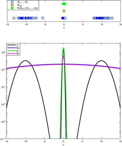
3.6 Example 1 (ctd.)

For the toy example in Section 2 we used the following parameters $$\begin{array}{c}\overline{W}=1,\gamma =0.5,\tau =0.5,N_0=1000,\\ {\omega }_n={(1+M_n/10)}^{-1},Q_0=\mathcal{N}(0,10).\end{array}$$

Figure 1 shows the different states of the chain that, before the first increment takes place, are all sampled from Q₀. The proposed state ${\tilde{X}}_{n+1}$ activates the increment process when the condition $\{W_n({\tilde{X}}_{n+1})>\overline{W}\}$ is satisfied for the first time after the initial phase ($N_0=1000$) is completed. At ${\tilde{X}}_{n+1}$ there is a large discrepancy between the current proposal, Q_n, and the target, ${\pi }_1$. The neighborhood of ${\tilde{X}}_{n+1}$ is identified and defines ${\varphi }_1$, the first component of the incremental mixture.

Fig. 1 (Example 1) Illustration of one AIMM increment for the target π₁. Top: States $X_1,\dots ,X_n$ of the AIMM chain, proposed new state ${\tilde{X}}_{n+1}$ activating the increment process (i.e., satisfying $W_n({\tilde{X}}_{n+1})\ge \overline{W}$), and neighborhood of ${\tilde{X}}_{n+1}$, $\mathfrak{N}({\tilde{X}}_{n+1} | X_1,\dots ,X_n)$. Bottom: Target π₁, defensive kernel Q₀, first increment ${\varphi }_1$, and updated kernel Q₁ plotted on a logarithmic scale.

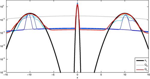
After $n=20,000$ iterations, AIMM has incremented the proposal 15 times. This sequence of proposal distributions can be seen in Figure 2. The first proposals are slightly bumpy and as more samples become available, the proposal distribution gets closer to the target. Thus, even without any information about π₁, AIMM is able to increment its proposal so that the discrepancy between Q_n and ${\pi }_1$ vanishes. This is confirmed by the fact that the acceptance rate edges toward one as the number of components in the mixture increases throughout the algorithm (see Figure 1 in the supplementary materials for an illustration). The AGM-3 proposal density declines to zero in π₁’s low density regions (see Figure 2, bottom panel in supplementary materials), which is an appealing feature in this simple example. However, AGM shrinks its proposal density in locations that have not been visited by the chain. This can be problematic if the sample space is large and it takes time to reasonably explore it (see Section 5).

Fig. 2 (Example 1) Illustration of AIMM sampling from the target π₁ for $n=20,000$ iterations sequence of proposals from Q₀ to Q_n produced by AIMM.

4 Ergodicity of AIMM

4.1 Notation

Let $(\Omega ,\mathcal{A},\mathbb{P})$ be the probability space generated by AIMM. For any event $A\in \mathcal{A},{\mathbb{P}}_A$ denotes the probability measure $\mathbb{P}$ conditionally on A. With some abuse of notations, for any $x\in X,{\mathbb{P}}_x$ refers to the probability measure such that $X_0\sim {\delta }_x$. Let ν and μ be two probability measures defined on $(X,\mathcal{X})$. Recall that the Kullback–Leibler (KL) divergence between ν and μ is defined as $$\mathit{KL}(\nu ,\mu )={\int }_X\hspace{0.17em}\text{log}\hspace{0.17em}\frac{\nu \left(x\right)}{\mu \left(x\right)}\mathrm{d}\nu \left(x\right) .$$

Moreover, the total variation distance between ν and μ can be written as $$\left|\right|\nu -\mu \left|\right|=\underset{A\in \mathcal{X}}{\sup }|\nu (A)-\mu (A\left)\right|=\frac{1}{2}{\int }_X|\mu \left(x\right)-\nu \left(x\right)|\mathrm{d}\rho (x) ,$$ where the latter equality holds if μ and ν are both dominated by a common measure ρ. Finally, for a sequence of random variables ${\left\{X_n\right\}}_{n>0}$, the notations $X_n=o_p(1)$ stands for the convergence of ${\left\{X_n\right\}}_{n>0}$ to zero in probability p (i.e., with respect to the probability measure p), and $X_n=O_p(1)$ means that ${\left\{X_n\right\}}_{n>0}$ is bounded in probability p.

4.2 Ergodicity of Adaptive Markov Chains

In this section, we establish assumptions under which the AIMM process is ergodic, that is, (8) $$\forall x\in X,\hspace{1em}\underset{n\to \infty }{\lim }\left|\right|{\mathbb{P}}_x(X_n\in · )-\pi \left|\right|=0 .$$(8)

We use the theoretical framework developed in Roberts and Rosenthal (2007). In particular, Theorem 2 in Roberts and Rosenthal (2007) states that if the AIMM process satisfies the Diminishing adaptation and Containment conditions (see below) then the process ${\left\{X_n\right\}}_{n>0}$ is ergodic and Equation (8)(8) $$\forall x\in X,\hspace{1em}\underset{n\to \infty }{\lim }\left|\right|{\mathbb{P}}_x(X_n\in · )-\pi \left|\right|=0 .$$(8) holds.

Condition 1. Diminishing adaptation.

For all $x\in X$, the stochastic process $\{{\Delta }_n, n\in \mathbb{N}\}$, defined as (9) $${\Delta }_n:=\underset{x\in X}{\sup }\left|\right|K_{n+1}(x, · )-K_n(x, · )\left|\right|$$(9) converges to zero in ${\mathbb{P}}_x$-probability, that is, ${\Delta }_n=o_{{\mathbb{P}}_x}(1)$.

Condition 2. Containment.

For all $ϵ>0$ and $x\in X$, the stochastic process $\{C_n(ϵ), n\in \mathbb{N}\}$, defined as (10) $$C_n(ϵ):=\inf \{N\in \mathbb{N},|\left|K_n^N\right(X_n, · )-\pi ||<ϵ\}$$(10) is bounded in ${\mathbb{P}}_x$-probability, that is, $C_n(ϵ)=O_{{\mathbb{P}}_x}(1)$.

Even though containment is not a necessary condition for ergodicity (see Fort, Moulines, and Priouret 2011) and in fact seems to hold in most practical situations (see, e.g., Rosenthal 2011), it remains a challenging assumption to establish rigorously for the setup considered in this article, that is, a broad class of target distributions defined on a not necessarily finite or compact state space. In the next section we show that diminishing adaptation holds for the AIMM process described at Section 3, up to minor implementation adjustments, while containment needs to be proven on a case by case basis. We also show that there exists a version of AIMM, conceptually different from the process described at Section 3 that can be made arbitrarily close to it, which is ergodic for any absolutely continuous target distribution π.

4.3 Main Ergodicity Results

We study two variants of AIMM.

4.3.1 Proposal With an Unlimited Number of Increments

The first version of AIMM is similar to the algorithm presented in Section 3. For this version of the algorithm, we prove only that the diminishing adaptation assumption holds under some minor assumptions. Indeed, proving the containment condition is challenging without further assumptions on π, for example, compact support (Craiu, Rosenthal, and Yang 2009) or tail properties (see Bai, Roberts, and Rosenthal (2009) in the context of adaptive random walk Metropolis samplers). Moreover, most proof techniques establishing containment require the space of the adapting parameter to be compact, something which does not hold in this version of AIMM as the number of incremental components can, theoretically, grow to infinity.

Proposition 1.

Assume that there exist three positive constants $(\delta ,\eta ,\lambda )$ such that

A1.The covariance matrix of any component of the mixture satisfies $\det {\Sigma }_k>\delta >0$.

A2.The (unnormalized) incremental mixture weights are defined as

(11) $${\beta }_{M_n+1}=\frac{\eta +\pi {\left({\tilde{X}}_{n+1}\right)}^{\gamma }}{{(1+\eta )}^{M_{n+1}}}\hspace{1em}\text{and}\hspace{1em}{\omega }_n=\frac{1}{1+\sum _{k=1}^{M_n}{\beta }_k}\vee \lambda .$$(11)

A3.The initial kernel Q₀ is subexponential or satisfies $Q_0(x)\propto \hspace{0.17em}\text{exp}\hspace{0.17em}\{\psi (x)\}$ where $\psi =o(x^2)$ $(x\to \infty )$, that is, Q₀ has heavier tail than a Gaussian, for example, multivariate Laplace or t-distribution.

A4.There is a parameter $0<\underset{\_}{W}<\overline{W}$ such that the mixture increments upon the event ${\mathcal{E}}_n\cup {\mathcal{F}}_n$,

$${\mathcal{F}}_n:=\left\{W_n\right({\tilde{X}}_{n+1})<\underset{\_}{W}\}$$

and when it increments upon ${\mathcal{F}}_n$, the new component is equal to Q₀ and the corresponding weight is defined as in Equation (7)(7) $${\beta }_{M_n+1}:\propto \pi {\left({\tilde{X}}_{n+1}\right)}^{\gamma } ,\hspace{1em}\gamma \in (0,1) ,$$(7) .

Then, the AIMM process sampled using conditions A1–A4 satisfies diminishing adaptation, that is, Equation (9)(9) $${\Delta }_n:=\underset{x\in X}{\sup }\left|\right|K_{n+1}(x, · )-K_n(x, · )\left|\right|$$(9) holds.

The proof is given at Section 1 of the supplementary materials.

Remark 1.

Proposition 1 holds for parameters $(\delta ,\eta ,\lambda )$ arbitrarily close to zero. Also, Assumption A1 can be enforced simply by expanding the neighborhood of ${\tilde{X}}_{n+1}$ such that when $\det \text{cov}\{\mathfrak{N}({\tilde{X}}_{n+1})\}<\delta$, $${\Sigma }_{M_n+1}:=\text{cov}\{X_1^{\ast },\dots ,X_k^{\ast }\},$$ where $\{X_1^{\ast },\dots ,X_n^{\ast }\}$ is a permutation of $\{X_1,\dots ,X_n\}$ such that ${\mathrm{D}}_{\mathrm{M}}({\tilde{X}}_{n+1},X_i^{\ast })\le {\mathrm{D}}_{\mathrm{M}}({\tilde{X}}_{n+1},X_{i+1}^{\ast })$ and $k:=\inf \{i\le n, \det \text{cov}(X_1^{\ast },\dots ,X_i^{\ast })\ge \delta \}$.

Remark 2.

The event ${\mathcal{F}}_n$ is the counterpart of ${\mathcal{E}}_n$ and exposes subsets of $X$ where the proposal puts too much probability mass at locations of low π-probability. In this case, the rationale for setting ${\varphi }_{M_n+1}=Q_0$ is to reduce the probability mass of the proposal locally by increasing the weight associated to the initial proposal Q₀, assumed to be vague.

4.3.2 Proposal With Adaptation on a Compact Set

The second version of AIMM that we study here represents somewhat a slight conceptual departure from the original algorithm presented in Section 3. We stress that the assumptions A1–A4 from Section 4.3.1 are not required here.

Proposition 2.

Assume that:

B1.The AIMM process $\{X_n, n\in \mathbb{N}\}$ has bounded jumps, that is, there exists D > 0 such that for all $n\in \mathbb{N}$

(12) $$\mathbb{P}\left\{\right||X_n-X_{n+1}||\le D\}=1 .$$(12)

B2.There is a compact set $\mathcal{K}\subset X$ such that the weight ${\left\{{\omega }_n\right\}}_n$ in the proposal (4) is replaced by ${\left\{{\overline{\omega }}_n^{\mathcal{K}}\right\}}_n$ (13) $${\overline{\omega }}_n^{\mathcal{K}}={\omega }_n\vee 1_{X_n\notin \mathcal{K}} ,$$(13) that is, if the process is such that $X_n\notin \mathcal{K}$ then the proposed state is generated from Q₀ with probability one. Conversely, if the process is such that $X_n\in \mathcal{K}$, then the proposed state is generated as explained in Section 3, that is, from Q_n (4). We denote this proposal by ${\overline{Q}}_n^{\mathcal{K}}$.

B3.The number of incremental components in the adaptive proposal is capped, that is, there is a finite $M\in \mathbb{N}$ such that $\mathbb{P}(M_n\le M)=1$ and the mean μ_n and covariance Σ_n of each component are defined on a compact space.

If the AIMM process presented in Section 3 satisfies B1–B3, then it is ergodic.

This result is a consequence of Theorem 2 of Roberts and Rosenthal (2007) combined with the recent developments in Craiu et al. (2015) and Rosenthal and Yang (2017). The proof is given at Section 2 of the supplementary materials.

We now explain how, in practice, a version of AIMM compatible with the assumptions of Proposition 2 can be constructed and made arbitrarily close to the version of AIMM presented in Section 3. First, fix an arbitratrily large constant $D<\infty$. Assumption B1 holds by construction if ${\tilde{X}}_{n+1}\sim {\overline{Q}}_n^{\mathcal{K}}$ is automatically rejected when $\left|\right|{\tilde{X}}_{n+1}-X_n\left|\right|>D$. Assumption B2 holds by construction if ${\overline{Q}}_n^{\mathcal{K}}$ is used instead of Q_n in the AIMM algorithm presented in Section 3. Finally, Assumption B3 is satisfied by slightly modifying the adaptation mechanism proposed in Section 3. Define two arbitrarily large constants L > 0 and $M\in \mathbb{N}$ and increment the proposal upon the event ${\overline{\mathcal{E}}}_n:={\mathcal{E}}_n\cap \{M_n<M\}$ and in the following way $${\overline{\mu }}_{M_n+1}:={\tilde{X}}_{n+1}{|}_L ,\hspace{1em}{\overline{\Sigma }}_{M_n+1}:=\text{cov}\left\{{\overline{\mathfrak{N}}}_L\right({\tilde{X}}_{n+1} | X_1,\dots ,X_n)\} ,$$ where for any vector $x\in {\mathbb{R}}^d$ and any L > 0 $$\begin{array}{c}x{|}_L=\left\{\right\{x_1\wedge L\}\vee -L,\dots ,\{x_d\wedge L\}\vee -L\}\hspace{1em}\text{and}\\ {\overline{\mathfrak{N}}}_L=\left\{X_i{|}_L,X_i\in \mathfrak{N}({\tilde{X}}_{n+1} | X_1,\dots ,X_n)\right\} .\end{array}$$

The definition of the unnormalized weight ${\beta }_{M_n+1}$ (Equation (7)(7) $${\beta }_{M_n+1}:\propto \pi {\left({\tilde{X}}_{n+1}\right)}^{\gamma } ,\hspace{1em}\gamma \in (0,1) ,$$(7) ) is unchanged.

5 Simulations

In this section, we consider three target distributions:

• ${\pi }_2$, the banana shape distribution used in Haario, Saksman, and Tamminen (2001);

• ${\pi }_3$, the ridge like distribution used in Raftery and Bao (2010);

• ${\pi }_4$, the bimodal distribution used in Raftery and Bao (2010).

Each of these distributions has a specific feature, resulting in a diverse set of challenging targets: ${\pi }_2$ is heavy tailed, ${\pi }_3$ has a narrow, nonlinear and ridge-like support, and ${\pi }_4$ has two distant modes. We consider ${\pi }_2$ and ${\pi }_4$ in different dimensions: $d\in \{2,10,40\}$ for ${\pi }_2$ and $d\in \{4,10\}$ for ${\pi }_4$. We compare AIMM (Algorithm 1) with several other algorithms that are briefly described along with some performance indicators that are also outlined at Section 3 of the supplementary materials. We used the following default parameters for AIMM $$\gamma =0.5 ,\hspace{1em}\tau =0.5 ,\hspace{1em}\kappa =0.1 ,\hspace{1em}{N}_0=1000\sqrt{d} .$$

The parameter requiring the most careful design is $\overline{W}$. A poor choice of $\overline{W}$ may result in a proposal that never increments or that increments too often. For each scenario, we implemented AIMM with different thresholds $\overline{W}$ valued around d to monitor the tradeoff between adaptation and computational efficiency of the algorithm. In our experience, the choice $\overline{W}=d$ has worked reasonably well in a wide range of examples, but there is no theoretical guarantee supporting this choice which is not optimal in any sense. Intuitively, as the dimension of the state space increases a higher threshold is required, too many kernels being created otherwise. However, a satisfactory choice of $\overline{W}$ may vary depending on the target distribution and the available computational budget. It is also possible to adapt $\overline{W}$ online during an initial phase of the algorithm as the theory remains valid as long as $\overline{W}$ is eventually set constant. Two particular situations where an automated choice of $\overline{W}$ may be particularly beneficial include setups where Q₀ and π yield a significant mismatch and where π is known up to a normalizing constant. In the first case, it is necessary to initialize $\overline{W}$ at a small value and gradually increasing it until reaching the desired value. In the second one, the threshold $\overline{W}$ is adapted at the beginning of the algorithm to get the incremental process started. The threshold adaptation produces a sequence of thresholds ${\left\{{\overline{W}}_n\right\}}_n$ such that $Q_n\{W_n(X)>{\overline{W}}_n\}\approx u_n$ where u_n is a decreasing sequence with $u_n\to 0$ such as $u_n={10}^{-3}{n}^{-0.2}$. Since sampling from Q_n (a mixture of Gaussian distributions), can be performed routinely, ${\overline{W}}_n$ is derived from a Monte Carlo estimation. As little precision is required, the Monte Carlo approximation should be rough to limit the computational burden generated by the threshold adaptation. Also, those samples used to set ${\overline{W}}_n$ can be recycled and serve as proposal states for the AIMM chain so that this automated threshold mechanism comes for free.

5.1 Banana-Shaped Target Distribution

Example 2.

Let $X={\mathbb{R}}^d,{\pi }_2(x)={\Psi }_d(f_b(x);m,S)$ where ${\Psi }_d( · ; m,S)$ is the d-dimensional Gaussian density with mean m and covariance matrix S, and let $f_b:{\mathbb{R}}^d\to {\mathbb{R}}^d$ be the mapping defined, for any $b\in \mathbb{R}$, by $$f_b:\left(\begin{array}{c}{x}_1\\ x_2\\ x_3\\ ⋮\\ x_d\end{array}\right)\to \left(\begin{array}{c}{x}_1\\ x_2+b x_1^2-100b\\ x_3\\ ⋮\\ x_d\end{array}\right) .$$

We consider ${\pi }_2$ in dimensions d = 2, d = 10, and d = 40 and refer to the marginal of ${\pi }_2$ in the ith dimension as ${\pi }_2^{(i)}$. The parameters $m=0_d$ and $S=\text{diag}([100,1_{d-1}])$ are held constant. The target is banana-shaped along the first two dimensions, and is challenging since the high density region has a thin and wide ridge-like shape with narrow but heavy tails. Unless otherwise stated, we use b = 0.1 which accentuates these challenging features of ${\pi }_2$. We first use the banana-shaped target ${\pi }_2$ in dimension d = 2 to study the influence of AIMM’s user-defined parameters on the sampling efficiency.

5.1.1 Influence of the Defensive Distribution

With limited prior knowledge of $\pi$, choosing Q₀ can be challenging. Here we consider three defensive distributions Q₀, represented by the black dashed contours in Figure 3. The first two are Gaussian, respectively, located close to the mode and in a nearly zero probability area and the last one is the uniform distribution on the set $\mathfrak{S}=\{x\in X ,x_1\in (-50,50),x_2\in (-100,20)\}$. Table 2 and Figure 3 show that AIMM is robust with respect to the choice of Q₀. Even when Q₀ yields a significant mismatch with ${\pi }_2$ (second case), the incremental mixture reaches high density areas, progressively uncovering higher density regions. The price to pay for a poorly chosen Q₀ is that more components are needed in the incremental mixture to match ${\pi }_2$, as shown by Table 2. The other statistics reported in Table 2 are reasonably similar for the three choices of Q₀.

Fig. 3 (Example 2: π₂ target, d = 2) Incremental mixture created by AIMM for three different initial proposals. Top row: Q₀ is a Gaussian density (the region inside the black dashed ellipses contains 75% of the Gaussian mass) centred on a high density region (left) and a low density region (right). Bottom row: Q₀ is Uniform (with support corresponding to the black dashed rectangle). The components ${\varphi }_1,\dots ,{\varphi }_{M_n}$ of the incremental mixture obtained after $n=100,000$ MCMC iterations are represented through (the region inside the ellipses contains 75% of each Gaussian mass). The color of each ellipse illustrates the corresponding component’s relative weight ${\beta }_{\ell }$ (from dark blue for lower weights to red).

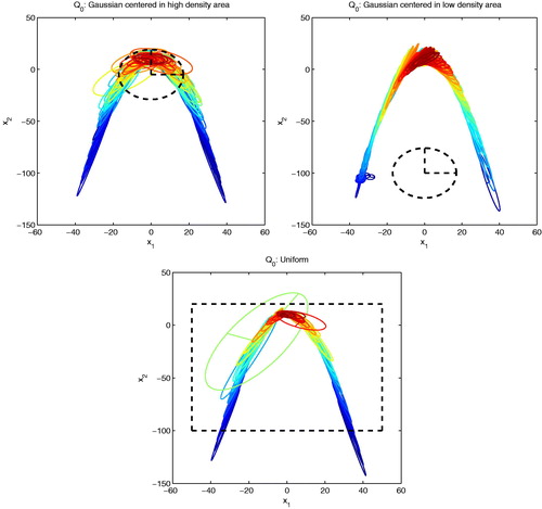
Table 2 (Example 2: π₂ target, d = 2) Influence of the initial proposal Q₀ on AIMM outcome after $n=100,000$ MCMC iterations (replicated 20 times).

Q0	Mn	$\mathit{ESS}$	$\mathit{ACC}$	$\mathit{KL}$	$\mathit{JMP}$	$\mathit{EFF}$ ($\times {10}^{-4}$)
Gaussian on a high density region	41	0.19	0.35	0.59	197	11
Gaussian on a low density region	157	0.23	0.37	0.71	245	4
Uniform on $\mathfrak{S}$	39	0.24	0.38	0.62	320	11

NOTE: M_n is the number of components created by AIMM, $\mathit{ESS}$ is the effective sample size, $\mathit{ACC}$ is the acceptance rate, $\mathit{KL}$ is the KL divergence between ${\pi }_2$ and the chain distribution, $\mathit{JMP}$ is the average distance between two consecutive states of the chain, and $\mathit{EFF}$ is a time-normalized ESS.

5.1.2 Influence of the Threshold

Even though we recommend the default setting $\overline{W}=d$, we analyze the performances of AIMM for different values of $\overline{W}$. We consider the same setup as in the previous subsection with the uniform defensive distribution Q₀ and report the outcome of the AIMM algorithm in Table 3a. As expected, the lower the threshold $\overline{W}$, the larger the number of kernels and the better is the mixing. In all cases, the adaptive transition kernel eventually stabilizes (faster if $\overline{W}$ is large), as illustrated by Figure 4(a), resulting from the fact that the event ${\mathcal{E}}_n=\{W_n({\tilde{X}}_{n+1})>\overline{W} ,{\tilde{X}}_{n+1}\sim Q_n\}$ occurs less often as n increases. As $\overline{W}$ decreases, the KL divergence between ${\pi }_2$ and the chain reduces while the CPU cost increases since more components are created. Therefore, the sampling efficiency is best for an intermediate threshold such as $\text{log}\hspace{0.17em}\overline{W}=.75$. Finally, when the threshold is too low, the distribution of the chain converges more slowly to ${\pi }_2$; see, for example, Table 3(a) where the $\mathit{KL}$ indicator (defined as the KL divergence between ${\pi }_2$ and the sample path of the AIMM chain; see supplementary materials) is larger for $\text{log}\hspace{0.17em}\overline{W}=0.25$ than for $\text{log}\hspace{0.17em}\overline{W}=0.5$. Indeed when $\overline{W}\ll 1$, too many components are created to support high density areas and this slows down the exploration process of the lower density regions.

Fig. 4 (Example 2: π₂ target, d = 2) AIMM’s incremental mixture design after $n=100,000$ MCMC iterations. (a) Evolution of the number of kernels M_n created by AIMM for different thresholds. (b) Evolution of the KL divergence between ${\pi }_2$ and the incremental proposal Q_n, plotted in lin-log scale.

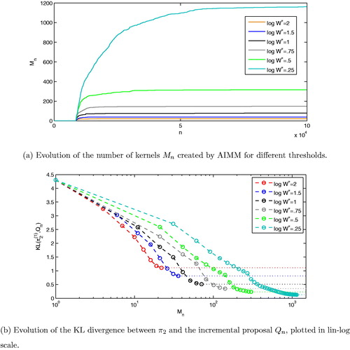
Table 3 (Example 2: π₂ target, d = 2) Influence of the threshold $\overline{W}$ on AIMM and f-AIMM outcomes after $n=100,000$ MCMC iterations (replicated 20 times).

(a) AIMM
$\text{log}\hspace{0.17em}\overline{W}$	Mn	$\mathit{ESS}$	$\mathit{ACC}$	$\mathit{KL}$	$\mathit{JMP}$	$\mathit{CPU}$	$\mathit{EFF}$ $(\times {10}^{-4})$
10	0	0.03	0.01	14.06	10	45	2
2	21	0.16	0.27	0.72	169	154	10
1.5	39	0.24	0.38	0.62	235	245	10
1	79	0.37	0.53	0.54	331	330	12
0.75	149	0.48	0.64	0.53	286	658	7
0.5	317	0.64	0.75	0.51	451	2199	3
0.25	1162	0.71	0.87	0.54	505	6201	1
(b) f-AIMM
$\text{log}\hspace{0.17em}\overline{W}$	$M_{\text{max}}$	$\mathit{ESS}$	$\mathit{ACC}$	$\mathit{KL}$	$\mathit{JMP}$	$\mathit{CPU}$	$\mathit{EFF}$ $(\times {10}^{-4})$
1.5	25	0.29	0.51	0.59	268	255	11
0.75	100	0.53	0.69	0.53	409	421	13
0.5	200	0.67	0.80	0.51	474	1151	6

5.1.3 Speeding up AIMM

The computational efficiency of AIMM depends, to a large extent, on the number of components added in the proposal distribution, M_n. For this reason we consider a slight modification of the original AIMM algorithm to limit the number of possible components, thereby improving the computational speed of the algorithm. This variant of the algorithm is referred to as fast AIMM (denoted by f-AIMM) and proceeds as follows: let $M_{\text{max}}$ be the maximal number of components allowed in the incremental mixture proposal. If $M_n>M_{\text{max}}$, only the last $M_{\text{max}}$ added components are retained, in a moving window fashion. This truncation has two main advantages, (i) approximately linearizing the computational burden once $M_{\text{max}}$ is reached, and (ii) forgetting the first, often transient components used to jump to high density areas (see, e.g., the loose ellipses in Figure 3, especially the very visible ones in the bottom panel).

Table 3 shows that f-AIMM outperforms the original AIMM, with some setups being nearly twice as efficient; compare, for example, AIMM and f-AIMM with $\text{log}\hspace{0.17em}\overline{W}=0.5$ in terms of efficiency (last column). Beyond efficiency, comparing $\mathit{KL}$ for a given number of mixture components (M_n), shows that ${\pi }_2$ is more quickly explored by f-AIMM than by AIMM. Numerical comparisons on this example of f-AIMM with other samplers (AMH, RWMH, AGM, IM) are reported in Section 5.1 of the supplementary materials. AIMM seems to yield the best tradeoff between convergence and variance in all dimensions. Inevitably, as d increases, ESS shrinks and KL increases for all algorithms but AIMM still maintains a competitive advantage over the other approaches. The other four algorithms struggle to visit the tail of the distribution. Thus, AIMM is doing better than (i) the nonindependent samplers (RWMH and AMH) that manage to explore the tail of a target distribution but need a large number of transitions to return there, and (ii) the independence samplers (IM and AGM) that can quickly explore different areas but fail to venture into the lower density regions. An animation corresponding to the exploration of π₂ in dimension 2 by AIMM, AGM, and AMH can be found at http://mathsci.ucd.ie/∼fmaire/AIMM/banana.html.

5.2 Ridge Like Example

Example 3.

Let $X={\mathbb{R}}^6$ and ${\pi }_3(x)\propto {\Psi }_6(x;{\mu }_i,{\Gamma }_i){\Psi }_4(g(x);{\mu }_o,{\Gamma }_o)$, where ${\Psi }_d( · ; m,S)$ is the d-dimensional Gaussian density with mean m and covariance matrix S. The target parameters $({\mu }_i,{\mu }_o)\in {\mathbb{R}}^6\times {\mathbb{R}}^4$ and $({\Gamma }_i,{\Gamma }_o)\in {\mathcal{M}}_6(\mathbb{R})\times {\mathcal{M}}_4(\mathbb{R})$ are, respectively, known means and covariance matrices and g is a nonlinear deterministic mapping ${\mathbb{R}}^6\to {\mathbb{R}}^4$ defined as $$g(x_1,\dots ,x_6)=\{\begin{array}{c}\prod _{i=1}^6{x}_i ,\hfill \\ x_2{x}_4 ,\hfill \\ x_1/x_5 ,\hfill \\ x_3{x}_6 .\hfill \end{array}$$

In this context, ${\Psi }_6( · ;{\mu }_i,{\Gamma }_i)$ can be regarded as a prior distribution and ${\Psi }_4( · ;{\mu }_o,{\Gamma }_o)$ as a likelihood, the observations being some functional of the hidden parameter $x\in {\mathbb{R}}^6$.

Such a target distribution often arises in physics. Similar target distributions often arise in Bayesian inference for deterministic mechanistic models and in other areas of science, engineering and environmental sciences (see, e.g., Poole and Raftery 2000; Bates, Cullen, and Raftery 2003). They are hard to sample from because the probability mass is concentrated around thin curved manifolds. We compare f-AIMM with RWMH, AMH, AGM, and IM first in terms of their mixing properties; see Table 4. We also ensure that the different methods agree on the mass localization by plotting a pairwise marginal; see Figure 5 of the supplementary materials. In this example, f-AIMM clearly outperforms the four other methods in terms of both convergence and variance statistics. In fact, we observe in the same figure that f-AIMM is the only sampler able to discover a secondary mode in the marginal distribution of the second and fourth target components (X₂, X₄).

Fig. 5 (Example 5) Information regarding the acceptance rate of 100 AIMM runs are reported on the left panel and the evolution of the number of components for about 10 runs throughout the sampling is shown on the right panel.

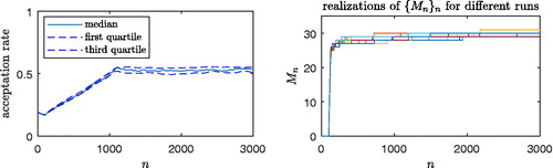
Table 4 (Example 3: π₃ target, d = 6) Comparison of f-AIMM with the four other samplers after $n=200,000$ iterations (replicated 10 times).

	$\overline{W}$	$M_{\text{max}}$	$\mathit{ACC}$	$\mathit{ESS}$	$\mathit{CPU}$	$\mathit{EFF}$	$\mathit{JMP}$
f-AIMM	10	20	0.049	0.015	274	$5.2\times {10}^{-5}$	0.08
f-AIMM	1	70	0.169	0.089	517	$1.7\times {10}^{-4}$	0.27
f-AIMM	0.1	110	0.251	0.156	818	$1.9\times {10}^{-4}$	0.38
RWMH		–	0.23	0.001	109	$9.2\times {10}^{-6}$	0.007
AMH		–	0.42	0.002	2105	$9.5\times {10}^{-7}$	0.004
AGM-MH		100	0.009	0.002	2660	$3.4\times {10}^{-6}$	0.003
IM		–	0.003	0.001	199	$5.5\times {10}^{-6}$	0.003

5.3 Bimodal Distribution

Example 4.

In this example, ${\pi }_4$ is a posterior distribution defined on the state space $X={\mathbb{R}}^d$, where $d\in \{4,10\}$. The likelihood is a mixture of two d-dimensional Gaussian distributions with weight $\lambda =0.5$, mean and covariance matrix as follows $$\begin{array}{c}{\mu }_1=0_{\mathrm{d}} ,\hspace{1em}{\Sigma }_1={\text{AR}}_{\mathrm{d}}(-.95) ,\\ {\mu }_2=9_{\mathrm{d}} ,\hspace{1em}{\Sigma }_2={\text{AR}}_{\mathrm{d}}\left(.95\right) ,\end{array}$$

where for all $\rho >0,{\text{AR}}_{\mathrm{d}}(\rho )$ is the d-dimensional first-order autoregressive matrix whose coefficients are $$\text{for}1\le (i,j)\le d ,\hspace{1em}{m}_{i,j}(\rho )={\rho }^{\max (i,j)-1} .$$

The prior is the uniform distribution $\mathcal{U}({[-3,12]}^d)$. For f-AIMM and IM, Q₀ is set as this prior distribution, while for AGM, the centers of the Gaussian components in the initial proposal kernel are drawn according to the same uniform distribution. For AMH, the initial covariance matrix ${\Sigma }_0$ is set to be the identity matrix.

Several plots showing the outcome of this experiment are presented in Section 5.3 of the supplementary materials. On the one hand, in both setups $M_{\text{max}}=100$ and $M_{\text{max}}=200$, f-AIMM is more efficient at discovering and jumping from one mode to the other and allowing more kernels in the incremental mixture proposal will result in faster convergence. On the other hand, because of the distance between the two modes, RWMH visits only one while AMH visits both but in an unbalanced fashion. Increasing the dimension from d = 4 to d = 10 makes AMH unable to visit the two modes after $n=200,000$ iterations. As for AGM, the isolated samples reflect a failure to explore the state space. These facts are confirmed in Table 5 which highlights the better mixing efficiency of f-AIMM relative to the four other algorithms and in Table 6 which shows that f-AIMM is the only method which, after $n=200,000$ iterations, visits the two modes with the correct proportion.

Table 5 (Example 4: π₄ target, $d\in \{4,10\}$) Comparison of f-AIMM with RWMH, AMH, AGM, and IM after $n=200,000$ iterations (replicated 100 times).

(a) π4 in dimension d = 4
	$\overline{W}$	$M_{\text{max}}$	$\mathit{ACC}$	$\mathit{ESS}$	$\mathit{CPU}$	$\mathit{EFF}$	$\mathit{JMP}$
f-AIMM	5	100	0.69	0.30	408	$7.3\times {10}^{-4}$	68
RWMH		–	0.23	$3.1\times {10}^{-3}$	93	$3.4\times {10}^{-5}$	0.09
AMH		–	0.26	$2.7\times {10}^{-2}$	269	$1.0\times {10}^{-4}$	0.64
AGM-MH		100	$3.0\times {10}^{-3}$	$5.0\times {10}^{-4}$	3517	$1.4\times {10}^{-7}$	0.29
IM		–	$3.3\times {10}^{-4}$	$5.9\times {10}^{-4}$	81	$7.3\times {10}^{-6}$	0.05
(b) π4 in dimension d = 10
	$\overline{W}$	$M_{\text{max}}$	$\mathit{ACC}$	$\mathit{ESS}$	$\mathit{CPU}$	$\mathit{EFF}$	$\mathit{JMP}$
f-AIMM	20	100	0.45	0.18	1232	$1.4\times {10}^{-4}$	116.4
f-AIMM	10	200	0.64	0.25	1550	$1.6\times {10}^{-4}$	200.1
RWMH		–	0.38	$7.2\times {10}^{-4}$	476	$1.7\times {10}^{-6}$	0.07
AMH		–	0.18	$1.3\times {10}^{-3}$	2601	$5.0\times {10}^{-7}$	0.57
AGM-MH		100	$2.6\times {10}^{-4}$	$5.0\times {10}^{-4}$	4459	$1.1\times {10}^{-7}$	$7.1\times {10}^{-3}$
IM		–	$6.4\times {10}^{-5}$	$6.1\times {10}^{-4}$	473	$1.2\times {10}^{-6}$	$4.1\times {10}^{-3}$

Table 6 (Example 4: π₄ target, $d\in \{4,10\}$) Mean square error (MSE) of the mixture parameter λ, for the different algorithms (replicated 100 times).

	$\overline{W}$	$M_{\text{max}}$	$\mathit{MSE}(\lambda ),d=4$	MSE($\lambda$), d = 10
f-AIMM	5	100	0.0001	0.06
f-AIMM	20	100	0.0006	0.09
f-AIMM	10	200	0.0024	0.01
RWMH		–	0.25	0.25
AMH		–	0.15	0.25
AGM-MH		100	0.22	0.25
IM		–	0.03	0.20

6 Applications

The statistical analysis of two real data problems is carried out:

• the inference of a semiparametric regression model applied to the Boston Housing dataset (available at www.cs.utoronto.ca/∼delve/data/boston). This model has also been studied in Smith and Kohn (1996) and more recently, using an AGM MCMC method in Giordani and Kohn (2010). This model has seven parameters.

• the inference of a Bayesian hierarchical model related to the James–Stein estimator (James and Stein 1961) applied to batting averages of 18 MLB players (first column of Table 1 in Efron and Morris (1975)). This model has also been used to validate the adaptation of an adaptive MCMC algorithm proposed in Roberts and Rosenthal (2009). This model has twenty parameters.

6.1 Semiparametric Regression

Example 5.

We consider the following semiparametric regression model $$Y_i=\gamma Z_i+\sum _{\ell =1}^H{f}_{\ell }\left(X_{\ell ,i}\right)+{\sigma }_{ϵ}{\zeta }_i ,\hspace{1em}{\zeta }_i\sim \mathcal{N}(0,1) ,$$ where γ is the regression vector, Z_i are the covariates for observation Y_i, $f_1,\dots ,f_H$ are nonparametric regression functions (quadratic polynomial splines) and for all $\ell \le H,X_{\ell ,i}\in Z_i$ is a critical covariate whose impact on the dependent variable is not sufficiently well described by the parametric term and thus requires an additional nonparametric regression term for further flexibility. Considering a Bayesian analysis of this model, a Gaussian prior distribution is assigned to γ and to the parameters ${\beta }_1,\dots ,{\beta }_H$ controlling the H splines. An inverse gamma prior is prescribed to the additive noise parameter ${\sigma }_{ϵ}$. It is difficult to choose the β’s priors variance and the inference is quite sensitive to this issue (see Smith and Kohn 1996; Giordani and Kohn 2010). As a consequence the variances ${\tau }_1,{\tau }_2,\dots ,{\tau }_H$ are included in the model and a log-normal hyperprior is assigned to those parameters. Since the regression parameters $(\gamma ,{\beta }_1,\dots ,{\beta }_H)$ are conjugated given the variances $\theta :=({\tau }_{ϵ},{\tau }_1,\dots ,{\tau }_H)$ sampling from the posterior of the model can be done by (i) sampling $\theta \sim \mathrm{Pr}( · | Y)$ and (ii) sampling $(\gamma ,{\beta }_1,\dots ,{\beta }_H)\sim \mathrm{Pr}( · | Y,\theta )$. The marginal posterior of θ cannot be sampled using direct methods but since its analytical expression is known up to a normalizing constant, one can be used MCMC to perform (i). In this example, the data are the logarithm of the median market value of owner-occupied home for the Boston metropolitan area reported in Harrison and Rubinfeld (1978). It contains 506 observations, 13 covariates H = 6 of which beneficiate from an additional nonparametric description. The dimension of the parameter of interest θ is thus d = 7 and to avoid sampling in a constrained space, we use AIMM to sample $\text{log}\hspace{0.17em}\theta$ given $Y_1,\dots ,Y_{506}$.

We follow the notations and the setup proposed in Giordani and Kohn (2010) where further details can be found, with two exceptions. First, using 30 knots for each spline in the nonparametric part of the model (as recommended in Giordani and Kohn (2010)) made the unnormalized posterior $\pi (\mathrm{d}\theta | Y)$ quite instable: the likelihood $y|\theta$ is a normal whose covariance matrix is nearly singular for a large range of plausible parameters (a fact which was already noted in Smith and Kohn (1996, sec. 6.2)). We thus used only 10 control points per spline, which is closer to what is recommended in Smith and Kohn (1996) and alleviates this numerical problem. Finally, we have set the variance of the parametric regression term to $v_{\gamma }^2=10$, this parameter is not specified in the analysis of Giordani and Kohn (2010).

6.1.1 Results

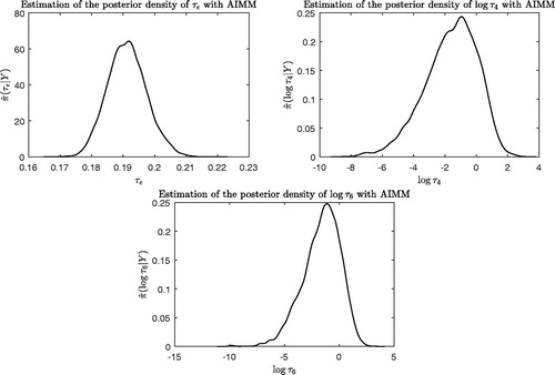
In the experimental setup considered, AIMM ended up incrementing about 30 times on average so that when M_n stabilizes AIMM acceptance rate is around 55%, as shown in Figure 5. Figure 6 reports the estimated posterior distribution of three parameters after a long AIMM run. We note that the inference carried out is similar to what was obtained in the study of this dataset using AGM carried out in Giordani and Kohn (2010). In particular, we find that most variance parameters are log-normally distributed a posteriori, except for two parameter related to the covariates X₄ and X₆ which matches the analysis of Giordani and Kohn (2010). We note however that the additive noise SD posterior distribution is slightly shifted compared to the result of these authors, probably because the prior distribution of this parameter is different in our implementation. We observe that the acceptance rate of AIMM is “penalized” by the conservative choice of ω_n. Indeed, with about $M_n\approx 30$ kernels in the mixture, we have ${\omega }_n\approx 1/4$ which means that, approximately, at every four AIMM transition the proposed state is drawn from Q₀ which is, in this example, very uninformative: this shows that the quality of the AIMM adaptation is similar to, if not better than AGM in this example. Finally, we mention that the adaptive random walk Metropolis algorithm (Haario, Saksman, and Tamminen 2001) was implemented in this example but the results were not relevant: after the initial nonadaptive phase, the estimated covariance matrix quickly deteriorates and the chain remains stuck for long period of times.

Fig. 6 (Example 5) Marginal posterior distribution of three parameters of the model estimated after 70,000 iterations of AIMM.

6.2 Empirical Bayes and the James–Stein Estimator

Example 6.

We consider the following hierarchical model with $i\in \{1,\dots ,K\}$ (14) $$\left(\mathrm{i}\right){\vartheta }_i\sim \mathcal{N}(\mu ,A),\hspace{1em}\left(\text{ii}\right)Y_i\sim \mathcal{N}({\vartheta }_i,V) .$$(14)

The parameters of interest consist in $\theta :=(\hspace{0.17em}\text{log}\hspace{0.17em}A,\mu ,{\vartheta }_1,\dots ,{\vartheta }_K)$, while the matrix V is set to the empirical Bayes estimator of the observed data $Y_1,\dots ,Y_K$. The case $Y_i\in \mathbb{R}$ is considered so that θ is defined on a K + 2 dimensional state space. We proceed to the Bayesian inference of θ given $Y_1,\dots ,Y_K$ and thus assign an inverse gamma prior to A and a normal prior to μ. This model is of particular interest since it corresponds to the Bayesian formulation of the James–Stein estimator (James and Stein 1961): indeed the posterior mean of θ in the hierarchical model Equation (14)(14) $$\left(\mathrm{i}\right){\vartheta }_i\sim \mathcal{N}(\mu ,A),\hspace{1em}\left(\text{ii}\right)Y_i\sim \mathcal{N}({\vartheta }_i,V) .$$(14) defines a general class of empirical Bayes estimators which includes the James–Stein estimator, see Efron and Morris (1975) and Rosenthal (1996) for more details. In this example, the data are the 1970 batting average for 18 Baseball players (see Table 1 of Efron and Morris (1975)) and θ is thus a 20-dimensional parameters. The hyperpriors were chosen as in Roberts and Rosenthal (2009).

6.2.1 Results

Figure 7 reports some marginal posterior distributions estimated by AIMM and ARMS. Clearly, ARMS has not totally converged at that point as some probability mass is missing in the tails of each marginal. This may explain why ARMS seems to be slightly better in terms of acceptance rate and integrated autocorrelation time than AIMM as shown in Table 7. Indeed, an independent proposal that does not dominate the tail of a distribution correctly usually yields a misleading high acceptance rate as the risky moves are simply not attempted. We also include the results for the regional adaptive Metropolis algorithm (RAMA) reported from Roberts and Rosenthal (2009). We note that comparing adaptive independent MCMC and adaptive random walk MCMC is perhaps not very informative as they are structurally different and Table 7 does not probably give a fair assessment of RAMA since (i) the proposal density is adapted so that the sampler acceptance rate is 0.23 and (ii) the average squared jumping distance is always smaller of several order of magnitude (especially in high-dimensional settings) for random walks than for independent proposal algorithms.

Fig. 7 (Example 6) Marginal posterior of four parameters estimated by AIMM and ARMS after a long run of 100,000 iterations of both algorithm (full swipe update Metropolis-within-Gibbs for ARMS).

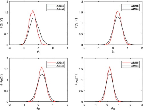
Table 7 (Example 6) Comparison of the performance of three adaptive MCMC samplers: acceptance rate, integrated autocorrelation time and average squared jumping distance.

	Acc rate	IACT	Avg sq. distance ($\times {10}^{-4}$)
AIMM	0.49	1.12	16,203
ARMS	0.53	0.98	11,270
RAMA	0.23	31.6	2.756

NOTE: Results for AIMM and ARMS are estimated based after 10,000 iterations of 100 independent runs (full swipe update Metropolis-within-Gibbs for ARMS). Results for RAMA were reported from (Roberts and Rosenthal 2009, Table p. 360).

7 Discussion

Although implicitly evaluated in an (nonadaptive) independence Metropolis–Hastings transition, the information conveyed by the ratio of importance weights is lost because of the threshold set to one in the MH acceptance probability. Indeed, while at X_n and given two realizations of the proposal Q, say ${\tilde{X}}_{n+1}$ and ${\tilde{Y}}_{n+1}$, the two events $\{W({\tilde{X}}_{n+1})>W(X_n)\}$ and $\{W({\tilde{Y}}_{n+1})\gg W(X_n)\}$ result in the same transition, that is, the proposed move is accepted with probability one, regardless of the magnitude difference between $W({\tilde{X}}_{n+1})/W(X_n)$ and $W({\tilde{Y}}_{n+1})/W(X_n)$. This article aims to design an adaptive MCMC algorithm that makes use of this information by incrementing the independence MH proposal distribution in the latter case and not in the former.

The general methodology, referred to as AIMM, presented and studied in this article is a novel adaptive MCMC method to sample from challenging distributions. Theoretically, we establish under very mild assumptions, that if it only adapts on a compact set and has bounded jumps, this algorithm generates an ergodic process for any distribution of interest known up to a normalizing constant. We show that these conditions can always be enforced by using a specific implementation. In simpler implementations where those conditions may not be verified, the algorithm is nevertheless shown to work well in practice. We provide an even more efficient algorithm, referred to as f-AIMM, that guarantees that the incremental proposal evaluation does not slow down the algorithm. This algorithm can be seen as a series of AIMM algorithms where Gaussian components are progressively dropped. As a consequence, f-AIMM is compatible with the theoretical framework developed at Section 4. In particular, provided that it only adapts on a compact set and has bounded jumps, this algorithm is invariant for any target distribution. We illustrate its performance in a variety of challenging sampling scenarios.

Compared to other existing adaptive MCMC methods, AIMM needs less prior knowledge of the target. Its strategy of incrementing an initial naive proposal distribution with Gaussian kernels leads to a fully adaptive exploration of the state space. Conversely, we have shown that in some examples the adaptiveness of some other MCMC samplers may be compromised when an unwise choice of parametric family for the proposal kernel is made. The performance of AIMM depends strongly on the threshold $\overline{W}$ which controls the adaptation rate. This parameter should also be set according to the computational budget available. When the normalizing constant of π is unknown or when $X$ is high-dimensional, we recommend opting for an automated adaptation of $\overline{W}$ (such as the scheme described at the beginning of Section 5) that allows to increment regularly the proposal kernel. Again, we stress that this work is pioneering the use of semiparametric adaptive kernels and does not consist in an exhaustive study of this algorithm: a reader may see our research as a basis for further optimization and may find more efficient ways to choose AIMM parameters according to their problem at hand. However, we stress that two aspects of the AIMM’s adaptation are essential: first, the defensive kernel is crucial as it safeguards the possibility to discover new parts of the support of π at a later stage of the sampling and its weight in the mixture ω_n should thus not decrease too fast. Second, if an automated choice of $\overline{W}$ is used, the adaptation scheme must eventually lead to a constant threshold.

The adaptive design of AIMM was inspired by incremental mixture importance sampling (IMIS) (Raftery and Bao 2010). IMIS iteratively samples and weights particles according to a sequence of importance distributions that adapt over time. The adaptation strategy is similar to that in AIMM: given a population of weighted particles, the next batch of particles is simulated by a Gaussian kernel centered at the particle having the largest importance weight. However, IMIS and AIMM are structurally different since the former is an adaptive importance sampling method while the latter is an adaptive MCMC algorithm. Comparing them on a fair basis is difficult. In particular, the ESS estimators for the two methods stem from different approximations. The computational efficiency of IMIS suffers from the fact that, at each iteration, the whole population of particles must be reweighted to maintain the consistency of the importance sampling estimator. By contrast, at each transition, AIMM evaluates only the importance weight of the new proposed state. However, since IMIS calculates the importance weight of large batches of particles, it acquires a knowledge of the state space more quickly than AIMM which accepts/rejects one particle at a time.

We therefore expect AIMM to be more efficient in situations where the exploration of the state space requires a large number of increments of the proposal and IMIS to be more efficient for short run times. To substantiate this expectation, we have compared the performance of AIMM and IMIS on the last example of Section 5 in dimension 4. Figure 6 of the supplementary materials reports the estimation of the probability ${\pi }_4(X_1<-2)$ obtained through both methods for different run times. For short run times IMIS benefits from using batches of particles and gains a lot of information on π₄ in a few iterations. On the other hand, AIMM provides a more accurate estimate of ${\pi }_4(X_1<-2)$ after about 150 sec. Figure 7 (supplementary materials) illustrates the outcome of AIMM and IMIS after running them for 2000 sec. The mixture of incremental kernels obtained by AIMM is visually more appealing than the sequence of proposals derived by IMIS, reinforcing the results from Figure 6 (supplementary materials).

AIMM can be regarded as a transformation of IMIS, a particle-based inference method, into an adaptive Markov chain. This transformation could be applied to other adaptive importance sampling methods, thus designing Markov chains that might be more efficient than their importance sampling counterparts. In a Bayesian context, AIMM could, in addition to sampling the posterior distribution, be used to estimate intractable normalizing constants and marginal likelihoods via importance sampling. Indeed, the incremental mixture proposal produced by AIMM is an appealing importance distribution since it approximates the posterior and is straightforward to sample from.

Supplementary Materials

The supplementary materials include the proofs of the results stated in Section 4, some simulation details related to the introductory example and to the experiments presented in Section 5 and 6. Finally, two complementary illustrations for the comparison of AIMM and IMIS are reported.

Additional information

Funding

The Insight Centre for Data Analytics is supported by Science Foundation Ireland under grant SFI/12/RC/2289. Nial Friel’s research was also supported by a Science Foundation Ireland grant: 12/IP/1424. Adrian E. Raftery’s research was supported by NIH funding: R01 HD054511 and R01 HD070936, Science Foundation Ireland grant 11/W.1/I2079, and the Center for Advanced Study in the Behavioral Sciences at Stanford University. Antonietta Mira’s research was supported by a Swiss National Science Foundation grant.

References

- Andrieu, C., and Moulines, É. (2006), “On the Ergodicity Properties of Some Adaptive MCMC Algorithms,” Annals of Applied Probability, 16, 1462–1505. DOI:10.1214/105051606000000286.
- Bai, Y., Roberts, G. O., and Rosenthal, J. S. (2009), “On the Containment Condition for Adaptive Markov Chain Monte Carlo Algorithms,” Advances and Applications in Statistics, 21, 1–54.
- Bates, S. C., Cullen, A., and Raftery, A. E. (2003), “Bayesian Uncertainty Assessment in Multicompartment Deterministic Simulation Models for Environmental Risk Assessment,” Environmetrics, 14, 355–371. DOI:10.1002/env.590.
- Cai, B., Meyer, R., and Perron, F. (2008), “Metropolis–Hastings Algorithms With Adaptive Proposals,” Statistics and Computing, 18, 421–433. DOI:10.1007/s11222-008-9051-5.
- Cappé, O., Douc, R., Guillin, A., Marin, J.-M., and Robert, C. P. (2008), “Adaptive Importance Sampling in General Mixture Classes,” Statistics and Computing, 18, 447–459. DOI:10.1007/s11222-008-9059-x.
- Craiu, R. V., Gray, L., Łatuszyński, K., Madras, N., Roberts, G. O., and Rosenthal, J. S. (2015), “Stability of Adversarial Markov Chains, With an Application to Adaptive MCMC Algorithms,” The Annals of Applied Probability, 25, 3592–3623. DOI:10.1214/14-AAP1083.
- Craiu, R. V., Rosenthal, J., and Yang, C. (2009), “Learn From the Neighbor: Parallel-Chain and Regional Adaptive MCMC,” Journal of the American Statistical Association, 104, 1454–1466. DOI:10.1198/jasa.2009.tm08393.
- Efron, B., and Morris, C. (1975), “Data Analysis Using Stein’s Estimator and Its Generalizations,” Journal of the American Statistical Association, 70, 311–319. DOI:10.1080/01621459.1975.10479864.
- Fort, G., Moulines, E., and Priouret, P. (2011), “Convergence of Adaptive and Interacting Markov Chain Monte Carlo Algorithms,” The Annals of Statistics, 39, 3262–3289. DOI:10.1214/11-AOS938.
- Gåsemyr, J. (2003), “On an Adaptive Version of the Metropolis–Hastings Algorithm With Independent Proposal Distribution,” Scandinavian Journal of Statistics, 30, 159–173.
- Gilks, W. R., Best, N., and Tan, K. (1995), “Adaptive Rejection Metropolis Sampling Within Gibbs Sampling,” Journal of the Royal Statistical Society, Series C, 44, 455–472. DOI:10.2307/2986138.
- Gilks, W. R., Roberts, G. O., and George, E. I. (1994), “Adaptive Direction Sampling,” The Statistician, 43, 179–189. DOI:10.2307/2348942.
- Gilks, W. R., Roberts, G. O., and Sahu, S. K. (1998), “Adaptive Markov Chain Monte Carlo Through Regeneration,” Journal of the American Statistical Association, 93, 1045–1054. DOI:10.1080/01621459.1998.10473766.
- Gilks, W. R., and Wild, P. (1992), “Adaptive Rejection Sampling for Gibbs Sampling,” Applied Statistics, 41, 337–348. DOI:10.2307/2347565.
- Giordani, P., and Kohn, R. (2010), “Adaptive Independent Metropolis–Hastings by Fast Estimation of Mixtures of Normals,” Journal of Computational and Graphical Statistics, 19, 243–259. DOI:10.1198/jcgs.2009.07174.
- Haario, H., Saksman, E., and Tamminen, J. (1999), “Adaptive Proposal Distribution for Random Walk Metropolis Algorithm,” Computational Statistics, 14, 375–396. DOI:10.1007/s001800050022.
- Haario, H., Saksman, E., and Tamminen, J. (2001), “An Adaptive Metropolis Algorithm,” Bernoulli, 7, 223–242. DOI:10.2307/3318737.
- Harrison, D., Jr, and Rubinfeld, D. L. (1978), “Hedonic Housing Prices and the Demand for Clean Air,” Journal of Environmental Economics and Management, 5, 81–102. DOI:10.1016/0095-0696(78)90006-2.
- Hastings, W. K. (1970), “Monte Carlo Sampling Methods Using Markov Chains and Their Applications,” Biometrika, 57, 97–109. DOI:10.1093/biomet/57.1.97.
- Hesterberg, T. (1995), “Weighted Average Importance Sampling and Defensive Mixture Distributions,” Technometrics, 37, 185–194. DOI:10.1080/00401706.1995.10484303.
- Holden, L., Hauge, R., and Holden, M. (2009), “Adaptive Independent Metropolis–Hastings,” Annals of Applied Probability, 19, 395–413. DOI:10.1214/08-AAP545.
- James, W., and Stein, C. (1961), “Estimation With Quadratic Loss,” in Proceedings of the Fourth Berkeley Symposium on Mathematical Statistics and Probability (Vol. 1), pp. 361–379.
- Li, J. Q., and Barron, A. R. (2000), “Mixture Density Estimation,” in Advances in Neural Information Processing Systems, pp. 279–285.
- Luengo, D., and Martino, L. (2013), “Fully Adaptive Gaussian Mixture Metropolis-Hastings Algorithm,” in 2013 IEEE International Conference on Acoustics, Speech and Signal Processing (ICASSP), pp. 6148–6152.
- Martino, L., Casarin, R., Leisen, F., and Luengo, D. (2018), “Adaptive Independent Sticky MCMC Algorithms,” EURASIP Journal on Advances in Signal Processing, 2018, 5.
- Martino, L., Read, J., and Luengo, D. (2015), “Independent Doubly Adaptive Rejection Metropolis Sampling Within Gibbs Sampling,” IEEE Transactions on Signal Processing, 63, 3123–3138. DOI:10.1109/TSP.2015.2420537.
- Metropolis, N., Rosenbluth, A. W., Rosenbluth, M. N., Teller, A. H., and Teller, E. (1953), “Equation of State Calculations by Fast Computing Machines,” Journal of Chemical Physics, 21, 1087–1092. DOI:10.1063/1.1699114.
- Meyer, R., Cai, B., and Perron, F. (2008), “Adaptive Rejection Metropolis Sampling Using Lagrange Interpolation Polynomials of Degree 2,” Computational Statistics & Data Analysis, 52, 3408–3423. DOI:10.1016/j.csda.2008.01.005.
- Mira, A. (2001), “Ordering and Improving the Performance of Monte Carlo Markov Chains,” Statistical Science, 16, 340–350. DOI:10.1214/ss/1015346319.
- Poole, D., and Raftery, A. E. (2000), “Inference for Deterministic Simulation Models: The Bayesian Melding Approach,” Journal of the American Statistical Association, 95, 1244–1255. DOI:10.1080/01621459.2000.10474324.
- Raftery, A. E., and Bao, L. (2010), “Estimating and Projecting Trends in HIV/AIDS Generalized Epidemics Using Incremental Mixture Importance Sampling,” Biometrics, 66, 1162–1173. DOI:10.1111/j.1541-0420.2010.01399.x.
- Roberts, G. O., and Rosenthal, J. S. (2007), “Coupling and Ergodicity of Adaptive Markov Chain Monte Carlo Algorithms,” Journal of Applied Probability, 44, 458–475. DOI:10.1239/jap/1183667414.
- Roberts, G. O., and Rosenthal, J. S. (2009), “Examples of Adaptive MCMC,” Journal of Computational and Graphical Statistics, 18, 349–367. DOI:10.1198/jcgs.2009.06134.
- Rosenthal, J. S. (1996), “Analysis of the Gibbs Sampler for a Model Related to James-Stein Estimators,” Statistics and Computing, 6, 269–275. DOI:10.1007/BF00140871.
- Rosenthal, J. S. (2003), “Asymptotic Variance and Convergence Rates of Nearly-Periodic Markov Chain Monte Carlo Algorithms,” Journal of the American Statistical Association, 98, 169–177. DOI:10.1198/016214503388619193.
- Rosenthal, J. S. (2011), “Optimal Proposal Distributions and Adaptive MCMC,” in Handbook of Markov Chain Monte Carlo (Vol. 4), Boca Raton, FL: CRC Press.
- Rosenthal, J. S., and Yang, J. (2017), “Ergodicity of Combocontinuous Adaptive MCMC Algorithms,” Methodology and Computing in Applied Probability, 20, 535–551. DOI:10.1007/s11009-017-9574-3.
- Smith, M., and Kohn, R. (1996), “Nonparametric Regression Using Bayesian Variable Selection,” Journal of Econometrics, 75, 317–343. DOI:10.1016/0304-4076(95)01763-1.