Global Consensus Monte Carlo

Abstract

To conduct Bayesian inference with large datasets, it is often convenient or necessary to distribute the data across multiple machines. We consider a likelihood function expressed as a product of terms, each associated with a subset of the data. Inspired by global variable consensus optimization, we introduce an instrumental hierarchical model associating auxiliary statistical parameters with each term, which are conditionally independent given the top-level parameters. One of these top-level parameters controls the unconditional strength of association between the auxiliary parameters. This model leads to a distributed MCMC algorithm on an extended state space yielding approximations of posterior expectations. A trade-off between computational tractability and fidelity to the original model can be controlled by changing the association strength in the instrumental model. We further propose the use of an SMC sampler with a sequence of association strengths, allowing both the automatic determination of appropriate strengths and for a bias correction technique to be applied. In contrast to similar distributed Monte Carlo algorithms, this approach requires few distributional assumptions. The performance of the algorithms is illustrated with a number of simulated examples. Supplementary materials for this article are available online.

Keywords:

• Bayesian inference
• Distributed inference
• Markov chain Monte Carlo
• Sequential Monte Carlo

1 Introduction

Large datasets arising in modern statistical applications present serious challenges for standard computational techniques for Bayesian inference, such as Markov chain Monte Carlo (MCMC) and other approaches requiring repeated evaluations of the likelihood function. We consider here the situation where the data are distributed across multiple computing nodes. This could be because the likelihood function cannot be computed on a single computing node in a reasonable amount of time, for example, the data might not fit into main memory.

We assume that the likelihood function can be expressed as a product of terms so that the posterior density for the statistical parameter Z satisfies (1) $$\pi (z)\propto \mu (z)\prod _{j=1}^b{f}_j(z),$$(1) where Z takes values $z\in E\subseteq {\mathbb{R}}^d$, and μ is a prior density. We assume that f_j is computable on computing node j and involves consideration of ${\mathbf{y}}_j$, the jth subset or “block” of the full dataset, which comprises b such blocks.

Many authors have considered “embarrassingly parallel” MCMC algorithms approximating expectations with respect to (1), following the consensus Monte Carlo (CMC) approach of Scott et al. (2016). Such procedures require separate MCMC chains to be run on each computing node, each targeting a distribution dependent only on the associated likelihood contribution f_j . The samples from each of these chains are then combined in a final post-processing step to generate an approximation of the true posterior π. Such algorithms require communication between the nodes only at the very beginning and end of the procedure, falling into the MapReduce framework (Dean and Ghemawat 2008); their use is therefore more advantageous when inter-node communication is costly, for example, due to high latency. However, the effectiveness of such approaches at approximating the true posterior π depends heavily on the final combination step. Many proposed approaches are based on assumptions on the likelihood contributions f_j , or employ techniques that may be infeasible in high-dimensional settings. We later review some of these approaches, and some issues surrounding their use, in Section 2.4.

Instead of aiming to minimize entirely communication between nodes, we propose an approach that avoids employing a final aggregation step, thereby avoiding distributional assumptions on π. This approach is motivated by global variable consensus optimization (see, e.g., Boyd et al. 2011, sec. 7; we give a summary in Section 2.1). Specifically we introduce an instrumental hierarchical model, associating an auxiliary parameter with each likelihood contribution (and therefore each computing node), which are conditionally independent given Z. An additional top-level parameter controlling their unconditional strength of association is also introduced. This allows the construction of an MCMC algorithm on an extended state space, yielding estimates of expectations with respect to π. By tuning the association strength through the top-level parameter, a trade-off between computational tractability and fidelity to the original model can be controlled.

As well as avoiding issues associated with embarrassingly parallel algorithms, our framework presents benefits compared to the simple approach of constructing an MCMC sampler to directly target (1). In settings where communication latency is nonnegligible but the practitioner’s time budget is limited, our approach allows a greater proportion of this time to be spent on computation rather than communication, allowing for faster exploration of the state space.

Our approach was initially presented in Rendell et al. (2018). A proposal to use essentially the same framework in a serial context has been independently and contemporaneously published by Vono, Dobigeon, and Chainais (2019), who construct a Gibbs sampler via a “variable splitting” approach. Rather than distributing the computation, the authors focus on the setting where b = 1 to obtain a relaxation of the original simulation problem. An implementation of this approach for problems in binary logistic regression has been proposed in Vono, Dobigeon, and Chainais (2018), with a number of nonasymptotic and convergence results presented more recently in Vono, Paulin, and Doucet (2019). Our work focuses on distributed settings, providing a sequential Monte Carlo (SMC) implementation of the framework that may be used to generate bias-corrected estimates.

We introduce the proposed framework and the resulting algorithmic structure in Section 2, including some discussion of issues in its implementation, and comparisons with related approaches in the literature. We then introduce a SMC implementation of the framework in Section 3. Various simulation examples are presented in Section 4, before conclusions are provided in Section 5.

2 The Instrumental Model and MCMC

For simplicity, we shall occasionally abuse notation by using the same symbol for a probability measure on $E$, and for its density with respect to some dominating measure. For the numerical examples presented herein, $E\subseteq {\mathbb{R}}^d$ and all densities are defined with respect to a suitable version of the Lebesgue measure. We use the notation $x_{m:n}:=(x_m,\dots ,x_n)$ for arbitrary $x_m,\dots ,x_n$. For a probability density function ν and function $\phi$, we denote by $\nu (\phi )$ the expectation of $\phi (Z)$ when $Z\sim \nu$, that is, $$\nu (\phi ):=\int \phi (z)\nu (z) \mathrm{d}z.$$

2.1 The Instrumental Model

The goal of the present article is to approximate (1). We take an approach that has also been developed in contemporaneous work by Vono, Dobigeon, and Chainais (2019), although their objectives were somewhat different. Alongside the variable of interest Z, we introduce a collection of b instrumental variables each also defined on $E$, denoted by $X_{1:b}$. On the extended state space $E\times E^b$, we define the probability density function ${\tilde{\pi }}_{\lambda }$ by (2) $${\tilde{\pi }}_{\lambda }(z,x_{1:b})\propto \mu (z)\prod _{j=1}^b{K}_j^{(\lambda )}(z,x_j)f_j(x_j),$$(2) where for each $j\in \{1,\dots ,b\},\{K_j^{(\lambda )}:\lambda \in {\mathbb{R}}_{+}\}$ is a family of Markov transition densities on $E$. Defining (3) $$f_j^{(\lambda )}(z):={\int }_E{K}_j^{(\lambda )}(z,x)f_j(x) \mathrm{d}x,$$(3) the density of the Z-marginal of ${\tilde{\pi }}_{\lambda }$ may be written as (4) $${\pi }_{\lambda }(z):={\int }_{E^b}{\tilde{\pi }}_{\lambda }(z,x_{1:b}) \mathrm{d}{x}_{1:b}\propto \mu (z)\prod _{j=1}^b{f}_j^{(\lambda )}(z).$$(4)

Here, we may view each $f_j^{(\lambda )}$ as a smoothed form of f_j , with ${\pi }_{\lambda }$ being the corresponding smoothed form of the target density (1).

The role of λ is to control the fidelity of $f_j^{(\lambda )}$ to f_j , and so we assume the following in the sequel.

Assumption 1. For all $\lambda >0,f_j^{(\lambda )}$ is bounded for each $j\in \{1,\dots ,b\}$; and $f_j^{(\lambda )}\to f_j$ pointwise as $\lambda \to 0$ for each $j\in \{1,\dots ,b\}$.

For example, Assumption 1 implies that ${\pi }_{\lambda }$ converges in total variation to π by Scheffé’s lemma (Scheffé 1947), and therefore ${\pi }_{\lambda }(\phi )\to \pi (\phi )$ for bounded $\phi :E\to \mathbb{R}$. Assumption 1 is satisfied for essentially any kernel that may be used for kernel density estimation; here, λ takes a similar role to that of the smoothing bandwidth.

On a first reading one may assume that the $K_j^{(\lambda )}$ are chosen to be independent of j; for example, with $E=\mathbb{R}$ one could take $K_j^{(\lambda )}(z,x)=\mathcal{N}(x;z,\lambda )$. We describe some considerations in choosing these transition kernels in Section S1.2 of the supplementary materials, and describe settings in which choosing these to differ with j may be beneficial.

The instrumental hierarchical model is presented diagrammatically in Figure 1. The variables $X_{1:b}$ may be seen as “proxies” for Z associated with each of the data subsets, which are conditionally independent given Z and λ. Loosely speaking, λ represents the extent to which we allow the local variables $X_{1:b}$ to differ from the global variable Z. In terms of computation, it is the separation of Z from the subsets of the data ${\mathbf{y}}_{1:b}$, given $X_{1:b}$ introduced by the instrumental model, that can be exploited by distributed algorithms.

Fig. 1 Directed acyclic graphs, representing the original statistical model (left) and the instrumental model we construct (right).

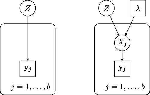
This approach to constructing an artificial joint target density is easily extended to accommodate random effects models, in which the original statistical model itself contains local variables associated with each data subset. These variables may be retained in the resulting instrumental model, alongside the local proxies $X_{1:b}$ for Z. A full description of the resulting model is presented in Rendell (2020).

The framework we describe is motivated by concepts in distributed optimization, a connection that is also explored in the contemporaneous work of Vono, Dobigeon, and Chainais (2019). The global consensus optimization problem (see, e.g., Boyd et al. 2011, sec. 7) is that of minimizing a sum of functions on a common domain, under the constraint that their arguments are all equal to some global common value. If for each $j\in \{1,\dots ,b\}$ one uses the Gaussian kernel density $K_j^{(\lambda )}(z,x)=\mathcal{N}(x;z,\lambda )$, then taking the negative logarithm of (2) gives (5) $$\begin{array}{c}-\hspace{0.17em}\text{log}\hspace{0.17em}{\tilde{\pi }}_{\lambda }(z,x_{1:b})=C-\hspace{0.17em}\text{log}\hspace{0.17em}\mu (z)\\ \hspace{1em}-\sum _{j=1}^b\hspace{0.17em}\text{log}\hspace{0.17em}{f}_j(x_j)+\frac{1}{2\lambda }\sum _{j=1}^b{\left(z-x_j\right)}^2,\end{array}$$(5) where C is a normalizing constant. Maximizing $\pi (z)$ is equivalent to minimizing this function under the constraint that $z=x_j$ for $j\in \{1,\dots ,b\}$, which may be achieved using the alternating direction method of multipliers (Bertsekas and Tsitsiklis 1989). Specifically, (5) corresponds to the use of $1/\lambda$ as the penalty parameter in this procedure.

There are some similarities between this framework and approximate Bayesian computation (ABC; see Marin et al. 2012, for a review of such methods). In both cases, one introduces a kernel that can be viewed as acting to smooth the likelihood. In the case of (2), the role of λ is to control the scale of smoothing that occurs in the parameter space; the tolerance parameter used in ABC, in contrast, controls the extent of a comparable form of smoothing in the observation (or summary statistic) space.

2.2 Distributed Metropolis-Within-Gibbs

The instrumental model described forms the basis of our proposed global consensus framework; “global consensus Monte Carlo” (GCMC) is correspondingly the application of Monte Carlo methods to form an approximation of ${\pi }_{\lambda }$. We focus here on the construction of a Metropolis-within-Gibbs Markov kernel that leaves ${\tilde{\pi }}_{\lambda }$ invariant. If λ is chosen to be sufficiently small, then the Z-marginal provides an approximation of π. Therefore given a chain with values denoted $(Z^i,X_{1:b}^i)$ for $i\in \{1,\dots ,N\}$, an empirical approximation of π is given by (6) $${\pi }_{\lambda }^N:=\frac{1}{N}\sum _{i=1}^N{\delta }_{Z^i},$$(6) where δ_z denotes the Dirac measure at z.

The Metropolis-within-Gibbs kernel we consider uses the full conditional densities (7) $${\tilde{\pi }}_{\lambda }(x_j|z)\propto K_j^{(\lambda )}(z,x_j)f_j(x_j)$$(7)

for $j\in \{1,\dots ,b\}$, and (8) $${\tilde{\pi }}_{\lambda }(z|x_{1:b})\propto \mu (z)\prod _{j=1}^b{K}_j^{(\lambda )}(z,x_j),$$(8) where (7) follows from the mutual conditional independence of $X_{1:b}$ given Z. Here, we observe that $K_j^{(\lambda )}(z,x_j)$ simultaneously provides a pseudo-prior for X_j and a pseudo-likelihood for Z.

We define $M_1^{(\lambda )}$ to be a ${\tilde{\pi }}_{\lambda }$-invariant Markov kernel that fixes z; we may write (9) $$M_1^{(\lambda )}((z,x_{1:b}); \mathrm{d}(z\prime ,x_{1:b}^{\prime }))={\delta }_z( \mathrm{d}z\prime )\prod _{j=1}^b{P}_{j,z}^{(\lambda )}(x_j, \mathrm{d}{x}_j^{\prime }),$$(9)

where for each j, $P_{j,z}^{(\lambda )}(x_j,·)$ is a Markov kernel leaving (7) invariant. We similarly define $M_2^{(\lambda )}$ to be a ${\tilde{\pi }}_{\lambda }$-invariant Markov kernel that fixes $x_{1:b}$, (10) $$M_2^{(\lambda )}((z,x_{1:b}); \mathrm{d}(z\prime ,x_{1:b}^{\prime }))=\left[\prod _{j=1}^b{\delta }_{x_j}( \mathrm{d}{x}_j^{\prime })\right]P_{x_{1:b}}^{(\lambda )}(z, \mathrm{d}z\prime ),$$(10) where $P_{x_{1:b}}^{(\lambda )}(z,·)$ is a Markov kernel leaving (8) invariant.

Using these Markov kernels, we construct an MCMC kernel that leaves ${\tilde{\pi }}_{\lambda }$ invariant; we present the resulting sampling procedure as Algorithm 1. In the special case in which one may sample exactly from the conditional distributions (7) and (8), this algorithm takes the form of a Gibbs sampler.

Algorithm 1

Global consensus Monte Carlo: MCMC algorithm

Fix $\lambda >0$. Set initial state $(Z^0,X_{1:b}^0)$; choose chain length N.

For $i=1,\dots ,N$:

• For $j\in \{1,\dots ,b\}$, sample $X_j^i\sim P_{j,Z^{i-1}}^{(\lambda )}(X_j^{i-1},·)$.

• Sample $Z^i\sim P_{X_{1:b}^i}^{(\lambda )}(Z^{i-1},·)$.

Return ${(Z^i,X_{1:b}^i)}_{i=1}^N$.

The interest from a distributed perspective is that the full conditional density (7) of each X_j , for given values x_j and z, depends only on the jth block of data (through the partial likelihood f_j ) and may be computed on the jth machine. Within Algorithm 1, the sampling of each $X_j^i$ from $P_{j,Z^{i-1}}^{(\lambda )}(X_j^{i-1},·)$ may therefore occur on the jth machine; these $X_{1:b}^i$ may then be communicated to a central machine that draws Zⁱ .

Our approach has particular benefits when sampling exactly from (7) is not possible, in which case Algorithm 1 takes a Metropolis-within-Gibbs form. One may choose the Markov kernels $P_{j,z}^{(\lambda )}$ to comprise multiple iterations of an MCMC kernel leaving (7) invariant; indeed multiple computations of each f_j (and therefore multiple accept/reject steps) may be conducted on each of the b nodes, without requiring communication between machines. This stands in contrast to more straightforward MCMC approaches directly targeting π, in which such communication is required for each evaluation of (1), and therefore for every accept/reject step. Similar to such a “direct” MCMC approach, each iteration of Algorithm 1 requires communication to and from each of the b machines on which the data are stored; but in cases where the communication latency is high, the resulting sampler will spend a greater proportion of time exploring the state space. This may in turn result in faster mixing (e.g., with respect to wall-clock time). We further discuss this comparison, and the role of communication latency, in Section S1.1 of the supplementary materials.

The setting in which Algorithm 1 describes a Gibbs sampler, with all variables drawn exactly from their full conditional distributions, is particularly amenable to analysis. We provide such a study in Section S2 of the supplementary materials. This analysis may also be informative about the more general Metropolis-within-Gibbs setting, when $P_{j,z}^{(\lambda )}$ comprises enough MCMC iterations to exhibit good mixing.

2.3 Choosing the Regularization Parameter

For $\phi :E\to \mathbb{R}$, we may estimate $\pi (\phi )$ using (6) as ${\pi }_{\lambda }^N(\phi )$. The regularization parameter λ here takes the role of a tuning parameter; we can view its effect on the mean squared error of such estimates using the bias–variance decomposition, (11) $$\mathbb{E}\mathrm{}\left[{\left({\pi }_{\lambda }^N(\phi )-\pi (\phi )\right)}^2\right]={[{\pi }_{\lambda }(\phi )-\pi (\phi )]}^2+\text{var}[{\pi }_{\lambda }^N(\phi )],$$(11) which holds exactly when $\mathbb{E}[{\pi }_{\lambda }^N(\phi )]={\pi }_{\lambda }(\phi )$. In many practical cases, this decomposition will provide a very accurate approximation for large N, as the squared bias of ${\pi }_{\lambda }^N(\phi )$ is typically asymptotically negligible in comparison to its variance.

The decomposition (11) separates the contributions to the error from the bias introduced by the instrumental model and the variance associated with the MCMC approximation. If λ is too large, the squared bias term in (11) can dominate while if λ is too small, the Markov chain may exhibit poor mixing due to strong conditional dependencies between $X_{1:b}$ and Z, and so the variance term in (11) can dominate.

It follows that λ should ideally be chosen to balance these two considerations. We provide a theoretical analysis of the role of λ in Section S2 of the supplementary materials, by considering a simple Gaussian setting. In particular, we show that for a fixed number of data, one should scale λ with the number of samples N as $\mathcal{O}(N^{-1/3})$ to minimize the mean squared error. We also consider the consistency of the approximate posterior ${\pi }_{\lambda }$ as the number of data n tends to infinity. Specifically, suppose these are split equally into b blocks; considering λ and b as functions of n, we find that ${\pi }_{\lambda }$ exhibits posterior consistency if $\lambda /b$ decreases to 0 as $n\to \infty$, and that credible intervals have asymptotically correct coverage if $\lambda /b$ decreases at a rate strictly faster than $n^{-1}$.

As an alternative to selecting a single value of λ, we propose in Section 3 a SMC sampler employing Markov kernels formed via Algorithm 1. In this manner, a decreasing sequence of λ values may be considered, which may result in lower-variance estimates for small λ values; we also describe a possible bias correction technique.

2.4 Related Approaches

As previously mentioned, a Gibbs sampler construction essentially corresponding to Algorithm 1 has independently been proposed by Vono, Dobigeon, and Chainais (2019). Their main objective is to improve algorithmic performance when computation of the full posterior density is intensive by constructing full conditional distributions that are more computationally tractable, for which they primarily consider a setting in which b = 1. In contrast, we focus on the exploitation of this framework in distributed settings (i.e., with b > 1), in the manner described in Section 2.2.

The objectives of our algorithm are similar, but not identical, to those of the previously introduced “embarrassingly parallel” approaches proposed by many authors. These reduce the costs of communication latency to a near-minimum by simulating a separate MCMC chain on each machine; typically, the chain on the jth machine is invariant with respect to a “subposterior” distribution with density proportional to $\mu {(z)}^{1/b}{f}_j(z)$. Communication is necessary only for the final aggregation step, in which an approximation of the full posterior is obtained using the samples from all b chains.

A well-studied approach within this framework is CMC (Scott et al. 2016), in which the post-processing step amounts to forming a “consensus chain” by weighted averaging of the separate chains. In the case that each subposterior density is Gaussian this approach can be used to produce samples asymptotically distributed according to π, by weighting each chain using the precision matrices of the subposterior distributions. Motivated by Bayesian asymptotics, the authors suggest using this approach more generally. In cases where the subposterior distributions exhibit near-Gaussianity this performs well, with the final “consensus chain” providing a good approximation of posterior expectations. However, there are no theoretical guarantees associated with this approach in settings in which the subposterior densities are poorly approximated by Gaussians. In such cases, CMC sometimes performs poorly in forming an approximation of the posterior π (as in examples of Wang et al. 2015; Srivastava et al. 2015; Dai, Pollock, and Roberts 2019), and so the resulting estimates of integrals $\pi (\phi )$ exhibit high bias.

Various authors (e.g., Minsker et al. 2014; Rabinovich, Angelino, and Jordan 2015; Srivastava et al. 2015; Wang et al. 2015) have therefore proposed alternative techniques for utilizing the values from each of these chains to approximate posterior expectations, each of which presents benefits and drawbacks. For example, Neiswanger, Wang, and Xing (2014) proposed a strategy based on kernel density estimation; based on this approach, Scott (2017) suggested a strategy based on finite mixture models, though notes that both methods may be impractical in high-dimensional settings.

An aggregation procedure proposed by Wang and Dunson (2013) bears some relation to our proposed framework, being based on the application of Weierstrass transforms to each subposterior density. The resulting smoothed densities are analogous to (3), which represents a smoothed form of the partial likelihood f_j . As well as proposing an aggregation method based on rejection sampling, the authors propose a technique for “refining” an initial posterior approximation, which may be expressed in terms of a Gibbs kernel on an extended state space. Comparing with our framework, this is analogous to applying Algorithm 1 for one iteration with N different initial values.

A potential issue common to these approaches is the treatment of the prior density μ. Each subposterior density is typically assigned an equal share of the prior information in the form of a fractionated prior density $\mu {(z)}^{1/b}$, but it is not clear when this approach is satisfactory. For example, suppose μ belongs to an exponential family; any property that is not invariant to multiplying the canonical parameters by a constant will not be preserved in the fractionated prior. As such if $\mu {(z)}^{1/b}$ is proportional to a valid probability density function of z, then the corresponding distribution may be qualitatively very different to the full prior. Although Scott et al. (2016) noted that fractionated priors perform poorly on some examples (for which tailored solutions are provided), no other general way of assigning prior information to each block naturally presents itself. In contrast our approach avoids this problem entirely, with μ providing prior information for Z at the “global” level.

Finally, we believe this work is complementary to other distributed algorithms lying outside of the “embarrassingly parallel” framework (including Xu et al. 2014; Jordan, Lee, and Yang 2019), and to approaches that aim to reduce the amount of computation associated with each likelihood calculation on a single node, for example, by using only a subsample or batch of the data (as in Korattikara, Chen, and Welling 2014; Bardenet, Doucet, and Holmes 2014; Huggins, Campbell, and Broderick 2016; Maclaurin and Adams 2014).

3 SMC Approach

As discussed in Section 2.3, as λ approaches 0 estimators ${\pi }_{\lambda }^N(\phi )$ formed using (6) exhibit lower bias but higher variance, due to poorer mixing of the resulting Markov chain. To obtain lower-variance estimators for λ values close to 0, we consider the use of SMC methodology to generate suitable estimates for a sequence of λ values.

SMC methodology employs sequential importance sampling and resampling; recent surveys include Doucet and Johansen (2011) and Doucet and Lee (2018). We consider here approximations of a sequence of distributions with densities ${\tilde{\pi }}_{{\lambda }_0},{\tilde{\pi }}_{{\lambda }_1},\dots$, where ${\lambda }_0,\dots ,{\lambda }_n$ is a decreasing sequence. The procedure we propose, specified in Algorithm 2, is an SMC sampler within the framework of Del Moral, Doucet, and Jasra (2006). This algorithmic form was first proposed by Gilks and Berzuini (2001) and Chopin (2002) in different settings, building upon ideas in Crooks (1998) and Neal (2001).

Algorithm 2

Global consensus Monte Carlo: SMC algorithm

Fix a decreasing sequence $({\lambda }_0,{\lambda }_1,\dots ,{\lambda }_n)$. Set number of particles N.

Initialize:

• For $i\in \{1,\dots ,N\}$, sample ${\zeta }_0^i=(Z_0^i,X_{0,1:b}^i)\sim {\tilde{\pi }}_{{\lambda }_0}$ and set $W_0^i\leftarrow 1$.

For $p=1,\dots ,n$:

1. For $i\in \{1,\dots ,N\}$, set ${\tilde{W}}_p^i\leftarrow W_{p-1}^i{w}_p({\zeta }_{p-1}^i)$, where $$w_p(z,x_{1:b}):=\frac{{\tilde{\pi }}_{{\lambda }_p}(z,x_{1:b})}{{\tilde{\pi }}_{{\lambda }_{p-1}}(z,x_{1:b})}=\prod _{j=1}^b\frac{K_j^{({\lambda }_p)}(z,x_j)}{K_j^{({\lambda }_{p-1})}(z,x_j)}.$$

2. Optionally, carry out a resampling step: for $i\in \{1,\dots ,N\}$,

   • Independently sample $A_{p-1}^i$ from the categorical distribution with probabilities proportional to $({\tilde{W}}_p^1,\dots ,{\tilde{W}}_p^N)$.

   • Set $W_p^i\leftarrow 1$.

Otherwise: for $i\in \{1,\dots ,N\}$ set $A_{p-1}^i\leftarrow i,W_p^i\leftarrow {\tilde{W}}_p^i$.

1. For $i\in \{1,\dots ,N\}$, sample ${\zeta }_p^i=(Z_p^i,X_{p,1:b}^i)\sim M_p({\zeta }_{p-1}^{A_{p-1}^i},·)$, where M_p is a ${\tilde{\pi }}_{{\lambda }_p}$-invariant MCMC kernel constructed in the manner of Algorithm 1.

2. Optionally, store the particle approximation of ${\tilde{\pi }}_{{\lambda }_p}$, $${\tilde{\pi }}_{{\lambda }_p}^N:=\frac{\sum _{i=1}^N{W}_p^i{\delta }_{{\zeta }_p^i}}{\sum _{i=1}^N{W}_p^i}.$$

The algorithm presented involves simulating particles using ${\tilde{\pi }}_{\lambda }$-invariant Markov kernels, and has a genealogical structure imposed by the ancestor indices $A_p^i$ for $p\in \{0,\dots ,n-1\}$ and $i\in \{1,\dots ,N\}$. The specific scheme for simulating the ancestor indices here is known as multinomial resampling; other schemes can be used (see Douc, Cappé, and Moulines 2005; Gerber, Chopin, and Whiteley 2019, for a summary of some schemes and their properties). We use this simple scheme here as it validates the use of the variance estimators used in Section 3.1. This optional resampling step is used to prevent the degeneracy of the particle set; a common approach is to carry out this step whenever the particles’ effective sample size (Liu and Chen 1995) falls below a predetermined threshold.

Under weak conditions ${\tilde{\pi }}_{{\lambda }_p}^N(\phi )$ converges almost surely to ${\tilde{\pi }}_{{\lambda }_p}(\phi )$ as $N\to \infty$. One can also define the particle approximations of ${\pi }_{{\lambda }_p}$ via (12) $${\pi }_{{\lambda }_p}^N:=\frac{\sum _{i=1}^N{W}_p^i{\delta }_{Z_p^i}}{\sum _{i=1}^N{W}_p^i},$$(12) where $Z_p^i$ is the first component of the particle ${\zeta }_p^i$.

Although the algorithm is specified for simplicity in terms of a fixed sequence ${\lambda }_0,\dots ,{\lambda }_n$, a primary motivation for the SMC approach is that the sequence used can be determined adaptively while running the algorithm. A number of such procedures have been proposed in the literature in the context of tempering, allowing each value λ_p to be selected based on the particle approximation of ${\tilde{\pi }}_{{\lambda }_{p-1}}$. For example, Jasra et al. (2011) proposed a procedure that controls the decay of the particles’ effective sample size. Within the examples in Section 4 we employ a procedure proposed by Zhou, Johansen, and Aston (2016), which generalizes this approach to settings in which resampling is not conducted in every iteration, aiming to control directly the dissimilarity between successive distributions. A possible approach to determining when to terminate the procedure, based on minimizing the mean squared error (11), is detailed in Section S3.2 of the supplementary materials.

With regard to initialization, if it is not possible to sample from ${\tilde{\pi }}_{{\lambda }_0}$ one could instead use samples obtained by importance sampling, or one could initialize an SMC sampler with some tractable distribution and use tempering or similar techniques to reach ${\tilde{\pi }}_{{\lambda }_0}$. At the expense of the introduction of an additional approximation, an alternative would be to run a ${\tilde{\pi }}_{{\lambda }_0}$-invariant Markov chain, and obtain an initial collection of particles by thinning the output (an approach that may be validated using results of Finke, Doucet, and Johansen 2020). Specifically, one could use Algorithm 1 to generate such samples for some large λ ₀, benefiting from its good mixing and low autocorrelation when λ is sufficiently large. The effect of Algorithm 2 may then be seen as refining or improving the resulting estimators, by bringing the parameter λ closer to zero.

Other points in favor of this approach are that many of the particle approximations (12) can be used to form a final estimate of $\pi (\phi )$ as explored in Section 3.1, and that SMC methods can be more robust to multimodality of π than simple Markov chain schemes. We finally note that in such an SMC sampler, a careful implementation of the MCMC kernels used may allow the inter-node communication to be interleaved with likelihood computations associated with the particles, thereby reducing the costs associated with communication latency.

3.1 Bias Correction Using Local Linear Regression

We present an approach to use many of the particle approximations produced by Algorithm 2. A natural idea is to regress the values of ${\pi }_{\lambda }^N(\phi )$ on λ, extrapolating to λ = 0 to obtain an estimate of $\pi (\phi )$. A similar idea has been used for bias correction in the context of ABC, albeit not in an SMC setting, regressing on the discrepancy between the observed data and simulated pseudo-observations (Beaumont, Zhang, and Balding 2002; Blum and François 2010).

Under very mild assumptions on the transition densities $K_j^{(\lambda )},{\pi }_{\lambda }(\phi )$ is smooth as a function of λ. Considering a first-order Taylor expansion of this function, a simple approach is to model the dependence of ${\pi }_{\lambda }(\phi )$ on λ as linear, for λ sufficiently close to 0. Having determined a subset of the values of λ used for which a linear approximation is appropriate (we propose a heuristic approach in Section S3.1 of the supplementary materials) one can use linear least squares to carry out the regression. To account for the SMC estimates ${\pi }_{{\lambda }_p}^N(\phi )$ having different variances, we propose the use of weighted least squares, with the “observations” ${\pi }_{{\lambda }_p}^N(\phi )$ assigned weights inversely proportional to their estimated variances; we describe methods for computing such variance estimates in Section 3.2. A bias-corrected estimate of $\pi (\phi )$ is then obtained by extrapolating the resulting fit to λ = 0, which corresponds to taking the estimated intercept term.

To make this explicit, first consider the case in which $\phi :E\to \mathbb{R}$, so that the estimates ${\pi }_{\lambda }^N(\phi )$ are univariate. For each value λ_p denote the corresponding SMC estimate by ${\eta }_p:={\pi }_{{\lambda }_p}^N(\phi )$, and let v_p denote some proxy for the variance of this estimate. Then for some set of indices $S:=\{p^{*},\dots ,n\}$ chosen such that the relationship between η_p and λ_p is approximately linear for $p\in S$, a bias-corrected estimate for $\pi (\phi )$ may be computed as (13) $${\pi }_S^{\text{BC}}(\phi ):={\tilde{\eta }}_S-{\tilde{\lambda }}_S\frac{\sum _{p\in S}({\lambda }_p-{\tilde{\lambda }}_S)({\eta }_p-{\tilde{\eta }}_S)/v_p}{\sum _{p\in S}{({\lambda }_p-{\tilde{\lambda }}_S)}^2/v_p},$$(13) where ${\tilde{\lambda }}_S$ and ${\tilde{\eta }}_S$ denote weighted means given by (14) $${\tilde{\lambda }}_S:=\frac{\sum _{p\in S}{\lambda }_p/v_p}{\sum _{p\in S}1/v_p},\hspace{1em}{\tilde{\eta }}_S:=\frac{\sum _{p\in S}{\eta }_p/v_p}{\sum _{p\in S}1/v_p}.$$(14)

The formal justification of this estimate assumes that the observations are uncorrelated, which does not hold here. We demonstrate in Section 4 and in Section S4.1 of the supplementary materials examples on which this simple approach is nevertheless effective, but in principle one could use generalized least squares combined with some approximation of the full covariance matrix of the SMC estimates.

In the more general case where $\phi :E\to {\mathbb{R}}^d$ for d > 1, we propose simply evaluating (13) for each component of this quantity separately, which corresponds to fitting an independent weighted least squares regression to each component. This facilitates the use of the variance estimators described in the following section, though in principle one could use multivariate weighted least squares or other approaches.

3.2 Variance Estimation for Weighted Least Squares

We propose the weighted form of least squares here since, as the values of λ used in the SMC procedure approach zero, the estimators generated may increase in variance: partly due to poorer mixing of the MCMC kernels as previously described, but also due to the gradual degeneracy of the particle set. To estimate the variances of estimates generated using SMC, several recent approaches have been proposed that allow this estimation to be carried out online by considering the genealogy of the particles. Using any such procedure, one may estimate the variance of ${\pi }_{\lambda }^N(\phi )$ for each λ value considered by Algorithm 2, with these values used for each v_p in (13).

Within our examples, we use the estimator proposed by Lee and Whiteley (2018), which for fixed N coincides with an earlier proposal of Chan and Lai (2013) (up to a multiplicative constant). Specifically, after each step of the SMC sampler we compute an estimate of the asymptotic variance of each estimate ${\pi }_{{\lambda }_p}^N(\phi )$; that is, the limit of $N\text{var}[{\pi }_{{\lambda }_p}^N(\phi )]$ as $N\to \infty$. While this is not equivalent to computing the true variance of each estimate, for fixed large N the relative sizes of these asymptotic variance estimates should provide a useful indicator of the relative variances of each estimate ${\pi }_{\lambda }^N(\phi )$. In Section S4.1 of the supplementary materials, we show empirically that inversely weighting the SMC estimates according to these estimated variances can result in more stable bias-corrected estimates as the particle set degenerates. We also explain in Section S3.2 how these estimated variances can be used within a rule to determine when to terminate the algorithm.

The asymptotic variance estimator described is consistent in N. However, if in practice resampling at the pth time step causes the particle set to degenerate to having a single common ancestor, then the estimator evaluates to zero, and so it is impossible to use this value as the inverse weight v_p in (13). Such an outcome may be interpreted as a warning that too few particles have been used for the resulting SMC estimates to be reliable, and that a greater number should be used when rerunning the procedure.

4 Examples

4.1 Log-Normal Toy Example

To compare the posterior approximations formed by our global consensus framework with those formed by some embarrassingly parallel approaches discussed in Section 2.4, we conduct a simulation study based on a simple model. Let $\mathcal{L}\mathcal{N}(x;\mu ,{\sigma }^2)$ denote the density of a log-normal distribution with parameters $(\mu ,{\sigma }^2)$; that is, $$\mathcal{L}\mathcal{N}(x;\mu ,{\sigma }^2)=\frac{1}{x\sqrt{2\pi {\sigma }^2}}\text{exp}\hspace{0.17em}\left(-\frac{{(\hspace{0.17em}\text{log}\hspace{0.17em}(x)-\mu )}^2}{2{\sigma }^2}\right).$$

One may consider a model with prior density $\mu (z)=\mathcal{L}\mathcal{N}(z;{\mu }_0,{\sigma }_0^2)$ and likelihood contributions $f_j(z)=\mathcal{L}\mathcal{N}(\hspace{0.17em}\text{log}\hspace{0.17em}({\mu }_j);\hspace{0.17em}\text{log}\hspace{0.17em}(z),{\sigma }_j^2)$ for $j\in \{1,\dots ,b\}$. This may be seen as a reparameterization of the Gaussian model in Section S2 of the supplementary materials, in which each likelihood contribution is that of a data subset with a Gaussian likelihood. This convenient setting allows for the target distribution π to be expressed analytically. For the implementation of the global consensus algorithm, we choose Markov transition kernels given by $K_j^{(\lambda )}(z,x)=\mathcal{L}\mathcal{N}(x;\hspace{0.17em}\text{log}\hspace{0.17em}(z),\lambda )$ for each $j\in \{1,\dots ,b\}$, which satisfy Assumption 1; this allows for exact sampling from all the full conditional distributions.

As a toy example to illustrate the effects of non-Gaussian partial likelihoods we consider a case in which $f_j(z)=\mathcal{L}\mathcal{N}(\hspace{0.17em}\text{log}\hspace{0.17em}({\mu }_j);\hspace{0.17em}\text{log}\hspace{0.17em}(z),1)$ for each j, and $\mu (z)=\mathcal{L}\mathcal{N}(z;0,25)$. Here we took b = 32, and selected the location parameters μ_j as iid samples from a standard normal distribution. We ran GCMC using the Gibbs sampler form of Algorithm 1, for values of λ between ${10}^{-5}$ and 10. For comparison, we also drew samples from each subposterior distribution as defined in Section 2.4, combining the samples using various approaches. These are the CMC averaging of Scott et al. (2016); the nonparametric density product estimation (NDPE) approach of Neiswanger, Wang, and Xing (2014); and the Weierstrass rejection sampling (WRS) combination technique of Wang and Dunson (2013), using their R implementation (https://github.com/wwrechard/weierstrass). In each case, we ran the algorithm 25 times, drawing $N={10}^5$ samples.

To demonstrate the role of λ in the bias–variance decomposition (11), Table 1 presents the means and standard deviations of estimates of $\pi (\phi )$, for various test functions $\phi$. In estimating the first moment of π, GCMC generates a low-bias estimator when λ is chosen to be sufficiently small; however, as expected, the variance of such estimators increases when very small values of λ are chosen. While the other methods produce estimators of reasonably low variance, these exhibit somewhat higher bias. For CMC, the bias is especially pronounced when estimating higher moments of the posterior distribution, as exemplified by the estimates of the fifth moment. Note however that high biases are also introduced when using GCMC with large values of λ (as seen here with λ = 10), for which ${\pi }_{\lambda }$ is a poor approximation of π.

Table 1 True values and estimates of $\pi (\phi )$, for various test functions $\phi$, for the log-normal toy model.

		$\phi (z)=z$	$\phi (z)=z^5$	$\phi (z)=\hspace{0.17em}\text{log}\hspace{0.17em}(z)$
Algorithm		($\pi (\phi )=1.141$)	($\pi (\phi )=2.644$)	($\pi (\phi )=0.1164$)
GCMC	$\lambda ={10}^1$	1.329 ± 0.003	121.154 ± 10.487	0.1151 ± 0.0019
	$\lambda ={10}^0$	1.159 ± 0.002	3.901 ± 0.037	$0.1165\pm 0.0014$
	$\lambda ={10}^{-1}$	$1.144\pm 0.003$	$2.763\pm 0.044$	0.1173 ± 0.0030
	$\lambda ={10}^{-2}$	1.140 ± 0.011	2.648 ± 0.143	0.1150 ± 0.0090
	$\lambda ={10}^{-3}$	1.142 ± 0.022	2.661 ± 0.295	0.1191 ± 0.0199
	$\lambda ={10}^{-4}$	1.120 ± 0.077	3.505 ± 1.136	0.1630 ± 0.0651
	$\lambda ={10}^{-5}$	1.400 ± 0.110	6.195 ± 2.217	0.3283 ± 0.0810
CMC		1.073 ± 0.010	16.092 ± 5.675	0.0135 ± 0.0095
NDPE		1.148 ± 0.029	2.800 ± 0.385	0.1231 ± 0.0246
WRS		1.111 ± 0.007	2.444 ± 0.086	0.0862 ± 0.0063

NOTE: Estimates obtained using global consensus Monte Carlo with various values of λ, and three embarrassingly parallel methods (see main text for abbreviations). For each method the mean estimate ± Monte Carlo standard error is presented, as computed over 25 replicates; the estimator corresponding to the lowest mean squared error is printed in bold.

Also of note are estimates of $\int \hspace{0.17em}\text{log}\hspace{0.17em}(z)\pi (z) \mathrm{d}z$, corresponding to the mean of the Gaussian model of which this a reparameterization. While GCMC performs well across a range of λ values, the other methods perform less favorably; CMC produces an estimate that is incorrect by an order of magnitude. While this could be solved by a simple reparameterization of the problem in this case, in more general settings no such straightforward solution may exist.

In Section S4.2 of the supplementary materials, we present second example based on a log-normal model, demonstrating the robustness of these methods to permutation and repartitioning of the data.

4.2 Logistic Regression

Binary logistic regression models are commonly used in settings related to marketing. In web design for example, A/B testing may be used to determine which content choices lead to maximized user interaction, such as the user clicking on a product for sale.

We assume that we have a dataset of size n formed of responses ${\eta }_l\in \{-1,1\}$, and vectors ${\xi }_l\in {\{0,1\}}^d$ of binary covariates, where $l\in \{1,\dots ,n\}$. The likelihood contribution of each block of data then takes the form $f_j(z)=\prod _{l}S({\eta }_l{z}^T{\xi }_l),z\in {\mathbb{R}}^d$, where the product is taken over those indices l included in the jth block of data, and S denotes the logistic function, $S(x)={(1+\hspace{0.17em}\text{exp}\hspace{0.17em}(x))}^{-1}$.

For the prior μ, we use a product of independent zero-mean Gaussians, with standard deviation 20 for the parameter corresponding to the intercept term, and 5 for all other parameters. For the Markov transition densities in GCMC, we use multivariate Gaussian densities: $K_j^{(\lambda )}(z,x)=\mathcal{N}(x;z,\lambda I)$ for each $j\in \{1,\dots b\}$.

We investigated several such simulated datasets and the efficacy of various approaches in approximating the true posterior π. To illustrate the bias–variance trade-off described in Section 2.3, in the presentation of these results we focus on the estimation of the posterior first moment; denoting the identity function on ${\mathbb{R}}^d$ by $\text{Id}$, we may write this as $\pi (\text{Id})$. While our global consensus approach was consistently successful in forming estimators with low mean squared error in each component, in low-dimensional settings the application of CMC often resulted in marginal improvements. However, in many higher-dimensional settings, the estimators resulting from CMC exhibited relatively large biases.

We present here an example in which the d predictors correspond to p binary input variables, their pairwise products, and an intercept term, so that $d=1+p+(\begin{array}{c}p\\ 2\end{array})$. In settings where the interaction effects corresponding to these pairwise products are of interest, the dimensionality d of the space can be very large compared to p. We used a simulated dataset with p = 20 input variables, resulting in a parameter space of dimension d = 211. The data comprise $n=80,000$ observations, split into b = 8 equally sized blocks. Each observation of the 20 binary variables was generated from a Bernoulli distribution with parameter 0.1, and for each vector of covariates, the response was generated from the correct model, for a fixed underlying parameter vector $z^{*}$.

4.2.1 Metropolis-Within-Gibbs

We applied GCMC for values of λ between ${10}^{-2}$ and 1. We used a Metropolis-within-Gibbs formulation of Algorithm 1, sampling directly from the Gaussian conditional distribution of Z given $X_{1:b}$. To sample approximately from the conditional distributions of each X_j given Z we used Markov kernels $P_{j,z}^{(\lambda )}$ comprising k = 20 iterations of a random walk Metropolis kernel.

As mentioned in Section 2.2, in settings of high communication latency our approach allows a greater proportion of wall-clock time to be spent on likelihood contributions, compared to an MCMC chain directly targeting the full posterior π. To compare across settings, we therefore consider an abstracted distributed setting as discussed in Section S1.1 of the supplementary materials, here assuming that the latency is 10 times the time taken to compute each partial likelihood f_j (in the notation of Section S1.1, $C=10\mathcal{l}$).

We also compare with the same embarrassingly parallel approaches as in Section 4.1 (CMC, NDPE, WRS), which are comparatively unaffected by communication latency. For these methods, we again used random walk Metropolis to draw samples from each subposterior distribution. To ease computation, we thinned these chains before applying the combination step; in practice, the estimators obtained using these thinned chains behaved very similarly to those obtained using all subposterior samples.

To provide a “ground truth” against which to compare the results we ran a random walk Metropolis chain of length $500,000$ targeting π. For all our random walk Metropolis samplers we used Gaussian proposal kernels. To determine the covariance matrices of these, we formed a Laplace approximation of the target density following the approach of Chopin and Ridgway (2017), scaling the resulting covariance matrix optimally according to results of Roberts and Rosenthal (2001).

For each algorithmic setting, we ran the corresponding sampler 25 times. To compare the resulting estimators of the posterior mean we computed the mean squared error of each of the d components of the posterior mean, summing these to obtain a “mean sum of squared errors.”

Table 2 compares the values obtained by each algorithm after an approximate wall-clock time equal to $200,000$ times the time taken to compute a single partial likelihood f_j . Accounting for latency in the abstracted distributed setting described above, the GCMC approach is able to generate 5000 approximate posterior samples during this time, spending 50% of time on likelihood computations. In contrast, a direct MCMC approach generates 9523 samples, but would only spend 4.8% of the time on likelihood computations, with the remainder lost due to latency.

Table 2 Mean sum of squared errors over all d components of estimates of the posterior mean for the logistic regression model, formed using various algorithmic approaches as described in the main text, during an approximate wall-clock time equal to $200,000$ times that required to compute a single partial likelihood f_j .

Algorithm		Mean sum of squared errors
GCMC	$\lambda ={10}^0$	0.1835
	$\lambda ={10}^{-0.5}$	0.1379
	$\lambda ={10}^{-1}$	0.0770
	$\lambda ={10}^{-1.5}$	$0.0478$
	$\lambda ={10}^{-2}$	0.0662
CMC		0.3710
NDPE		0.8476
WRS		0.6402
Direct MCMC		0.0884

NOTE: All values computed over 25 replicates, with the lowest value printed in bold.

The result is that the estimators generated by GCMC for appropriately chosen λ exhibit lower mean sums of squared errors: we conduct many more accept/reject steps in each round of inter-node communication than if we were to directly target π, and so it becomes possible to achieve faster mixing of the Z-chain (and a better estimator) compared to such a direct approach. This may be seen when comparing the effective sample size (ESS) of each chain, where we estimate this via the “batch means” approach of Vats, Flegal, and Jones (2019): we find that the average ESS of the direct MCMC chains is only 1111, while depending on the choice of λ, the shorter GCMC chains have average ESS values between 1327 and 4577.

Despite being unaffected by latency and therefore allowing many more samples to be drawn, the embarrassingly parallel approaches (CMC, NDPE, WRS) perform poorly compared to GCMC. This is particularly true of the NDPE method of Neiswanger, Wang, and Xing (2014): while asymptotically exact even in non-Gaussian settings, the resulting estimator is based on kernel density estimators and is not effective in this high-dimensional setting.

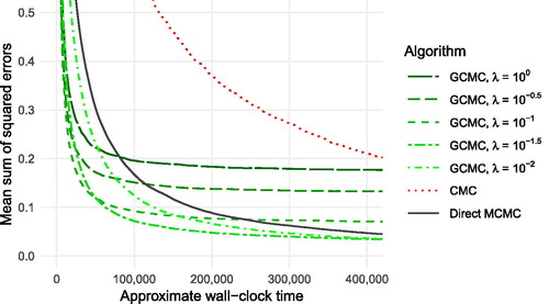
Figure 2 shows the mean sums of squared errors as a function of the approximate wall-clock time (for simplicity we include only the best-performing of the three embarrassingly parallel methods, omitting the results for NDPE and WRS). We see that for large enough λ, the GCMC estimators ${\pi }_{\lambda }^N(\text{Id})$ exhibit rather lower values than the corresponding CMC and “direct” MCMC estimators. As the number of samples used grows, the squared bias of these estimators begins to dominate, and so smaller λ values result in lower mean squared errors. As λ becomes smaller the autocorrelation of the resulting Z-chain increases; indeed we found that for λ too small, the GCMC estimator ${\pi }_{\lambda }^N(\text{Id})$ will always have a greater mean squared error than the “direct” MCMC estimator, no matter how much time is used. Of course, since an MCMC estimator formed by directly targeting π is consistent in N, given sufficient time such an estimator will always outperform estimators formed using GCMC, which are biased for any λ. However, in many practical big data settings it may be infeasible to draw large numbers of samples using the available time budget.

Fig. 2 Mean sum of squared errors over all d components of estimates of the posterior mean for the logistic regression model, formed using various algorithmic approaches as described in the main text. Values plotted against the approximate wall-clock time, relative to the time taken to compute a single partial likelihood term. All values computed over 25 replicates.

4.2.2 Sequential Monte Carlo

We also applied the SMC procedure to this logistic regression model. While we found that the SMC approach was most effective in lower-dimensional settings (see Section S4.1 of the supplementary materials for a simple example) in which it is less computationally expensive, the SMC procedure can be more widely useful as a means of “refining” the estimator formed using a single λ value, as discussed in Section 3.

We used N = 1250 particles, initializing the particle set by thinning the chain generated by the Metropolis-within-Gibbs procedure with $\lambda ={10}^{-1}$. To generate a sequence of subsequent λ values we used the adaptive procedure of Zhou, Johansen, and Aston (2016), using tuning parameter ${\text{CESS}}^{\star }=0.98$. For the Markov kernels M_p , we used Metropolis-within-Gibbs kernels as previously, with each update of X_j given Z comprising k = 50 iterations of a random walk Metropolis kernel.

The estimator ${\pi }_{{\lambda }_0}^N(\text{Id})$ formed using the initial particle set was found to have a mean sum of squared errors of 0.0692. After a fixed number of iterations (n = 100) the resulting SMC estimate exhibited a mean sum of squared errors of 0.0418; this represents a decrease of 40%, and has the benefit of avoiding the need to carefully specify a single value for λ.

Used alone, the bias correction procedure of Section 3.1 was found to perform best in lower-dimensional settings (as in Section S4.1 of the supplementary materials); here, it resulted in a mean sum of squared errors of 0.0682 after 100 iterations. However, improved results were obtained using the stopping rule we propose in Section S3.2 of the supplementary materials (with stopping parameter κ = 15), which is based on our proposed bias correction procedure. The estimator selected by this stopping rule, which automatically determines when to terminate the algorithm, obtained a mean sum of squared errors of 0.0367, a decrease of 47% from the estimator generated using the initial particle set.

5 Conclusion

We have presented a new framework for sampling in distributed settings, demonstrating its application on some illustrative examples in comparison to embarrassingly parallel approaches. Given that our proposed approach makes no additional assumptions on the form of the likelihood beyond its factorized form as in (1), we expect that our algorithm will be most effective in those big data settings for which approximate Gaussianity of the likelihood contributions may not hold. These may include high-dimensional settings, for which some subsets of the data may be relatively uninformative about the parameter. In such cases, the likelihood contributions may be highly non-Gaussian, so that the CMC approach of averaging across chains results in estimates of high bias; simultaneously, the high dimensionality may preclude the use of alternative combination techniques (e.g., the use of kernel density estimates).

This framework may be of use in serial settings. As previously noted, the contemporaneous work of Vono, Dobigeon, and Chainais (2019) presents an example in which the use of an analogous framework (with b = 1) results in more efficient simulation than approaches that directly target the true posterior. Our proposed SMC sampler implementation and the associated bias correction technique may equally be applied to such settings, reducing the need to specify a single value of the regularization parameter λ.

There is potential for further improvements to be made to the procedures we present here. In the SMC case for example, while our proposed use of weighted least squares as a bias correction technique is simple, nonlinear procedures (such those proposed in an ABC context by Blum and François 2010) may provide a more robust alternative, with some theoretical guarantees. We also stress that the MCMC and SMC procedures presented here constitute only two possible approaches to inference within the instrumental hierarchical model that we propose, and there is considerable scope for alternative sampling algorithms to be employed within this global consensus framework.

Supplementary Materials

Supplement to “Global consensus Monte Carlo”: “GCMCsupplement.pdf” includes supplementary materials covering implementation considerations, theoretical analysis for a simple model, and heuristic procedures for the proposed SMC sampler (with numerical demonstrations).

R code for examples: “GCMCexamples.zip” contains R scripts used to generate the numerical results and figures presented here and in the supplement.

Additional information

Funding

The authors gratefully acknowledge the support of The Alan Turing Institute under the EPSRC grant EP/N510129/1, the Lloyd’s Register Foundation–Alan Turing Institute Programme on Data-Centric Engineering, and the EPSRC under grants EP/M508184/1, EP/R034710/1 and EP/T004134/1.

References

- Bardenet, R. , Doucet, A. , and Holmes, C. (2014), “Towards Scaling Up Markov Chain Monte Carlo: An Adaptive Subsampling Approach,” in Proceedings of the 31st International Conference on Machine Learning (ICML-14 ), pp. 405–413.
- Beaumont, M. A. , Zhang, W. , and Balding, D. J. (2002), “Approximate Bayesian Computation in Population Genetics,” Genetics , 162, 2025–2035.
- Bertsekas, D. P. , and Tsitsiklis, J. N. (1989), Parallel and Distributed Computation: Numerical Methods , Englewood Cliffs, NJ: Prentice- Hall.
- Blum, M. G. , and François, O. (2010), “Non-Linear Regression Models for Approximate Bayesian Computation,” Statistics and Computing , 20, 63–73. DOI: 10.1007/s11222-009-9116-0.
- Boyd, S. , Parikh, N. , Chu, E. , Peleato, B. , and Eckstein, J. (2011), “Distributed Optimization and Statistical Learning via the Alternating Direction Method of Multipliers,” Foundations and Trends® in Machine Learning , 3, 1–122. DOI: 10.1561/2200000016.
- Chan, H. P. , and Lai, T. L. (2013), “A General Theory of Particle Filters in Hidden Markov Models and Some Applications,” The Annals of Statistics , 41, 2877–2904. DOI: 10.1214/13-AOS1172.
- Chopin, N. (2002), “A Sequential Particle Filter Method for Static Models,” Biometrika , 89, 539–552. DOI: 10.1093/biomet/89.3.539.
- Chopin, N. , and Ridgway, J. (2017), “Leave Pima Indians Alone: Binary Regression as a Benchmark for Bayesian Computation,” Statistical Science , 32, 64–87. DOI: 10.1214/16-STS581.
- Crooks, G. E. (1998), “Nonequilibrium Measurements of Free Energy Differences for Microscopically Reversible Markovian Systems,” Journal of Statistical Physics , 90, 1481–1487.
- Dai, H. , Pollock, M. , and Roberts, G. (2019), “Monte Carlo Fusion,” Journal of Applied Probability , 56, 174–191. DOI: 10.1017/jpr.2019.12.
- Dean, J. , and Ghemawat, S. (2008), “MapReduce: Simplified Data Processing on Large Clusters,” Communications of the ACM , 51, 107–113. DOI: 10.1145/1327452.1327492.
- Del Moral, P. , Doucet, A. , and Jasra, A. (2006), “Sequential Monte Carlo Samplers,” Journal of the Royal Statistical Society, Series B, 68, 411–436. DOI: 10.1111/j.1467-9868.2006.00553.x.
- Douc, R. , Cappé, O. , and Moulines, E. (2005), “Comparison of Resampling Schemes for Particle Filtering,” in Proceedings of the 4th International Symposium on Image and Signal Processing and Analysis , IEEE, pp. 64–69. DOI: 10.1109/ISPA.2005.195385.
- Doucet, A. , and Johansen, A. M. (2011), “A Tutorial on Particle Filtering and Smoothing: Fifteen Years Later,” in Handbook of Nonlinear Filtering , eds. D. Crisan and B. Rozovskii , Oxford: Oxford University Press, pp. 656–704.
- Doucet, A. , and Lee, A. (2018), “Sequential Monte Carlo methods,” in Handbook of Graphical Models , eds. M. Maathuis , M. Drton , S. L. Lauritzen , and M. Wainwright , Boca Raton, FL: CRC Press, pp. 165–189.
- Finke, A. , Doucet, A. , and Johansen, A. M. (2020), “Limit Theorems for Sequential MCMC Methods,” Advances in Applied Probability , 52, 377–403. DOI: 10.1017/apr.2020.9.
- Gerber, M. , Chopin, N. , and Whiteley, N. (2019), “Negative Association, Ordering and Convergence of Resampling Methods,” The Annals of Statistics , 47, 2236–2260. DOI: 10.1214/18-AOS1746.
- Gilks, W. R. , and Berzuini, C. (2001), “Following a Moving Target—Monte Carlo Inference for Dynamic Bayesian Models,” Journal of the Royal Statistical Society, Series B, 63, 127–146. DOI: 10.1111/1467-9868.00280.
- Huggins, J. , Campbell, T. , and Broderick, T. (2016), “Coresets for Scalable Bayesian Logistic Regression,” in Advances in Neural Information Processing Systems , pp. 4080–4088.
- Jasra, A. , Stephens, D. A. , Doucet, A. , and Tsagaris, T. (2011), “Inference for Lévy-Driven Stochastic Volatility Models via Adaptive Sequential Monte Carlo,” Scandinavian Journal of Statistics , 38, 1–22. DOI: 10.1111/j.1467-9469.2010.00723.x.
- Jordan, M. I. , Lee, J. D. , and Yang, Y. (2019), “Communication-Efficient Distributed Statistical Inference,” Journal of the American Statistical Association , 114, 668–681. DOI: 10.1080/01621459.2018.1429274.
- Korattikara, A. , Chen, Y. , and Welling, M. (2014), “Austerity in MCMC Land: Cutting the Metropolis-Hastings Budget, ” in Proceedings of the 31st International Conference on Machine Learning (ICML-14) .
- Lee, A. , and Whiteley, N. (2018), “Variance Estimation in the Particle Filter,” Biometrika , 105, 609–625. DOI: 10.1093/biomet/asy028.
- Liu, J. S. , and Chen, R. (1995), “Blind Deconvolution via Sequential Imputations,” Journal of the American Statistical Association , 90, 567–576. DOI: 10.1080/01621459.1995.10476549.
- Maclaurin, D. , and Adams, R. P. (2014), “ Firefly Monte Carlo: Exact MCMC With Subsets of Data,” in Proceedings of the 30th International Conference on Uncertainty in Artificial Intelligence (UAI-14 ), pp. 543–552.
- Marin, J. M. , Pudlo, P. , Robert, C. P. , and Ryder, R. J. (2012), “Approximate Bayesian Computational Methods,” Statistics and Computing , 22, 1167–1180. DOI: 10.1007/s11222-011-9288-2.
- Minsker, S. , Srivastava, S. , Lin, L. , and Dunson, D. (2014), “ Scalable and Robust Bayesian Inference via the Median Posterior,” in Proceedings of the 31st International Conference on Machine Learning (ICML-14 ), pp. 1656–1664.
- Neal, R. M. (2001), “Annealed Importance Sampling,” Statistics and Computing , 11, 125–139. DOI: 10.1023/A:1008923215028.
- Neiswanger, W. , Wang, C. , and Xing, E. (2014), “Asymptotically Exact, Embarrassingly Parallel MCMC,” in Proceedings of the 30th International Conference on Uncertainty in Artificial Intelligence (UAI-14 ), pp. 623–632.
- Rabinovich, M. , Angelino, E. , and Jordan, M. I. (2015), “Variational Consensus Monte Carlo,” in Advances in Neural Information Processing Systems , pp. 1207–1215.
- Rendell, L. J. (2020), “Sequential Monte Carlo Variance Estimators and Global Consensus,” Ph.D. thesis, University of Warwick.
- Rendell, L. J. , Johansen, A. M. , Lee, A. , and Whiteley, N. (2018), “Global Consensus Monte Carlo,” arXiv no. 1807.09288.
- Roberts, G. O. , and Rosenthal, J. S. (2001), “Optimal Scaling for Various Metropolis–Hastings Algorithms,” Statistical Science , 16, 351–367. DOI: 10.1214/ss/1015346320.
- Scheffé, H. (1947), “A Useful Convergence Theorem for Probability Distributions,” The Annals of Mathematical Statistics , 18, 434–438.
- Scott, S. L. (2017), “Comparing Consensus Monte Carlo Strategies for Distributed Bayesian Computation,” Brazilian Journal of Probability and Statistics , 31, 668–685. DOI: 10.1214/17-BJPS365.
- Scott, S. L. , Blocker, A. W. , Bonassi, F. V. , Chipman, H. A. , George, E. I. , and McCulloch, R. E. (2016), “Bayes and Big Data: The Consensus Monte Carlo Algorithm,” International Journal of Management Science and Engineering Management , 11, 78–88. DOI: 10.1080/17509653.2016.1142191.
- Srivastava, S. , Cevher, V. , Dinh, Q. , and Dunson, D. (2015), “WASP: Scalable Bayes via Barycenters of Subset Posteriors,” in Artificial Intelligence and Statistics , pp. 912–920.
- Vats, D. , Flegal, J. M. , and Jones, G. L. (2019), “Multivariate Output Analysis for Markov Chain Monte Carlo,” Biometrika , 106, 321–337. DOI: 10.1093/biomet/asz002.
- Vono, M. , Dobigeon, N. , and Chainais, P. (2018), “Sparse Bayesian Binary Logistic Regression Using the Split-and-Augmented Gibbs Sampler,” in Proceedings of the IEEE International Workshop on Machine Learning for Signal Processing .
- Vono, M. , Dobigeon, N. , and Chainais, P. (2019), “Split-and-Augmented Gibbs Sampler—Application to Large-Scale Inference Problems,” IEEE Transactions on Signal Processing , 67, 1648–1661.
- Vono, M. , Paulin, D. , and Doucet, A. (2019), “Efficient MCMC Sampling With Dimension-Free Convergence Rate Using ADMM-Type Splitting,” arXiv no. 1905.11937.
- Wang, X. , and Dunson, D. B. (2013), “Parallelizing MCMC via Weierstrass Sampler,” arXiv no. 1312.4605.
- Wang, X. , Guo, F. , Heller, K. A. , and Dunson, D. B. (2015), “Parallelizing MCMC With Random Partition Trees,” in Advances in Neural Information Processing Systems , pp. 451–459.
- Xu, M. , Lakshminarayanan, B. , Teh, Y. W. , Zhu, J. , and Zhang, B. (2014), “Distributed Bayesian Posterior Sampling via Moment Sharing,” in Advances in Neural Information Processing Systems , pp. 3356–3364.
- Zhou, Y. , Johansen, A. M. , and Aston, J. A. (2016), “Towards Automatic Model Comparison: An Adaptive Sequential Monte Carlo Approach,” Journal of Computational and Graphical Statistics , 25, 701–726. DOI: 10.1080/10618600.2015.1060885.