Subset Multivariate Collective and Point Anomaly Detection

Abstract

In the recent years, there has been a growing interest in identifying anomalous structure within multivariate data sequences. We consider the problem of detecting collective anomalies, corresponding to intervals where one, or more, of the data sequences behaves anomalously. We first develop a test for a single collective anomaly that has power to simultaneously detect anomalies that are either rare, that is affecting few data sequences, or common. We then show how to detect multiple anomalies in a way that is computationally efficient but avoids the approximations inherent in binary segmentation-like approaches. This approach is shown to consistently estimate the number and location of the collective anomalies—a property that has not previously been shown for competing methods. Our approach can be made robust to point anomalies and can allow for the anomalies to be imperfectly aligned. We show the practical usefulness of allowing for imperfect alignments through a resulting increase in power to detect regions of copy number variation. Supplemental files for this article are available online.

Keywords:

• Copy number variations
• Dynamic programming
• Epidemic changepoints
• Outliers
• Robust statistics

1 Introduction

The field of anomaly detection has attracted considerable attention in the recent years, in part due to an increasing need to automatically process large volumes of data gathered without human intervention. Interest is either in removing anomalies, so that robust inferences can be made by analyzing nonanomalous data (Rousseeuw and Bossche 2018), or detecting anomalies because they are indicative of features of interest. Examples of the latter include anomalous sensor measurements indicating failure of equipment (Cui, Bangalore, and Tjernberg 2018), or unusual patterns in computer network data indicating a cyber attack (Metelli and Heard 2019). Comprehensive reviews of the area can be found in Chandola, Banerjee, and Kumar (2009) and Pimentel et al. (2014). One of the main challenges in anomaly detection is that anomalies can come in different guises. Chandola, Banerjee, and Kumar (2009) categorized anomalies into one of three categories: global, contextual, or collective. The first two of these categories are point anomalies, that is, single observations which are anomalous with respect to the global, or local, data context, respectively. Conversely, a collective anomaly is defined as a sequence of observations which together form an anomalous pattern.

In this article, we focus on the following setting: we observe a multivariate time series ${\mathbf{x}}_1,\dots ,{\mathbf{x}}_n\in {\mathbb{R}}^p$ corresponding to observations at n discrete time-points, each across p different components. Each component of the series has a typical behavior, interspersed by windows of time where it behaves anomalously. In line with the definition in Chandola, Banerjee, and Kumar (2009), we call the behavior within such a time window a collective anomaly. Often the underlying cause of such a collective anomaly will affect more than one, but not necessarily all, of the components. Our aim is to accurately estimate the location of these collective anomalies within the multivariate series, potentially in the presence of point anomalies.

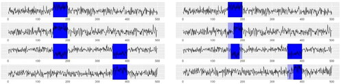
Whilst it may be mathematically convenient to assume that anomalous structure occurs contemporaneously across all affected sequences, in practice one might expect some time delays as illustrated in Figure 1. We will consider two different scenarios for the alignment of related collective anomalies across different components. First, that concurrent collective anomalies perfectly align. That is, we can segment our time series into windows of typical and anomalous behavior, with the latter affecting a subset of components. The second, and for many applications more realistic, setting assumes that concurrent collective anomalies start and end at similar but not necessarily identical time points.

Fig. 1 An example of time series with K = 2 collective anomalies, highlighted in blue, where they are perfectly aligned (left) and are mis-aligned (right). Using notation from Section 2 these collective anomalies occur from times $s_1=150$ to $e_1=200$ and $s_2=350$ to $e_2=400$; the affected components are ${\mathbf{J}}_1=\{1,2,3\}$ and ${\mathbf{J}}_2=\{3,4\}$. For the mis-aligned anomalies, the time series have anomalous behavior in dark-blue regions, and behave normally in light-blue regions.

There has been much less work on detecting collective anomalies than point anomalies. It is possible to use point anomaly methods to detect a collective anomaly, by applying them to data from suitably chosen periods of time. For example, Talagala, Hyndman, and Smith-Miles (2021) used this approach to detect anomalous daily behavior of pedestrians in Melbourne, while the online method of Talagala et al. (2020) produced a bivariate summary of data within a moving window and detects a collective anomaly based on a measure of how unusual this summary is. One problem with these approaches is the need to specify an appropriate period of time or window length.

Other approaches aimed at detecting collective anomalies include state space models and (epidemic) changepoint methods. State space models assume that a hidden state, which evolves following a Markov chain, determines whether the time series’ behavior is typical or anomalous. Examples of state space models for anomaly detection can be found in Smyth (1994) and Bardwell and Fearnhead (2017). These models have the advantage of providing interpretable output in the form of probabilities of certain segments being anomalous. However, they are often slow to fit and are sensitive to the choice of prior distributions, which can be difficult to specify.

The epidemic changepoint model (Levin and Kline 1985) provides an alternative detection framework, built on an assumption that there is a normal, nonanomalous, behavior from which the model deviates during certain windows. Each epidemic changepoint consists of two classical changepoints, one away from and one returning back to the distribution that describes the non-anomalous behavior. Epidemic changepoints can be inferred by using classical changepoint methods (Killick, Fearnhead, and Eckley 2012; Fryzlewicz 2014; Wang and Samworth 2018), but this leads to sub-optimal power, as it does not exploit the fact that the parameter associated with each non-anomalous segment is the same.

Instead, many epidemic changepoint methods are fit using the circular binary segmentation algorithm (Olshen et al. 2004), an epidemic changepoint version of binary segmentation. For multivariate data, the key challenge for these methods is that theoretically detectable anomalies can either be sparse, with a few components exhibiting strongly anomalous behavior, or dense, with a large proportion of components exhibiting potentially very weak anomalous behavior (Jeng, Cai, and Li 2012). A range of different epidemic changepoint methods have been proposed that use circular binary segmentation: the methods of Zhang et al. (2010) for dense changes, LRS (Jeng, Cai, and Li 2010) for sparse changes, and higher criticism based methods like PASS (Jeng, Cai, and Li 2012) for both types of changes.

The approach in this article is fundamentally different from this earlier work. It builds on a penalized cost-based test statistic to detecting collective anomalies, which we introduce in Section 2. Whilst penalized cost methods have proved popular for changepoint detection (e.g., DavisDavis, Lee, and Rodriguez-Yam 2006; Killick, Fearnhead, and Eckley 2012, amongst many others), they have been less used for detecting collective anomalies or epidemic changepoints. Such an approach is general, as we can choose different costs to detect different type of anomalies. It can also be model-based, as the cost is most naturally defined in terms of the negative log-likelihood of the data under an appropriate model for data in normal and anomalous segments. Although this article focuses mainly on detecting changes in mean in Gaussian-like data, as is common for penalized cost-based methods, the framework can easily extend to detecting changes in count or categorical data (Hocking, Rigaill, and Bourque 2015), or to detecting changes in other features such as variance or correlation (DavisDavis, Lee, and Rodriguez-Yam 2006) or distribution (Haynes, Fearnhead, and Eckley 2017).

An advantage of this penalized cost approach is that we can extend the method from detecting a single anomaly to detecting multiple anomalies without having to resort to binary segmentation algorithms—instead we can exactly and efficiently optimize the penalized cost criteria over the unknown number and position of the anomalies. We show how to extend this approach so as to allow for both point anomalies, and for the estimated anomalous segments to be misaligned across series. The resulting algorithm is called multi-variate collective and point anomalies (MVCAPA). MVCAPA has been implemented in the R package anomaly for detecting collective anomalies which correspond to changes in mean, or changes in mean and variance.

As well as demonstrating the performance of MVCAPA empirically on simulated and real data, we also present a number of theoretical results that both guide the implementation of the method and show its strong statistical properties. One of the challenges with implementing a penalized cost approach for multivariate data is how to choose the penalty, and in particular how the penalty varies as the number of anomalous series varies. By focusing on the case of at most one anomalous region, we are able to propose appropriate penalties, and show that this choice both controls the false positive rate and has optimal power to detect both sparse and dense anomalies in the case of iid Gaussian data where anomalies correspond to changes in the mean of the data.

We give finite sample consistency results for MVCAPA for the problem of detecting anomalies that change the mean in Gaussian data in Section 5. Our main result shows the consistency of estimates of the number and location of the anomalous segments, albeit for the special case where we ignore point anomalies or any misalignment of the collective anomalies. We are unaware of similar consistency results for detecting collective anomalies in multivariate data. Whilst there are similar consistency results for the related problem of detecting changes in multivariate data (Wang and Samworth 2018; Cho and Fryzlewicz 2015), these are for methods that assume a minimum segment length, and under the condition that this increases with the amount of data. We do not assume MVCAPA imposes a minimum segment length in our proof, and this greatly increases the technical challenge—as one of the main issues is showing that a single true collective anomaly is not fit using multiple collective anomalies, something that can be easily excluded if our inference procedure assumes a diverging minimum segment length.

2 Model and Inference for a Single Collective Anomaly

2.1 Penalized Cost Approach

We begin with the case where collective anomalies are perfectly aligned. We consider a p-dimensional data source for which n time-indexed observations are available. A general model for this situation is to assume that the observation ${\mathbf{x}}_t^{(i)}\in \mathbb{R}$, where $1\le t\le n$ and $1\le i\le p$ index time and components respectively, comes from a parametric family of distributions, which may depend on earlier observations of component i, and whose parameter, ${\mathit{\theta }}^{(i)}(t)\in \mathbb{R}$, depends on whether the observation is associated with a period of typical behavior or an anomalous window. Conditional on ${\mathit{\theta }}^{(i)}(t)$, the series are assumed to be independent. We let ${\mathit{\theta }}_{\mathit{0}}{}^{(i)}$ denote the parameter associated with component i during its typical behavior. Let K be the number of anomalous windows, with the kth window starting at $s_k+1$ and ending at e_k and affecting the subset of components denoted by the set ${\mathbf{J}}_k$. We assume that anomalous windows do not overlap, so $e_k\le s_{k+1}$ for $k=1,\dots ,K-1$. We let l denote the minimum length of a collective anomaly, and impose $e_k-s_k\ge l$ for each k; setting l = 1 imposes no minimum length. Our model then assumes that the parameter associated with observation ${\mathbf{x}}_t^{(i)}$ is(1) $${\mathit{\theta }}^{(i)}(t)={\mathit{\theta }}_k^{(i)}\mathrm{ }\text{if}{s}_k<t\le e_k\text{and}i\in {\mathbf{J}}_k$$(1) and ${\mathit{\theta }}_0^{(i)}$ otherwise.

We start by considering the case where there is at most one collective anomaly, that is, where $K\le 1$, and introduce a test statistic to determine whether a collective anomaly is present and, if so, when it occurred and which components were affected. The methodology will be generalized to multiple collective anomalies in Section 3. Throughout we assume that the parameter, ${\mathit{\theta }}_0$, representing the sequence’s baseline structure, is known. In practice we can estimate ${\mathit{\theta }}_0$ robustly over the whole data using robust statistical methods, see for example Fisch, Eckley, and Fearnhead (2018), or our approach in Section 7.

Given the start and end of a window, (s, e), and the set of components involved, J, we can calculate the log-likelihood ratio statistic for the collective anomaly. To do so, we introduce a cost, which in the case of iid observations from a density $f(x,\mathit{\theta })$ is$${\mathcal{C}}_i\left({\mathbf{x}}_{s+1:e}^{(i)},\mathit{\theta }\right)=-2\sum _{t=s+1}^e\hspace{0.17em}\text{log}\hspace{0.17em}f({\mathbf{x}}_t^{(i)},\mathit{\theta }),$$obtained as minus twice the log-likelihood of data ${\mathbf{x}}_{s+1:e}^{(i)}$ for parameter $\mathit{\theta }$. For dependent data, we can replace $f({\mathbf{x}}_t^{(i)},\mathit{\theta })$ by the conditional density of ${\mathbf{x}}_t^{(i)}$ given ${\mathbf{x}}_{1:(t-1)}^{(i)}$. We can then quantify the saving obtained by fitting component i as anomalous for the window starting at s + 1 and ending at e as$${\mathcal{S}}_i\left(s,e\right)={\mathcal{C}}_i\left({\mathbf{x}}_{(s+1):e}^{(i)},{\mathit{\theta }}_0^{(i)}\right)-\underset{{}_{\mathit{\theta }}}{\min }\left({\mathcal{C}}_i\left({\mathbf{x}}_{(s+1):e}^{(i)},\mathit{\theta }\right)\right).$$

For example, to detect anomalies that correspond to changes in the mean of the data we can use a cost based on a Gaussian model for the data, ${\mathcal{C}}_i({\mathbf{x}}_{s+1:e}^{(i)},\mathit{\theta })={\sum }_{i=s+1}^e(({\mathbf{x}}_t^{(i)}-\mathit{\mu })/{\mathit{\sigma }}_0^{(i)}{)}^2$, where $\mathit{\mu }$ is the segment mean, and ${\mathit{\sigma }}_0^{(i)}$ is the common standard deviation of the ith component. This leads to a saving$${\mathcal{S}}_i\left(s,e\right)=\frac{(e-s)}{{\left({\mathit{\sigma }}_0^{(i)}\right)}^2}{\left(\frac{1}{e-s}\sum _{t=s+1}^e{\mathbf{x}}_t^{(i)}-{\mathit{\mu }}_0^{(i)}\right)}^2.$$

If anomalies could correspond to changes in either or both of the mean and variance, then we can again base the cost on a Gaussian model but allow both mean and variance to be estimated for an anomalous region. This leads to savings$$\begin{array}{c}{\mathcal{S}}_i\left(s,e\right)=\sum _{t=s+1}^e{\left(\frac{{\mathbf{x}}_t^{(i)}-{\mathit{\mu }}_0^{(i)}}{{\mathit{\sigma }}_0^{(i)}}\right)}^2\\ \hspace{1em}-(e-s)\mathrm{}\left(\mathrm{}\hspace{0.17em}\text{log}\hspace{0.17em}\mathrm{}\left(\mathrm{}\frac{\sum _{t=s+1}^e\mathrm{}\left(\mathrm{}{\mathbf{x}}_t^{(i)}-\frac{1}{e-s}\sum _{t\prime =s+1}^e{\mathbf{x}}_{t\prime }^{(i)}\mathrm{}\right){\mathrm{}}^2}{(e-s)\mathrm{}\left(\mathrm{}{\mathit{\sigma }}_0^{(i)}\mathrm{}\right){\mathrm{}}^2}\mathrm{}\right)\mathrm{}+1\mathrm{}\right)\mathrm{}.\end{array}$$

Similarly, for count data, we could base our cost on a Poisson or negative-binomial model for the data.

Given a suitable cost function, the log-likelihood ratio statistic is $\sum _{i\in \mathbf{J}}{\mathcal{S}}_i(s,e)$. As the start or the end of the window, or the set of components affected, are unknown, we maximize the log-likelihood ratio statistic over the range of possible values for these quantities. However, in doing so, we need to take account of the fact that different $\mathbf{J}$ will allow different numbers of components to be anomalous, and hence will allow maximizing the log-likelihood, or equivalently minimizing the cost, over differing numbers of parameters. This suggests penalizing the log-likelihood ratio statistic differently, depending on the size of $\mathbf{J}$. That is we test the null hypothesis of there being no anomaly by calculating(2) $$\underset{{}_{\mathbf{J},s\le e-l}}{\max }\left[\sum _{i\in \mathbf{J}}{\mathcal{S}}_i\left(s,e\right)-P(|\mathbf{J}|)\right],$$(2) where $P(·)$ is a suitable positive penalty function of the number of components that change, and l is the minimum segment length. We will detect an anomaly if Equation (2)(2) $$\underset{{}_{\mathbf{J},s\le e-l}}{\max }\left[\sum _{i\in \mathbf{J}}{\mathcal{S}}_i\left(s,e\right)-P(|\mathbf{J}|)\right],$$(2) is positive, and estimate its location and the set of components that are anomalous based on the values of s, e, and J that give the maximum of Equation (2)(2) $$\underset{{}_{\mathbf{J},s\le e-l}}{\max }\left[\sum _{i\in \mathbf{J}}{\mathcal{S}}_i\left(s,e\right)-P(|\mathbf{J}|)\right],$$(2) .

To efficiently maximize (2), define positive constants α, ${\beta }_{1:p}$ with $P(1)=\alpha +{\beta }_1$, and, for $i=2,\dots ,p,{\beta }_i=P(i)-P(i-1)$. So the β_i s are the first differences of our penalty function $P(·)$. Let the order statistics of ${\mathcal{S}}_1(s,e),\dots ,{\mathcal{S}}_p(s,e)$ be ${\mathcal{S}}_{(1)}(s,e)\ge \dots \ge {\mathcal{S}}_{(p)}(s,e)$, and define the penalized saving statistic of the segment ${\mathbf{x}}_{(s+1):e}$,$$\mathcal{S}\left(s,e\right)=\underset{{}_k}{\max }\left(\sum _{i=1}^k\left\{{\mathcal{S}}_{(i)}\left(s,e\right)-{\beta }_i\right\}\right)-\alpha .$$

Then (2) is obtained by maximizing $\mathcal{S}(s,e)$ over s and e, subject to $e-s\ge l$.

Clearly, α and β₁ are only well specified up to their sum and α can be absorbed into β₁ without altering the properties of our statistic. However, not doing so can have computational advantages: it removes the need of sorting if all the β_i ’s are identical and equal to β, say, when$$\mathcal{S}\left(s,e\right)=\sum _{i=1}^p{\left({\mathcal{S}}_i\left(s,e\right)-\beta \right)}^{+}-\alpha .$$

2.2 Choosing Appropriate Penalties

The choice of penalties will impact both the false error rate, the probability of detecting an anomaly if there are none, and how the power to detect an anomaly varies with the number of components that are affected. In particular, we want a penalty function, $P(·)$, that allows us to match optimal power results for both sparse and dense anomalies, while having a false error rate that asymptotically tends to 0. In practice, we suggest fixing the shape of the penalty function and to use simulation from an appropriate model with no anomalies, to scale the penalty function to achieve a desired false error rate. Such a tuning of the penalty function is straightforward, as it involves tuning a single scaling factor, whilst making the choice of penalty robust to both deviations from assumptions and looseness in the bounds on the false error-rate.

The optimal power results correspond to models with a change in mean in Gaussian data—for which the savings using the square error loss, or equivalently the Gaussian log-likelihood, have a ${\chi }_1^2$ distribution under the null. We thus derive penalty regimes under an assumption that the savings can be stochastically bounded by $a{\chi }_v^2$ under the null hypothesis that no anomalies are present for some positive integer v and some positive real number a. This bound also holds for a wide variety of other cost functions under a range of different assumptions. If the cost is based on twice the negative log-likelihood, then the savings are equal to the deviance and, if standard regularity conditions hold, converge to a ${\chi }_v^2$ distribution as $e-s\to \infty$. Also, when the Gaussian log-likelihood is used to detect changes in mean the bound holds under a range of model mis-specifications, such as when the time series are iid sub-Gaussian; or when data from each component follow an independent AR(1)-models with bounded positive auto-correlation parameter (Lavielle and Moulines 2000).

Let $\widehat{K}$ be the estimated number of collective anomalies. Our bounds on the false positive rate will be based on showing(3) $$\mathbb{P}\left(\widehat{K}=0\right)\ge 1-A{e}^{-\psi (p,n)},$$(3) where A is a constant and $\psi :=\psi (p,n)$ increases with n and/or p. The appropriate choice of ψ will depend on the setting. In panel data, the number of time points n may be small but we may have data from a large number of components, p. Setting $\psi (p,n)\propto \hspace{0.17em}\text{log}\hspace{0.17em}(p)$ is therefore a natural choice so that the false positive probability tends to 0 as p increases. In a streaming data context, the number of sampled components p is typically fixed, while the number of observations n increases, so setting $\psi (p,n)\propto \hspace{0.17em}\text{log}\hspace{0.17em}(n)$ is then natural.

We present three different penalty regimes (see Figure 2), each with power to detect anomalies with different proportions of anomalous segments. The regimes will be indexed by a parameter ψ which corresponds to the exponent of the probability bound, as defined in Equation (3)(3) $$\mathbb{P}\left(\widehat{K}=0\right)\ge 1-A{e}^{-\psi (p,n)},$$(3) . We denote the penalty functions for each of these regimes by P₁, P₂, and P₃, respectively. The first penalty regime consists of just a single global penalty

Fig. 2 A comparison of the 3 penalty regimes for a ${\chi }_1^2$-distributed saving when p = 500 and $\psi =2\hspace{0.17em}\text{log}\hspace{0.17em}(10,000)$. Regime 1 is in green, regime 2 in red and regime 3 in blue.

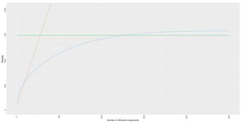
Penalty Regime 1: $P_1(j)=a\left(pv+2\sqrt{pv\psi }+2\psi \right)$, corresponding to setting ${\beta }_j=0$ for $1\le j\le p$ and $\alpha =a\left(pv+2\sqrt{pv\psi }+2\psi \right)$.

Under this penalty, we would infer that any detected anomaly region affects all components. This is likely to lead to a lack of power, if we have anomalous regions that only affect a small number of components. For such anomalies, the following is a good alternative as it has a smaller penalty for fitting collective anomalies with few components:

Penalty Regime 2: $P_2(j)=2(1+ϵ)a\psi +2(1+ϵ)aj\hspace{0.17em}\text{log}\hspace{0.17em}(p)$ which corresponds to setting $\alpha =2(1+ϵ)a\psi$ and ${\beta }_j=2(1+ϵ)a\hspace{0.17em}\text{log}\hspace{0.17em}(p)$, for $1\le j\le p$ and $ϵ>0$.

Comparing penalty regime 2 with penalty regime 1, we see that it has a lower penalty for small j, but a much higher penalty for $j\gg \sqrt{p}/\hspace{0.17em}\text{log}\hspace{0.17em}p$. As such it has higher power against collective anomalies affecting few components, but low power if the collective anomalies affect most components.

If $v\le 2$, then the third penalty regime can be derived:

Penalty Regime 3: $P_3(j)=a(2(\psi +\hspace{0.17em}\text{log}\hspace{0.17em}(p))+jv+2p{c}_{j}f(c_j)+$ $2\sqrt{(jv+2p{c}_{j}f(c_j))(\psi +\hspace{0.17em}\text{log}\hspace{0.17em}(p))})$, where f is the PDF of the ${\chi }_v^2$-distribution and c_j is defined via the implicit equation $\mathbb{P}({\chi }_v^2>c_j)=j/p$.

As can be seen from Figure 2 for the special case of ${\chi }_1^2$-distributed savings, this penalty regime provides a good alternative to the other penalty regimes, with lower penalties for intermediate values of $\left|\mathit{J}\right|$.

All these regimes control the false positive rate, as shown in the following proposition.

Proposition 1.

Assume that there are no collective anomalies. Assume also that the savings $S_i(s,e)$ are independent across components and each stochastically bounded by $a{\chi }_v^2$ for $1\le i\le p$ and let $\widehat{K}$ denote the number of inferred collective anomalies. If we use penalty regime 1 or 2, or if $v\le 2$ and we use penalty regime 3, then, there exists a global constant A such that $\mathbb{P}\{\widehat{K}=0\}\ge 1-A{n}^2{e}^{-\psi }$.

Rather than choosing one penalty regime, we can maximize power against both sparse, intermediate and dense anomalies, by choosing $\alpha ,{\beta }_1,\dots ,{\beta }_p$ so that the resulting penalty function P(j), is the point-wise minimum of the penalty functions $P_1(j),P_2(j)$, and, if available, $P_3(j)$. We call this the composite regime. It is a corollary from Proposition 1, that this composite penalty regime achieves $\mathbb{P}\{\widehat{K}=0\}\ge 1-3A{n}^2{e}^{-\psi }$ for the same global constant A as in Proposition 1, when $S_i(s,e)$ is stochastically bounded by $a{\chi }_v^2$.

2.3 Results on Power

For the case of a collective anomaly characterized by changes in the mean in a subset of the data’s components, we can compare the power of our penalized saving statistic with established results regarding the optimal power of tests. Specifically, we examine behavior under a large p regime. We follow the asymptotic parameterization of Jeng, Cai, and Li (2012) and therefore assume that the collective anomaly is of the form(4) $$\begin{array}{c}{\mathbf{x}}_t^{(i)}=v^{(i)}\mu +{\mathit{\eta }}_t^{(i)},\\ v^{(i)}\sim \{\begin{array}{cc}0\hfill & \text{with}\mathrm{ }\text{prob}.1-p^{-\xi },\hfill \\ 1\hfill & \text{with}\mathrm{ }\text{prob}.p^{-\xi },\hfill \end{array}\mathrm{\hspace{1em}}\mathrm{\hspace{1em}}\text{and}\\ {\mathit{\eta }}_t^{(i)}\stackrel{i.i.d.}{\sim }N(0,1),\mathrm{\hspace{1em}}\mathrm{\hspace{1em}}\text{for}\hspace{1em}s<t\le e,\end{array}$$(4) with the noise ${\mathit{\eta }}_t^{(1)},\dots ,{\mathit{\eta }}_t^{(p)}$ of the different series being independent.

Typically (Jeng, Cai, and Li 2012), changes are characterized as either sparse or dense. In a sparse change, only a few components are affected. Such changes can be detected based on the saving of those few components being larger than expected after accounting for multiple testing. The affected components therefore have to experience strong changes to be reliably detectable. On the other hand, a dense change is a change in which a large proportion of components exhibits anomalous behavior. A well-defined boundary between the two cases exists with $\xi \le \frac{1}{2}$ corresponding to dense and $\xi >\frac{1}{2}$ corresponding to sparse changes (Jeng, Cai, and Li 2012; Enikeeva and Harchaoui 2019). Depending on the setting, the change in mean is parameterized by $r_p\in \mathbb{R}$ in the following manner:$$(e-s){\mu }^2=\{\begin{array}{cc}2r_p\hspace{0.17em}\text{log}\hspace{0.17em}(p)\hfill & \frac{1}{2}<\xi <1,\hfill \\ p^{-2r_p}\hfill & 0\le \xi \le \frac{1}{2}.\hfill \end{array}$$

Both Jeng, Cai, and Li (2012) and Cai, Jeng, and Jin (2011) derived detection boundaries for r_p , separating changes that are too weak to be detected from those changes strong enough to be detected. For the case in which the standard deviation in the anomalous segment is the same as the typical standard deviation, the detectability boundaries correspond to ${\rho }^{-}={(1-\sqrt{1-\xi })}^2$ if $3/4<\xi <1,{\rho }^{-}=\xi -1/2$ if $1/2<\xi \le 3/4$ for the sparse case; and ${\rho }^{+}=(1/2-\xi )/2$ for the dense case ($0\le \xi \le \frac{1}{2}$). The following proposition establishes that the penalized saving statistic has power against all sparse changes within the detection boundary, as well as against dense changes within the detection boundary

Proposition 2.

Let the typical mean be known and the series ${\mathbf{x}}_1,\dots ,{\mathbf{x}}_n$ contain an anomalous segment ${\mathbf{x}}_{s+1},\dots ,{\mathbf{x}}_e$, which follows the model specified in Equation (4)(4) $$\begin{array}{c}{\mathbf{x}}_t^{(i)}=v^{(i)}\mu +{\mathit{\eta }}_t^{(i)},\\ v^{(i)}\sim \{\begin{array}{cc}0\hfill & \text{with}\mathrm{ }\text{prob}.1-p^{-\xi },\hfill \\ 1\hfill & \text{with}\mathrm{ }\text{prob}.p^{-\xi },\hfill \end{array}\mathrm{\hspace{1em}}\mathrm{\hspace{1em}}\text{and}\\ {\mathit{\eta }}_t^{(i)}\stackrel{i.i.d.}{\sim }N(0,1),\mathrm{\hspace{1em}}\mathrm{\hspace{1em}}\text{for}\hspace{1em}s<t\le e,\end{array}$$(4) . Let $r_p>{\rho }^{-}$ if $\frac{1}{2}<\xi <1$ or $r_p<{\rho }^{+}$ if $0\le \xi \le \frac{1}{2}$. Then the number of collective anomalies, $\widehat{K}$, estimated by MVCAPA using the composite penalty with a = 1, v = 1 and $\psi (p,n)=2\hspace{0.17em}\text{log}\hspace{0.17em}(n)+2\hspace{0.17em}\text{log}\hspace{0.17em}(\hspace{0.17em}\text{log}\hspace{0.17em}(p))$ on the data ${\mathbf{x}}_1,\dots ,{\mathbf{x}}_n$, satisfies$$\mathbb{P}\left(\widehat{K}\ne 0\right)\to 1\text{as}p\to \infty$$provided that $\text{log}\hspace{0.17em}(n)=o(\hspace{0.17em}\text{log}\hspace{0.17em}(p))$.

Rather than requiring μ_i to be 0, or a common value μ, it is trivial to extend the result to the case where ${\mu }_1,\dots ,{\mu }_p$ are iid random variables whose magnitude exceeds μ with probability $p^{-\xi }$. It is worth noticing that the third penalty regime is required to obtain optimal power against the intermediate sparse setting $\frac{1}{2}<\xi \le \frac{3}{4}$.

3 Inference for Multiple Anomalies

A natural way of extending the methodology introduced in Section 2 to infer multiple collective anomalies, is to maximize the penalized saving jointly over the number and location of potentially multiple anomalous windows. That is we infer $\widehat{K},({\widehat{s}}_1,{\widehat{e}}_1,{\widehat{\mathit{J}}}_1)$,…, $({\widehat{s}}_{\widehat{K}},{\widehat{e}}_{\widehat{K}},{\widehat{\mathit{J}}}_{\widehat{K}})$ by directly maximizing(5) $$\sum _{k=1}^{\widehat{K}}\mathcal{S}\left({\widehat{s}}_k,{\widehat{e}}_k\right),$$(5) subject to ${\widehat{e}}_k-{\widehat{s}}_k\ge l$ and ${\widehat{e}}_k\le {\widehat{s}}_{k+1}$.

Such an approach may not be robust to point outliers, which could either be incorrectly inferred as anomalous segments or cause anomalous segments to be broken up, thus limiting interpretability. The occurrence of both these problems can be prevented by using bounded cost functions (Fearnhead and Rigaill 2019). For example, when looking for changes in mean using a square error loss function, we truncate the loss at a value $\beta \prime$ to obtain the cost $\mathcal{C}(x,\mu )=\min (\beta \prime ,{(x-\mu )}^2/{\sigma }^2)$, which is equivalent to using Tukey’s biweight loss.

When only spurious detection of anomalous regions due to point outliers is to be avoided, just the cost used for the typical segments has to be truncated. To do this we define $\mathcal{S}\prime ({\mathbf{x}}_t)$ to be the reduction in cost obtained by truncating the cost of a subset of the components of the observation ${\mathbf{x}}_t^{(i)}$. For example, if our anomalies correspond to changes in mean and we are using square error loss, or equivalently the Gaussian log-likelihood-based cost, then$$\mathcal{S}\prime \left({\mathbf{x}}_t\right)=\sum _{i=1}^p\max \left({\left(\frac{{\mathbf{x}}_t^{(i)}-{\mathit{\mu }}_0^{(i)}}{{\mathit{\sigma }}_0^{(i)}}\right)}^2-\beta \prime ,0\right),$$where as before ${\mathit{\mu }}_0^{(i)}$ and ${\mathit{\sigma }}_0^{(i)}$ are the mean and standard deviation of normal data for component i. Joint inference on collective and point anomalies is then performed by maximizing(6) $$\sum _{k=1}^{\widehat{K}}\mathcal{S}\left({\widehat{s}}_k,{\widehat{e}}_k\right)+\sum _{t\in O}\mathcal{S}\prime \left({\mathbf{x}}_t\right),$$(6) with respect to $\widehat{K},({\widehat{s}}_1,{\widehat{e}}_1,{\widehat{\mathit{J}}}_1)$,…, $({\widehat{s}}_{\widehat{K}},{\widehat{e}}_{\widehat{K}},{\widehat{\mathit{J}}}_{\widehat{K}})$, and the set of point anomalies O, subject to ${\widehat{e}}_k-{\widehat{s}}_k\ge l,{\widehat{e}}_k<{\widehat{s}}_{k+1}$ $({\cup }_i[s_i+1,e_i])\cap O=\varnothing$.

Similarly, setting the cost $\mathcal{C}()$ of collective anomalies to the truncated loss prevents collective anomalies from being split up by point anomalies. This has been implemented for anomalies characterized by a change in mean, using Tukey’s bi-weight loss, in the anomaly package.

The threshold $\beta \prime$ has to be chosen depending on whether it is of interest to detect point anomalies as such. When this is not the case, $\beta \prime$ tunes the robustness of the approach—the lower it is, the more robust the approach becomes to outliers, whilst higher values of $\beta \prime$ lead to more power. When point anomalies are of interest, $\beta \prime$ can be chosen with the aim of controlling false positives under the null hypothesis of no point anomalies. When Tukey’s biweight loss is used, the following proposition holds for any penalty $\beta \prime$:

Proposition 3.

Let $x_1^{(i)},\dots ,x_n^{(i)}$ be iid sub-Gaussian(λ) with known mean μ_i . Let the series be independent for $1\le i\le p$. Let $\widehat{O}$ denote the set of point anomalies inferred by MVCAPA using cost $\mathcal{C}(x,\mu )=\min (\beta \prime ,{(x-\mu )}^2)$. Then, there exists a global constant $A\prime$ such that$$\mathbb{P}\left(\widehat{O}=\varnothing \right)\ge 1-A\prime np{e}^{-\frac{1}{2\lambda }\beta \prime }.$$

This suggests setting $\beta \prime =2\lambda \hspace{0.17em}\text{log}\hspace{0.17em}(p)+2\lambda \psi$, where ψ is as in Section 2.2.

4 Computation

The standard approach to extend a method for detecting an anomalous window to detecting multiple anomalous windows is through circular binary segmentation (CBS; Olshen et al. 2004)—which repeatedly applies the method for detecting a single anomalous window or point anomaly. Such an approach is equivalent to using a greedy algorithm to approximately maximize the penalized saving and has computational cost of O(Mn), where M is the maximal length of collective anomalies and n is the number of observations. Consequently, the runtime of CBS is $O(n^2)$ if no restriction is placed on the length of collective anomalies. We will show in this section that we can directly maximize the penalized saving by using a pruned dynamic programme. This enables us to jointly estimate the anomalous windows, at the same or at a lower computational cost than CBS.

We will focus on the optimization of the criteria that incorporates point anomalies (6), though a similar approach applies to optimizing (5). Writing S(m) for the largest penalized saving of all observations up to and including time m, it is straightforward to derive the recursion.$$S(m)=\max \mathrm{}(\mathrm{}S(m-1)+\mathcal{S}\prime \left({\mathbf{x}}_m\right),\underset{{}_{0\le t\le m-l}}{\max }\mathrm{}(\mathrm{}S(t)+\mathcal{S}\left(t,m\right)\mathrm{})\mathrm{})$$with $S(0)=0$. Calculating $\mathcal{S}(t,m)$ is, on average, an $O(p\hspace{0.17em}\text{log}\hspace{0.17em}(p))$ operation, since it requires sorting the savings made from introducing a change in each component. This sorting is not required if the ${\beta }_i$ are identical, whence the computational cost to O(p). For a maximum segment length M, the computational cost of the dynamic programme is O(Mn).

If no maximum segment length is specified, then the computational cost scales quadratically in n. However, the solution space of the dynamic programme can be pruned in a fashion similar to Killick, Fearnhead, and Eckley (2012) and Fisch, Eckley, and Fearnhead (2018) to reduce this computational cost. This is discussed in Section 1.1 of the supplementary material. As a result of this pruning, we found the runtime of MVCAPA to be close to linear in n, when the number of collective anomalies increased linearly with n; see Section 7.3.

5 Accuracy of Detecting Multiple Anomalies

While we have shown that MVCAPA has good properties when detecting a single anomalous window for the change in mean setting, it is natural to ask whether the extension to detecting multiple anomalous windows will be able to consistently infer the number of anomalous windows and accurately estimate their locations. Specifically, we will be considering the case of joint detection of sparse and dense collective anomalies in mean. Developing such results is notoriously challenging, as can be seen from the fact that previous work on this problem (Jeng, Cai, and Li 2012) has not provided any such results. Our novel combinatorial arguments can be applied to other settings (e.g., mean and variance) within the penalized cost framework.

Consider a multivariate sequence ${\mathbf{x}}_1,\dots ,{\mathbf{x}}_n\in {\mathbb{R}}^p$, which is of the form ${\mathbf{x}}_t=\mathit{\mu }(t)+{\mathit{\eta }}_t,$ where the mean $\mathit{\mu }(t)$ follows a subset multivariate epidemic changepoint model with K epidemic changepoints in mean. For simplicity, we assume that within an anomalous window all affected components experience the same change in mean, and that the noise process is iid Gaussian, that is, that for each component i,(7) $${\mathit{\mu }}^{(i)}(t)={\mathit{\mu }}_k\text{if}{s}_k<t\le e_k\text{and}i\in {\mathbf{J}}_k$$(7) and 0 otherwise.

Consider also the following choice of penalty:(8) $$\sum _{i=1}^j{\mathit{\beta }}_i=\{\begin{array}{cc}C\psi +Cj\hspace{0.17em}\text{log}\hspace{0.17em}(p)\hfill & \text{if}j\le k^{*},\hfill \\ p+C\psi +C\sqrt{p\psi }\hfill & \text{if}j>k^{*}.\hfill \end{array}$$(8)

Here, C is a constant, $\psi :=\psi (n,p)$ sets the rate of convergence and the threshold$$k^{*}=p^{1/2}\frac{\psi }{\hspace{0.17em}\text{log}\hspace{0.17em}(p)},$$is defined as the threshold separating sparse changes from dense changes. This penalty regime is identical, up to $O(ϵ)$, to the point-wise minimum between penalty regimes 1 and 2, when $C=2+ϵ$.

Anomalous regions can be easier or harder to detect depending on the strength of the change in mean characterizing them and the number of components ($\left|{\mathbf{J}}_k\right|$ for the kth anomaly) they affect. This intuition can be quantified by$${△}_k^2=\{\begin{array}{cc}\frac{{\mathit{\mu }}_k^2}{\hspace{0.17em}\text{log}\hspace{0.17em}(p)+\psi |{\mathbf{J}}_k{|}^{-1}}\hfill & \text{if}\left|{\mathbf{J}}_k\right|\le k^{*},\hfill \\ \frac{{\mathit{\mu }}_k^2}{\sqrt{p\psi }|{\mathbf{J}}_k{|}^{-1}+\psi |{\mathbf{J}}_k{|}^{-1}}\hfill & \text{if}\left|{\mathbf{J}}_k\right|>k^{*},\hfill \end{array}$$

which we define to be the signal strength of the kth anomalous region. The following consistency result then holds

Theorem 1.

Let the typical means be known. There exists global constants A and C₀ such that for all $C\ge C_0$ the inferred partition $\tau =\{({\widehat{s}}_1,{\widehat{e}}_1,{\widehat{\mathbf{J}}}_1),\dots ,({\widehat{s}}_{\widehat{K}},{\widehat{e}}_{\widehat{K}},{\widehat{\mathbf{J}}}_{\widehat{K}})\}$ obtained by applying MVCAPA using the penalty regime specified in Equations (8)(8) $$\sum _{i=1}^j{\mathit{\beta }}_i=\{\begin{array}{cc}C\psi +Cj\hspace{0.17em}\text{log}\hspace{0.17em}(p)\hfill & \text{if}j\le k^{*},\hfill \\ p+C\psi +C\sqrt{p\psi }\hfill & \text{if}j>k^{*}.\hfill \end{array}$$(8) and no minimum segment length, on data x which follows the distribution specified in Equations (7)(7) $${\mathit{\mu }}^{(i)}(t)={\mathit{\mu }}_k\text{if}{s}_k<t\le e_k\text{and}i\in {\mathbf{J}}_k$$(7) satisfies(9) $$\begin{array}{c}\mathbb{P}\left(\widehat{K}=K,\hspace{1em}\left|{\widehat{s}}_k-s_k\right|<\frac{10C}{{△}_k^2},\hspace{1em}\left|{\widehat{e}}_k-e_k\right|<\frac{10C}{{△}_k^2}\right)\\ \mathrm{\hspace{1em}}\mathrm{\hspace{1em}}>1-A{n}^3{e}^{-\psi },\end{array}$$(9) provided that, for $k=1,\dots ,K$,$$e_k-s_k\ge \frac{40C}{{△}_k^2},s_{k+1}-e_k\ge \frac{40C}{{△}_k^2},s_k-e_{k-1}\ge \frac{40C}{{△}_k^2}.$$

The result is proved in the supplementary material using combinatorial arguments. This finite sample result holds for a fixed C, which is independent of n, p, K, and/or ${△}_k$.

Theorem 1 can be extended to allow for both a minimum and maximum segment length. The proof of the theorem is based on partitioning all possible segmentations in to one of two classes, corresponding to those which are consistent with the event in the probability statement of Equation (9)(9) $$\begin{array}{c}\mathbb{P}\left(\widehat{K}=K,\hspace{1em}\left|{\widehat{s}}_k-s_k\right|<\frac{10C}{{△}_k^2},\hspace{1em}\left|{\widehat{e}}_k-e_k\right|<\frac{10C}{{△}_k^2}\right)\\ \mathrm{\hspace{1em}}\mathrm{\hspace{1em}}>1-A{n}^3{e}^{-\psi },\end{array}$$(9) and those that are not. The proof then shows that conditional on a different event, whose probability is greater than $1-A{n}^3{e}^{-\psi }$, any segmentation in the latter class will have a lower penalized saving than at least one segmentation in the former class, and thus cannot be optimal under our criteria. This argument still works providing our choice of minimum or maximum segment lengths does not exclude any segmentations from the first class of segmentations, that is, if$$l\le \underset{{}_k}{\min }\left(e_k-s_k-\frac{20C}{{△}_k^2}\right),\hspace{1em}m\ge \underset{{}_k}{\max }\left(e_k-s_k+\frac{20C}{{△}_k^2}\right).$$

6 Incorporating Lags

6.1 Extending the Test Statistic

So far, we have assumed that all anomalous windows are perfectly aligned. In some applications, such as the vibrations recorded by seismographs at different locations, certain components will start exhibiting atypical behavior later and/or return to the typical behavior earlier. The model in Equation (1)(1) $${\mathit{\theta }}^{(i)}(t)={\mathit{\theta }}_k^{(i)}\mathrm{ }\text{if}{s}_k<t\le e_k\text{and}i\in {\mathbf{J}}_k$$(1) can be extended to allow for lags in the start or end of each anomalous window. The parameter ${\mathit{\theta }}^{(i)}(t)$ is then assumed to be(10) $${\mathit{\theta }}^{(i)}(t)={\mathit{\theta }}_k^{(i)}\text{if}{s}_k+{\mathbf{d}}_k^{(i)}<t\le e_k-{\mathbf{f}}_k^{(i)}\text{and}i\in {\mathbf{J}}_k,$$(10) and ${\mathit{\theta }}_0^{(i)}$ otherwise. Here, the start and end lag of the ith component during the kth anomalous window are denoted, respectively, by $0\le {\mathbf{d}}_k^{(i)}\le w$ and $0\le {\mathbf{f}}_k^{(i)}\le w$, for some maximum lag-size, w, and satisfy $s_k+{\mathbf{d}}_k^{(i)}<e_k-{\mathbf{f}}_k^{(i)}$. The remaining notation is as before.

The statistic introduced in Section 2 can easily be extended to incorporate lags. The only modification this requires is to redefine the saving ${\mathcal{S}}_i(s,e)$ to be(11) $$\begin{array}{c}{\max }_{\stackrel{0\le {\mathbf{d}}^{(i)},{\mathbf{f}}^{(i)}\le w}{e¯s¯{\mathbf{d}}^{(i)}¯{\mathbf{f}}^{(i)}\ge l}}[{\mathcal{C}}_i\left({\mathbf{x}}_{(s+1+{\mathbf{d}}^{(i)}):(e-{\mathbf{f}}^{(i)})}^{(i)},{\mathit{\theta }}_0^{(i)}\right)\hfill \\ -{\min }_{\mathit{\theta }}\left({\mathcal{C}}_i\left({\mathbf{x}}_{(s+1+{\mathbf{d}}^{(i)}):(e-{\mathbf{f}}^{(i)})}^{(i)},\mathit{\theta }\right)\right)],\hfill \end{array}$$(11)

where w is the maximal allowed lag. We then infer O, $\widehat{K},({\widehat{s}}_1,{\widehat{e}}_1,{\widehat{\mathbf{d}}}_1,{\widehat{\mathbf{f}}}_1,{\widehat{\mathit{J}}}_1)$,…, $({\widehat{s}}_{\widehat{K}},{\widehat{e}}_{\widehat{K}},{\widehat{\mathbf{d}}}_{\widehat{K}},{\widehat{\mathbf{f}}}_{\widehat{K}},{\widehat{\mathit{J}}}_{\widehat{K}})$ by directly maximizing the penalized saving(12) $$\sum _{k=1}^{\widehat{K}}\mathcal{S}\left({\widehat{s}}_k,{\widehat{e}}_k\right)+\sum _{t\in O}\mathcal{S}\prime \left({\mathbf{x}}_t\right),$$(12) with respect to $\widehat{K},({\widehat{s}}_1,{\widehat{e}}_1,{\widehat{\mathbf{d}}}_1,{\widehat{\mathbf{f}}}_1,{\widehat{\mathit{J}}}_1)$,…, $({\widehat{s}}_{\widehat{K}},{\widehat{e}}_{\widehat{K}},{\widehat{\mathbf{d}}}_K,{\widehat{\mathbf{f}}}_K,{\widehat{\mathit{J}}}_{\widehat{K}})$, and the set of point anomalies O, subject to $0\le {\widehat{\mathbf{d}}}_k,{\widehat{\mathbf{f}}}_k\le w,({\widehat{e}}_k-{\widehat{\mathbf{f}}}_k)-({\widehat{s}}_k+{\widehat{\mathbf{d}}}_k)\ge l$ and ${\widehat{e}}_k<{\widehat{s}}_{k+1}$.

Introducing lags means searching over more possible start and end points for the anomalous segments in each series. Consequently, increased penalties are required to control the false error rate. A simple general way of doing is based on a Bonferonni correction to allow for the different start and end-points of anomalies in different series. It is shown in Section 1.2 of the supplementary material that if we use the penalty regimes from Section 2.2 but inflate ψ by adding $4\hspace{0.17em}\text{log}\hspace{0.17em}(w+1)$ we obtain the same bound on false positives.

When anomalies correspond to a change in mean in Gaussian data, we show in Section 2.6 of the supplementary material that we can improve on this and use the following weaker penalty and still control the false positive probability.

Penalty Regime 2’: $P_2^{\prime }(j)=2(1+ϵ)\psi +2(1+ϵ)j\hspace{0.17em}\text{log}\hspace{0.17em}(p)+2(1+ϵ)j\hspace{0.17em}\text{log}\hspace{0.17em}(w+1)$ corresponding to $\alpha =2(1+ϵ)\psi$ and ${\beta }_j=2(1+ϵ)\hspace{0.17em}\text{log}\hspace{0.17em}(p)+2(1+ϵ)\hspace{0.17em}\text{log}\hspace{0.17em}(w+1)$, for $1\le j\le p$.

An important question is how to choose the maximum lag length, w. In practice this needs to be guided by the application, and any knowledge about the degree to which common anomalies may be misaligned. In Section 2.6 in the Supplementary Material we provide theory which shows the gain in power that can be achieved by incorporating lags when collective anomalies are misaligned. However, too large a value of w may lead to a loss of power due to the inflation of the penalties that are needed, or, in extreme cases, may mean that separate anomalies are fit as a single misaligned anomaly. We investigate the choice of w empirically in Section 7.

6.2 Computational Considerations

The dynamic programming approach described in Section 4 can also be used to minimize the penalized negative saving in Equation (12)(12) $$\sum _{k=1}^{\widehat{K}}\mathcal{S}\left({\widehat{s}}_k,{\widehat{e}}_k\right)+\sum _{t\in O}\mathcal{S}\prime \left({\mathbf{x}}_t\right),$$(12) . Solving the dynamic programme requires the computation of ${\mathcal{S}}_i(t,m)$ for $1\le i\le p$ for all permissible t at each step of the dynamic programme. Computing these savings ex nihilo every time leads to the computational cost of the dynamic programme to scale quadratically in $(w+1)$.

However, it is possible to reduce the computational cost of including lags by storing the savings$${\mathcal{C}}_i\left({\mathbf{x}}_{(a+1):b}^{(i)},{\mathit{\theta }}_0^{(i)}\right)-\underset{{}_{\theta }}{\min }\left[{\mathcal{C}}_i\left({\mathbf{x}}_{(a+1):b}^{(i)},\mathit{\theta }\right)\right]$$for $t-w\le b\le t$ and $0\le a\le b-l$. These can then be updated in each step of the dynamic programme at a cost of at most O(np). From these, it is possible to calculate all ${\mathcal{S}}_i(t,m)$ required for a step of the dynamic programme in just $O(np(w+1))$ comparisons. This reduces the computational cost of each step of the dynamic programme to $O(pn(w+1)+pn\hspace{0.17em}\text{log}\hspace{0.17em}(p))$. Crucially, only the comparatively cheap operations of allocating memory and finding the maximum of two numbers increase with w + 1. Furthermore, it is possible to adapt the pruning rule for the dynamic programme to incorporate lags. The details for this and full pseudocode can be found in the supplementary material.

7 Simulation Study

We now compare the performance of MVCAPA to that of other popular methods. In particular, we compare detection accuracy, precision, as well as the runtime with PASS (Jeng, Cai, and Li 2012) and Inspect (Wang and Samworth 2018, 2016). PASS (Jeng, Cai, and Li 2012) uses higher criticism in conjunction with circular binary segmentation (Olshen et al. 2004) to detect subset multivariate epidemic changepoints. Inspect (Wang and Samworth 2018) uses projections to find sparse classical changepoints and therefore provides a benchmark for the detection approach consisting of modeling epidemic changes as two classical changepoints. For the purpose of this simulation study, we used the implementation of PASS available on the author’s website and the Inspect implementation from the R package InspectChangepoint.

The comparison was carried out on simulated multivariate time series with n = 5000 observations for p components with iid N(0, 1) noise, AR(1) noise ($\rho =0.3$), or t₁₀-distributed noise for a range of values of p. To these, collective anomalies affecting k components occurring at a geometric rate of 0.001 (leading to an average of about 5 collective anomalies per series) were added. The lengths of these collective anomalies are iid Poisson-distributed with mean 20. Within a collective anomaly, the start and end lags of each component are drawn uniformly from the set $\{0,\dots ,w\}$, subject to their sum being less than the length of the collective anomaly. Note that w = 0 implies the absence of lags. The means of the components during the collective anomaly are drawn from an $N(0,{\sigma }^2)$-distribution. In particular, we considered the following cases, emulating different detectable regimes introduced in Section 2.3.

1. The most sparse regime possible: a single component affected by a strong anomaly without lags, that is, $\sigma =2\hspace{0.17em}\text{log}\hspace{0.17em}(p)$, w = 0, and k = 1.

2. The most dense regime possible: all components affected by weak anomalies without lags, that is, $\sigma =p^{-1/4}$, w = 0, and k = p.

3. A regime close to the boundary between sparse and dense changes, that is, k = 2 when p = 10 and k = 6 when p = 100 with $\sigma =\hspace{0.17em}\text{log}\hspace{0.17em}(p)$ and w = 0.

4. A regime close to the boundary between sparse and dense changes, but with lagged collective anomalies, that is, the same as 3 but with w = 10.

This analysis was repeated with 5-point anomalies distributed $N(0,8\hspace{0.17em}\text{log}\hspace{0.17em}(p))$. The $\text{log}\hspace{0.17em}(p)$-scaling of the variance ensures that the point anomalies are anomalous even after correcting for multiple testing over the p different components.

7.1 Detection Accuracy

All methods are sensitive to the choice of a threshold parameter that defines how much evidence of an anomaly or change there needs to be before one is flagged. To make our results robust to this choice, we investigate how each method performs as we vary its threshold parameter, and plot the proportion of anomalies detected against the number of false positives. The curves were obtained over 1000 simulated datasets. For MVCAPA, we typically set w = 0, but also tried w = 10 and w = 20 for the third and fourth setting. The median and median absolute deviation were used to robustly estimate the mean and variance. Throughout the experiments, for MVCAPA, we used the composite penalty regime for w = 0 and penalty regime 2’ for w > 0, and varied its threshold by rescaling the penalty by a constant that is varied. We also set the maximum segment lengths for both MVCAPA and PASS to 100 and the minimum segment length of MVCAPA to 2. The α₀ parameter of PASS, which excludes the ${\alpha }_0-1$ lowest p-values from the higher criticism statistic to obtain a better finite sample performance (see Jeng, Cai, and Li 2012) was set to k or 5, whichever was the smallest. For MVCAPA and PASS, we considered a detected segment to be a true positive if its start and end point both lie within 20 observations of that of a true collective anomalies’ start and end point respectively. For Inspect, we considered a detected change to be a true positive if it was within 20 observation of a true start or end point. When point anomalies were added to the data, we considered segments of length one returned by PASS to be point anomalies. Qualitatively similar results were obtained as we vary the definition of a true positive: see Figure 8 the supplementary material.

A subset of the results for three of the settings considered can be found in Figure 3. The full results for the four settings can be found in Figures 2 to 5 of the Supplementary Material. We can see that Inspect usually does worst. This is especially true when changes become dense, which is no surprise given the method was introduced to detect sparse changes. However it is also the case for very sparse changes—the setting for which Inspect has been designed, highlighting the advantage of treating epidemic changes as such. We additionally see that MVCAPA generally outperforms PASS. This advantage is particularly pronounced in the case in which exactly one component changes. This is a setting which PASS has difficulties dealing with due to the convergence properties of the higher criticism statistic at the lower tail (Jeng, Cai, and Li 2012). PASS outperformed MVCAPA in the second setting for p = 10, when it was assisted by a large value of α₀, which considerably reduced the number of candidate collective anomalies it had to consider.

Fig. 3 Proportion of anomalies detected against the ratio of false positives to true positives for setting 1, 3, and 4 (top row to bottom row). MVCAPA is in black, PASS in green, and Inspect in red. The solid black line corresponds to w = 0, the dashed one to w = 10 and the dotted one to w = 20. The x-axis denotes the number of false discoveries normalized by the total number of real anomalies present in the data.

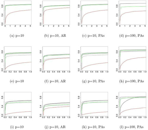
Figure 3(a) and (b) shows that MVCAPA performs best when the correct maximal lag is specified. They also demonstrate that specifying a lag and therefore overestimating the lag when no lag is present adversely affects performance of MVCAPA. However, when lags are present, over-estimating the maximal lag appears preferable to underestimating it. Finally, the comparison between Figures 3(b) and 3(c) shows that the performance of MVCAPA is hardly affected by the presence of point anomalies.

We have also considered the case in which collective anomalies are characterized by joint changes in mean and variance. Detection accuracy plots for that setting can be found in Figures 6 and 7 in the supplementary material.

7.2 Precision

We compared the precision of the three methods by measuring the accuracy (in mean absolute distance) of true positives. Only true positives detected by all methods were taken into account to avoid selection bias. We used the default parameters for MVCAPA and PASS, whilst we set the threshold for Inspect to a value leading to comparable number of true and false positives. To ensure a suitable number of true positives for Inspect we doubled σ in the second scenario. The results of this analysis can be found in Table 1 and show that MVCAPA is usually the most precise approach, exhibiting a significant gain in accuracy against PASS. Whilst we noted that erring on specifying too large a maximal lag was better in terms of power of the MVCAPA to detect collective anomalies, we see that it does have an adverse impact on the accuracy of their estimated locations.

Table 1 Precision of true positives detected by all methods measured in mean absolute distance for MVCAPA, PASS, and Inspect.

Setting	p	Lag	PAs.	MVCAPA	MVCAPA, w = 10	MVCAPA, w = 20	Inspect	PASS
1	10	0	–	0.09	–	–	0.64	0.31
1	100	0	–	0.02	–	–	0.40	0.62
1	10	0	✓	0.09	–	–	0.62	0.38
1	100	0	✓	0.03	–	–	0.40	0.67
2	10	0	–	0.09	–	–	0.74	0.52
2	100	0	–	0.01	–	–	0.71	0.54
2	10	0	✓	0.05	–	–	0.69	0.46
2	100	0	✓	0.01	–	–	0.67	0.51
3	10	0	–	0.11	2.31	3.30	0.72	0.27
3	100	0	–	0.01	3.43	3.83	0.53	0.29
3	10	0	✓	0.09	2.23	3.26	0.69	0.22
3	100	0	✓	0.01	3.35	3.82	0.53	0.23
4	10	10	–	0.63	0.46	1.09	0.80	2.53
4	100	10	–	1.27	0.18	1.57	0.61	3.64
4	10	10	✓	0.72	0.51	1.22	0.83	2.60
4	100	10	✓	1.23	0.21	1.58	0.59	3.77

7.3 Runtime

We compared the scaling of the runtime of MVCAPA, PASS, and Inspect in both the number of observations n, as well as the number of components p. To evaluate the scaling in n we set p = 10 and varied n on data without any anomalies. We repeated this analysis with collective anomalies appearing (on average) every 100 observations. The results of these two analyses can be found in Figures 4(a) and (b), respectively. We note that the slope of MVCAPA is very close to 2, in the anomaly-free setting and very close to 1 in the setting in which the number of anomalies increases linearly with the number of observations, suggesting quadratic and linear behavior, respectively, whilst the slopes of PASS and Inspect are close to 2 and 1 respectively in both cases.

Fig. 4 A comparison of run-times for MVCAPA (red squared), PASS (green circles), and Inspect (blue triangles). Robust lines of best fit have been added. All logarithms are in base 2. Left-hand and middle plots are for p = 10 and varying n for data with, respectively, no collective anomalies and a collective anomaly every 100 observations on average. Right-hand plot is for n = 100 and varying p.

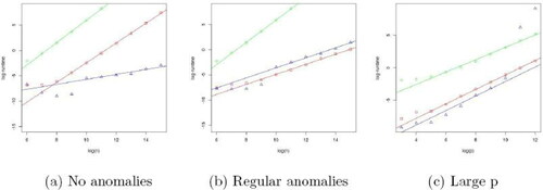
Turning to the scaling of the three methods in p, we set n = 100 and varied p. The results of this analysis can be found in Figure 4(c). We note that the slopes of all methods are close to 1 suggesting linear behavior. However, Inspect becomes very slow once p exceeds a certain threshold.

8 Detecting Copy Number Variation

We now apply MVCAPA to extract copy number variations (CNVs) from genetics data. The data consists of a log-R ratio between observed and expected intensity (defined in Lin, Naj and Wang 2013) evaluated along the genome. The typical mean of this statistics is therefore equal to 0, whilst deviations from 0 correspond to CNVs. A multivariate approach to detecting CNVs is attractive because they are often shared across individuals. By borrowing signal across individuals we should gain power for detecting CNVs which have a weak signal. However, as we will become apparent from our results, shared variations do not always align perfectly across individuals.

In this section, we reuse the design of Bardwell and Fearnhead (2017) to compare MVCAPA with PASS. We investigate the performance of both methods on two chromosomes (Chromosome 16 with $n=59,590$ measurements and Chromosome 6 with $n=126,695$ measurements) over 18 individuals, which we split into 3 folds of p = 6 individuals. We set the maximum segment length for MVCAPA and PASS to 100. To investigate the potential benefit of allowing for lags, we repeated the experiment for MVCAPA both with w = 0 (i.e., not allowing for lags) and w = 40. Since $n\gg p$ in this application, we used the sparse penalty setting (Regime 2) for MVCAPA.

Whilst the exact ground truth is unknown, we can compare methods by how accurately they detect known CNVs for a given test size. We used known CNVs from the HapMap project (International HapMap Consortium 2003) as true positives and tuned the penalties and thresholds so that 4% of the genome was flagged as anomalous for all methods.

The results of this analysis on Chromosome 16 can be found in Table 2 while the results for Chromosome 6 can be found in Table 10 in the supplementary material. These tables show that MVCAPA shows much more consistency across folds than PASS. We also see that allowing for lags generally led to a better performance, thus suggesting nonperfect alignment of CNVs across individuals. Moreover, MVCAPA was very fast taking 5 seconds to analyze the longer genome on a standard laptop when we did not allow lags, and 10 seconds when we allowed for lags. The R implementation of PASS took 17 min.

Table 2 A comparison between PASS, MVCAPA without lags, and MVCAPA with a lag of up to 40 for chromosome 16.

Truth	PASS			MVCAPA (w = 40)			MVCAPA (w = 0)
Start	Rep 1	Rep 2	Rep 3	Rep 1	Rep 2	Rep 3	Rep 1	Rep 2	Rep 3
2619669		✓
2638575		✓
21422575	✓	✓	✓	✓	✓	✓	✓	✓	✓
32165010	✓	✓	✓	✓	✓	✓	✓	✓	✓
34328205	✓	✓		✓	✓	✓	✓	✓	✓
54351338	✓	✓	✓	✓	✓	✓
70644511				✓	✓	✓	✓	✓	✓

NOTES: Each row represents a known copy number variation, their starting point (as defined by the HapMap) being indicated in the first column. Successful detections are indicated by ticks.

9 Discussion

Although we have focused on anomalies that relate to changes in mean, by choosing a cost based on an appropriate model the framework can be applied to detecting a variety of types of change. Moreover, one can use different likelihood-based costs for different components and thus detect collective anomalies for data with a mix of data types. It is also possible to use a similar penalized cost to detect changepoints in multivariate data, and this extension has been considered in Tickle, Eckley, and Fearnhead (2021).

We have presented theory that indicates how to choose appropriate penalties for the method. However, this theory relies on various assumptions, for example that the data are independent across series and across time. Results for other penalized cost procedures (Lavielle and Moulines 2000) suggest that one way of accounting for these assumptions not holding is to increase the penalties. We suggest doing this by taking the penalties suggested by theory and scaling them all by a constant. The choice of constant can be made in a data-driven way through analysis of performance on test data (Hocking et al. 2013), or by comparing changes the fit as we vary the constant (Haynes, Eckley, and Fearnhead 2017). Alternatively, we can model the dependencies, see Tveten, Eckley, and Fearnhead (2020) for an extension of MVCAPA to allow for correlation in the data across components.

MVCAPA does not quantify uncertainty about estimates of individual collective anomalies. This is similar to other epidemic changepoint and changepoint methods that output a single estimate of their locations. Recent work (Hyun et al. 2021; Jewell, Fearnhead, and Witten 2019) has shown how to obtain valid p-values that quantify the uncertainty that each estimated change is close to an actual change; the output of these methods can then be used to give, for example, control of the false discovery rate for the estimated changes. These ideas should be able to be extended to cover the collective anomaly problem, and hence quantify uncertainty of each collective anomaly detected by MVCAPA.

Supplementary Material

The supplementary material contains a pdf with proofs, additional results from the simulation study and data analysis, and further algorithmic details for MVCAPA. It also contains example R code from the simulation study.

Additional information

Funding

This work was supported by EPSRC grant numbers EP/N031938/1 (StatScale) and EP/L015692/1 (STOR-i). The authors also acknowledge British Telecommunications plc (BT) for financial support, David Yearling and Kjeld Jensen in BT Research & Innovation for discussions. Thanks also to Lawrence Bardwell for providing us with data and code reproducing results from his article.

References

- Bardwell, L., and Fearnhead, P. (2017), “Bayesian Detection of Abnormal Segments in Multiple Time Series,” Bayesian Analysis, 12, 193–218. DOI: https://doi.org/10.1214/16-BA998.
- Cai, T., Jeng, J., and Jin, J. (2011), “Optimal Detection of Heterogeneous and Heteroscedastic Mixtures,” Journal of the Royal Statistical Society, 73, Series B, 629–662.
- Chandola, V., Banerjee, A., and Kumar, V. (2009), “Anomaly Detection: A Survey,” ACM Computing Surveys, 41, 15. DOI: https://doi.org/10.1145/1541880.1541882.
- Cho, H., and Fryzlewicz, P. (2015), “Multiple-Change-Point Detection for High Dimensional Time Series Via Sparsified Binary Segmentation,” Journal of the Royal Statistical Society, Series B, 77, 475–507. DOI: https://doi.org/10.1111/rssb.12079.
- Cui, Y., Bangalore, P., and Tjernberg, L. B. (2018), “An Anomaly Detection Approach Based on Machine Learning and Scada Data for Condition Monitoring of Wind Turbines,” in 2018 IEEE International Conference on Probabilistic Methods Applied to Power Systems (PMAPS), IEEE, pp. 1–6. DOI: https://doi.org/10.1109/PMAPS.2018.8440525.
- Davis, R. A., Lee, T. C. M., and Rodriguez-Yam, G. A. (2006), “Structural Break Estimation for Nonstationary Time Series Models,” Journal of the American Statistical Association, 101, 223–239. DOI: https://doi.org/10.1198/016214505000000745.
- Enikeeva, F., and Harchaoui, Z. (2019), “High-Dimensional Change-Point Detection Under Sparse Alternatives,” The Annals of Statistics, 47, 2051–2079. DOI: https://doi.org/10.1214/18-AOS1740.
- Fearnhead, P., and Rigaill, G. (2019), “Changepoint Detection in the Presence of Outliers,” Journal of the American Statistical Association, 114, 169–183. DOI: https://doi.org/10.1080/01621459.2017.1385466.
- Fisch, A., Eckley, I. A., and Fearnhead, P. (2018), “A Linear Time Method for the Detection of Point and Collective Anomalies,” arXiv:1806.01947.
- Fryzlewicz, P. (2014), “Wild Binary Segmentation for Multiple Change-Point Detection,” The Annals of Statistics, 42, 2243–2281. DOI: https://doi.org/10.1214/14-AOS1245.
- Haynes, K., Eckley, I. A., and Fearnhead, P. (2017), “Computationally Efficient Changepoint Detection for a Range of Penalties,” Journal of Computational and Graphical Statistics, 26, 134–143. DOI: https://doi.org/10.1080/10618600.2015.1116445.
- Haynes, K., Fearnhead, P., and Eckley, I. A. (2017), “A Computationally Efficient Nonparametric Approach for Changepoint Detection,” Statistics and Computing, 27, 1293–1305. DOI: https://doi.org/10.1007/s11222-016-9687-5.
- Hocking, T., Rigaill, G., and Bourque, G. (2015), “Peakseg: Constrained Optimal Segmentation and Supervised Penalty Learning for Peak Detection in Count Data,” in International Conference on Machine Learning, pp. 324–332.
- Hocking, T., Rigaill, G., Vert, J.-P., and Bach, F. (2013), “Learning Sparse Penalties for Change-Point Detection Using Max Margin Interval Regression,” in International Conference on Machine Learning, pp. 172–180.
- Hyun, S., Lin, K. Z., G’Sell, M., and Tibshirani, R. J. (2021), “Post-Selection Inference for Changepoint Detection Algorithms With Application to Copy Number Variation Data,” Biometrics, 77, 1037–1049. DOI: https://doi.org/10.1111/biom.13422.
- International HapMap Consortium. (2003), “The International HapMap Project,” Nature, 426, 789.
- Jeng, X. J., Cai, T. T., and Li, H. (2010), “Optimal Sparse Segment Identification With Application in Copy Number Variation Analysis,” Journal of the American Statistical Association, 105, 1156–1166. DOI: https://doi.org/10.1198/jasa.2010.tm10083.
- Jeng, X. J., Cai, T. T., and Li, H. (2012), “Simultaneous Discovery of Rare and Common Segment Variants,” Biometrika, 100, 157–172.
- Jewell, S., Fearnhead, P., and Witten, D. (2019), “Testing for a Change in Mean After Changepoint Detection,” arxiv.1910.04291.
- Killick, R., Fearnhead, P., and Eckley, I. A. (2012), “Optimal Detection of Changepoints With a Linear Computational Cost,” Journal of the American Statistical Association, 107, 1590–1598. DOI: https://doi.org/10.1080/01621459.2012.737745.
- Lavielle, M., and Moulines, E. (2000), “Least-Squares Estimation of an Unknown Number of Shifts in a Time Series,” Journal of Time Series Analysis, 21, 33–59. DOI: https://doi.org/10.1111/1467-9892.00172.
- Levin, B., and Kline, J. (1985), “The Cusum Test of Homogeneity With an Application in Spontaneous Abortion Epidemiology,” Statistics in Medicine, 4, 469–488. DOI: https://doi.org/10.1002/sim.4780040408.
- Lin, C.-F., Naj, A. C., and Wang, L.-S. (2013), “Analyzing Copy Number Variation Using SNP Array Data: Protocols for Calling CNV and Association Tests,” Current Protocols in Human Genetics, 79, 1–27.
- Metelli, S., and Heard, N. (2019), “On Bayesian New Edge Prediction and Anomaly Detection in Computer Networks,” Annals of Applied Statistics, 13, 2586–2610.
- Olshen, A. B., Venkatraman, E. S., Lucito, R. and Wigler, M. (2004), “Circular Binary Segmentation for the Analysis of Array-Based DNA Copy Number Data,” Biostatistics, 5, 557–572. DOI: https://doi.org/10.1093/biostatistics/kxh008.
- Pimentel, M. A. F., Clifton, D. A., Clifton, L., and Tarassenko, L. (2014), “A Review of Novelty Detection,” Signal Processing, 99, 215–249. DOI: https://doi.org/10.1016/j.sigpro.2013.12.026.
- Rousseeuw, P. J., and Bossche, W. V. D. (2018), “Detecting Deviating Data Cells,” Technometrics 60, 135–145. DOI: https://doi.org/10.1080/00401706.2017.1340909.
- Smyth, P. (1994), “Markov Monitoring With Unknown States,” IEEE Journal on Selected Areas in Communications, 12, 1600–1612. DOI: https://doi.org/10.1109/49.339929.
- Talagala, P. D., Hyndman, R. J., and Smith-Miles, K. (2021), “Anomaly Detection in High-Dimensional Data,” Journal of Computational and Graphical Statistics, 30, 360–375. DOI: https://doi.org/10.1080/10618600.2020.1807997.
- Talagala, P. D., Hyndman, R. J., Smith-Miles, K., Kandanaarachchi, S., and Muñoz, M. A. (2020), “Anomaly Detection in Streaming Nonstationary Temporal Data,” Journal of Computational and Graphical Statistics, 29, 13–27. DOI: https://doi.org/10.1080/10618600.2019.1617160.
- Tickle, S., Eckley, I. A., and Fearnhead, P. (2021), “A Computationally Efficient, High-Dimensional Multiple Changepoint Procedure With Application to Global Terrorism Incidence,” Journal of the Royal Statistical Society, Series A. DOI: https://doi.org/10.1111/rssa.12695.
- Tveten, M., Eckley, I. A., and Fearnhead, P. (2020), ‘Scalable Changepoint and Anomaly Detection in Cross-Correlated Data With an Application to Condition Monitoring,” Annals of Applied Statistics. https://www.e-publications.org/ims/submission/AOAS/user/submissionFile/48257?confirm=edcd2180.
- Wang, T. and Samworth, R. J. (2016), “Inspectchangepoint: High-Dimensional Changepoint Estimation Via Sparse Projection,” R Package Version 1.
- Wang, T. and Samworth, R. J. (2018), ‘High Dimensional Change Point Estimation Via Sparse Projection,” Journal of the Royal Statistical Society, Series B, 80, 57–83.
- Zhang, N. R., Siegmund, D. O., Ji, H., and Li, J. Z. (2010), “Detecting Simultaneous Changepoints in Multiple Sequences,” Biometrika, 97, 631–645. DOI: https://doi.org/10.1093/biomet/asq025.