Local biplots for multidimensional scaling, with application to the microbiome

Abstract

We present local biplots, an extension of the classic principal component biplot to multidimensional scaling. Noticing that principal component biplots have an interpretation as the Jacobian of a map from data space to the principal subspace, we define local biplots as the Jacobian of the analogous map for multidimensional scaling. In the process, we show a close relationship between our local biplot axes, generalized Euclidean distances, and generalized principal components. In simulations and real data we show how local biplots can shed light on what variables or combinations of variables are important for the low-dimensional embedding provided by multidimensional scaling. They give particular insight into a class of phylogenetically-informed distances commonly used in the analysis of microbiome data, showing that different variants of these distances can be interpreted as implicitly smoothing the data along the phylogenetic tree and that the extent of this smoothing is variable.

Keywords:

• generalized singular value decomposition
• dimension reduction
• microbiome
• phylogeny
• distance
• high-dimensional data

1 Introduction

Exploratory analysis of a high-dimensional dataset is often performed by defining a distance between the samples and using some form of multidimensional scaling (MDS) to obtain a low-dimensional representation of those samples. The resulting representation of the data can then be used for visualization and hypothesis generation, and the distances themselves can be used for hypothesis testing or other downstream analyses. However, all forms of multidimensional scaling have the limitation that they only provide information about the relationships between the samples. The analyst would often like to know about the relationships between samples and variables as well: if we see gradients or clusters in the samples, what variables are they associated with? Do particular regions in the map correspond to particularly high or low values of certain variables? If principal component analysis (PCA) or a related method is used, these questions are answered naturally with the PCA biplot (Gabriel 1971) or one of its variants (Greenacre 2013; Gower et al. 2010), but multidimensional scaling is silent on these questions.

Related to the question of interpreting a single multidimensional scaling plot is the question of interpreting differences between multidimensional scaling plots that use different distances to represent the relationships among the same set of samples. This issue can arise in any problem for which multiple distances are available for the same task, but the work here is motivated by analysis of microbiome data. In the microbiome field, many distances are available, and multiple distances are often used on the same dataset. For instance, it is common to pair a distance that uses only presence/absence information with one that uses abundance information and to attribute differences in the representations to the influence of rare species (as in for example Lozupone et al. (2007)). However, it is often unclear whether such conclusions are warranted, and an analog of the principal component biplot to multidimensional scaling would give us much more insight into the differences between the representations of the data given by multidimensional scaling with different distances.

Other authors have done work on this problem, particularly in the context of classical MDS (CMDS, Torgerson (1958); Gower (1966)), and the local biplots defined here are most directly related to the non-linear biplots described in Gower and Harding (1988). These biplots are based on the idea that for any CMDS plot, we can define a function that takes a new data point and adds it to the plot. Other suggestions for biplots for CMDS have tended to generalize the SVD interpretation of PCA, including Satten et al. (2017) and Wang et al. (2019), or to create a globally linear approximation to the CMDS solution (Greenacre and Groenen 2016). Another simple and commonly-used method for visualizing the relationship between the variables and the embedding space is simply to compute correlations between variables and the positions of the samples in the plot (McCune et al. 2002; Daunis-i Estadella et al. 2011). All of these methods have their merits, but we believe that the local biplots defined here represent a natural and as yet unexploited way of visualizing the relationship between the variables in a dataset and the CMDS representation of the samples.

In this paper, we present an interpretation of the PCA biplot axes as the Jacobian of a map from data space to embedding space (i.e., the lower-dimensional space used for visualization). We then generalize this interpretation of the biplot axes, showing how we can obtain analogous axes for classical multidimensional scaling. The resulting visualization tool has a natural interpretation in terms of sensitivities of the embeddings to values of the input variables, gives the analyst a picture of the relationships between the variables and samples and to different parts of the plot, and suggests further diagnostic tools for investigating the importance and linearity of the relationship between the data space and the embedding space defined by classical scaling. Along the way, we generalize the classic result about the relationship between CMDS with the Euclidean distance and PCA to CMDS with a generalized Euclidean distance and generalized PCA.

2 Notation

We will use the following notation:

• Upper-case bold symbols (e.g. $\mathbf{A}$) represent matrices, the corresponding lower-case bold symbol is a vector corresponding to one row of that matrix (e.g., ${\mathbf{a}}_i$ is the ith row of $\mathbf{A}$), and the corresponding lower-case italic symbol represents one element of a matrix or vector (a_ij is the scalar in the ith row, jth column of the matrix $\mathbf{A}$, x_i is the ith element of the vector $\mathbf{x}$).

• ${\mathbf{e}}_j$ is a vector with a 1 in position j and 0’s in all other positions.

• ${\mathbf{1}}_n$ is an n-vector filled with 1’s.

• ${\mathbf{0}}_n$ is an n-vector filled with 0’s.

• ${\mathbf{I}}_n\in {\mathbb{R}}^{n\times n}$ is the identity matrix.

• $\mathbf{A}\succ 0$ indicates that $\mathbf{A}$ is symmetric positive definite.

• ${\mathbf{A}}_{[k]}$ is the first k columns of a rectangular matrix $\mathbf{A}$. It indicates the submatrix consisting of the first k rows and columns if $\mathbf{A}$ is diagonal.

• ${\mathbf{C}}_n={\mathbf{I}}_n-{\mathbf{1}}_n{\mathbf{1}}_n^T/n$ is the n-dimensional centering matrix.

• $d:{\mathbb{R}}^p\times {\mathbb{R}}^p\to {\mathbb{R}}^{+}$ will be used to denote an arbitrary distance function.

• $d_{\mathbf{y}}:{\mathbb{R}}^p\to {\mathbb{R}}^{+}$, where $\mathbf{y}\in {\mathbb{R}}^p$ will denote the restriction of d to $\left\{\mathbf{y}\right\}\times {\mathbb{R}}^p$.

• $d_{\mathbf{A}}:{\mathbb{R}}^p\times {\mathbb{R}}^p\to {\mathbb{R}}^{+}$ where $0\prec \mathbf{A}\in {\mathbb{R}}^{p\times p}$ will be a generalized Euclidean distance, with $d_{\mathbf{A}}:\mathbf{x},\mathbf{y}\mapsto \sqrt{{(\mathbf{x}-\mathbf{y})}^T\mathbf{A}(\mathbf{x}-\mathbf{y})}$. When $\mathbf{A}$ is interpreted as an inverse covariance matrix, this is also referred to as the Mahalanobis distance (Mahalanobis, 1936). We use “generalized Euclidean distance” here to emphasize the analogy with generalized PCA and the generalized singular value decomposition (Greenacre, 1984).

• If $f:{\mathbb{R}}^m\to {\mathbb{R}}^n$ and $\mathbf{z}\in {\mathbb{R}}^m$, the Jacobian matrix $J_f(\mathbf{z})\in {\mathbb{R}}^{n\times m}$ has elements ${(J_f(\mathbf{z}))}_{ij}=\frac{\partial f_i}{\partial z_j}(\mathbf{z})$.

3 Background

3.1 Principal component biplots

Before introducing local biplots, we review principal component biplots. There are several different types of PCA biplots, and we focus here on the form biplot (Greenacre, 2010; Gabriel, 2002). Suppose we have a data matrix $\mathbf{X}\in {\mathbb{R}}^{n\times p}$ with centered columns. Let $\mathbf{X}=\mathbf{UD}{\mathbf{V}}^T$ be the singular value decomposition of $\mathbf{X}$, so that $\mathbf{U}\in {\mathbb{R}}^{n\times \text{rank}(\mathbf{X})},\mathbf{V}\in {\mathbb{R}}^{p\times \text{rank}(\mathbf{X})},\mathbf{D}\in {\mathbb{R}}^{\text{rank}(\mathbf{X})\times \text{rank}(\mathbf{X})},{\mathbf{U}}^T\mathbf{U}={\mathbf{V}}^T\mathbf{V}={\mathbf{I}}_{\text{rank}(\mathbf{X})}$, and $\mathbf{D}$ is diagonal with $d_{ii}\ge d_{jj}$ for i < j.

In the form biplot, we display the rows of ${\mathbf{U}}_{[k]}{\mathbf{D}}_{[k]}$ and the rows of ${\mathbf{V}}_{[k]}$, usually with k = 2 or 3. In that case, the form biplot has the following properties, which are used for interpreting the relationships among the samples, among the variables, and between the variables and the samples:

• The position of the ith row of ${\mathbf{U}}_{[k]}{\mathbf{D}}_{[k]}$ along the visualization axes gives the projection of the ith row of $\mathbf{X}$ onto the corresponding principal axis.

• The position of the jth row of ${\mathbf{V}}_{[k]}$ along the visualization axes gives the loading of the jth variable onto the corresponding principal axis.

• If $\widehat{\mathbf{X}}$ denotes the least-squares optimal rank-k approximation of $\mathbf{X}$, then ${\widehat{x}}_{ij}={\mathbf{U}}_{[k]}{\mathbf{D}}_{[k]}{\mathbf{V}}_{[k]}^T$ (${\widehat{x}}_{ij}$ is the inner product between the ith row of ${\mathbf{U}}_{[k]}{\mathbf{D}}_{[k]}$ and the jth row of ${\mathbf{V}}_{[k]}$).

The last point in the list above provides the standard motivation behind biplots: if the matrix $\mathbf{X}$ is well approximated by a matrix of low rank, usually rank-2 or rank-3 for 2D or 3D displays, then we can read off good approximations of elements of $\mathbf{X}$ from the biplot. Even if $\mathbf{X}$ is not well approximated by a low-rank matrix, the biplot still allows us to read off exactly (to the extent that we can compute inner products by looking at a plot) its low-rank approximation.

To this list we add one more property. Let $g:{\mathbb{R}}^p\to {\mathbb{R}}^k$ be the projection of a new data point onto the k-dimensional principal subspace, defined as $\mathbf{z}\mapsto {({\mathbf{V}}_{[k]})}^T\mathbf{z}$. Let J_g be the Jacobian of that map. $J_g(\mathbf{z})$ describes the sensitivity of the projection of a new point $\mathbf{z}$ on the principal subspace to perturbations in the variables. Then:

• For principal components, $J_g(\mathbf{z})=J_g={({\mathbf{V}}_{[k]})}^T$ (the map is linear and so the Jacobian is constant). The jth column of J_g gives the jth biplot axis in the principal component biplot.

This property is close to simply being the sensitivity of the embedding position of a row of $\mathbf{X}$ to a perturbation in the jth variable. The difference is that we fix the principal axes when perturbing one of the variables. In a more standard sensitivity formulation, perturbing one of the variables associated with one of the samples would change the principal subspace. By thinking of the principal subspace as being fixed and defining a map that takes new data points into that space, we can describe what sorts of perturbations of supplemental points in the embedding space would result from perturbations of those points in the input data space.

It is this last property that we propose to generalize to multidimensional scaling. Since classical multidimensional scaling is not a linear map from the data space to the embedding space, most of the biplot interpretations are not available, or they are only available in approximate forms. The linearity of principal components corresponds to one set of sensitivities to perturbations of the input variables, no matter what the sample being perturbed is. Since CMDS is non-linear, we will have different sensitivities to perturbations of the input variables in different parts of the data space, which will correspond to different sets of biplot axes in different parts of the space. This complicates the representation, but it is unavoidable if we do not want to approximate a nonlinear technique by a linear one.

3.2 Multidimensional scaling defines a map from data space to embedding space

To generalize the Jacobian interpretation of the PCA biplot to classical multidimensional scaling, we need to define a function associated with a CMDS solution that maps from data space to embedding space. We will assume that we have a matrix $\mathbf{X}\in {\mathbb{R}}^{n\times p}$ and a distance function $d:{\mathbb{R}}^p\times {\mathbb{R}}^p\to {\mathbb{R}}^{+}$. Recall that in classical multidimensional scaling, as described in Gower (1966) and Torgerson (1958), we start by defining $\mathbf{\Delta }\in {\mathbb{R}}^{n\times n}$ as(1) $${\delta }_{ij}=d{({\mathbf{x}}_i,{\mathbf{x}}_j)}^2$$(1)

We then let(2) $$-\frac{1}{2}{\mathbf{C}}_n\mathbf{\Delta }{\mathbf{C}}_n^T=\mathbf{B}\mathbf{\Lambda }{\mathbf{B}}^T$$(2) be the eigendecomposition of $-\frac{1}{2}{\mathbf{C}}_n\mathbf{\Delta }{\mathbf{C}}_n^T$, i.e., $\mathbf{B}\in {\mathbb{R}}^{n\times n}$ is an orthogonal matrix, $\mathbf{\Lambda }\in {\mathbb{R}}^{n\times n}$ is diagonal such that ${\lambda }_{ii}\ge {\lambda }_{jj}$ if i > j. If the distances are Euclidean embeddable, all the diagonal elements of $\mathbf{\Lambda }$ will be non-negative, and the Euclidean distance between ${\mathbf{b}}_i{\mathbf{\Lambda }}^{1/2}$ and ${\mathbf{b}}_j{\mathbf{\Lambda }}^{1/2}$ will be equal to $d({\mathbf{x}}_i,{\mathbf{x}}_j)$. In classical scaling, for a k-dimensional representation of the samples we use the first k columns of $\mathbf{B}$ (those corresponding to the largest eigenvalues) scaled by the appropriate eigenvalue:(3) $${\mathbf{M}}_{\left[k\right]}={\mathbf{B}}_{\left[k\right]}{\mathbf{\Lambda }}_{\left[k\right]}^{1/2}$$(3)

Although CMDS is usually understood as simply giving a representation of the samples in the embedding space, we can define a function that maps supplemental points (i.e., points that were not used to create the CMDS solution) from data space to the embedding space. To create such a function, we consider the problem of adding a point to the embedding space so as to have the distances in the embedding space match the distances defined by d. The solution to this problem is derived in Gower (1968). Let $f:{\mathbb{R}}^p\to {\mathbb{R}}^k$ be the function that takes a new point and maps it to the embedding space. If $\mathbf{z}\in {\mathbb{R}}^p$, then(4) $$f:\mathbf{z}\mapsto \frac{1}{2}{\mathbf{\Lambda }}_{\left[k\right]}^{-1}{\mathbf{M}}_{\left[k\right]}^T\mathbf{a}.$$(4)

where $\mathbf{a}\in {\mathbb{R}}^n$ has elements(5) $$a_i={\left(-\frac{1}{2}{\mathbf{C}}_n\mathbf{\Delta }{\mathbf{C}}_n^T\right)}_{ii}-d{\left({\mathbf{x}}_i,\mathbf{z}\right)}^2.$$(5)

Note that adding a supplemental point in this way is not the same as making a new embedding based on n + 1 data points: the positions of the original data points in the embedding space remain unchanged. This is analogous to our interpretation of biplot axes for PCA: the biplot axis for the jth variable is the jth column of the Jacobian of a map taking a new point to the principal subspace, assuming that the principal subspace is fixed.

4 Methods

4.1 Local biplot axes for differentiable distances

Now that we have a function associated with a CMDS solution that maps from data space to embedding space, we are ready to generalize PCA biplots to classical multidimensional scaling. Recall that the PCA biplot axis for the jth variable was given by the jth column of J_g , where g was the map from data space to embedding space in PCA. For multidimensional scaling, if f is the map defined in (4)(4) $$f:\mathbf{z}\mapsto \frac{1}{2}{\mathbf{\Lambda }}_{\left[k\right]}^{-1}{\mathbf{M}}_{\left[k\right]}^T\mathbf{a}.$$(4) , $J_f(\mathbf{z})$ is a function of $\mathbf{z}$. Therefore, we cannot have just one set of biplot axes describing the entire plot. There will instead be one set of biplot axes for each point in the space of the original variables.

We make the following definition:

Definition 4.1

Local biplot axes.

Let $\mathbf{X}\in {\mathbb{R}}^{n\times p}$ be a data matrix. Let $d:{\mathbb{R}}^p\times {\mathbb{R}}^p\to {\mathbb{R}}^{+}$ be a distance function, and let f be the function, defined in 4, that maps supplemental points to the embedding space defined by classical scaling on $(\mathbf{X},d)$. Denote by $d_{\mathbf{y}}$ the restriction of d to $\left\{\mathbf{y}\right\}\times {\mathbb{R}}^p$, so that $d_{\mathbf{y}}:\left\{\mathbf{y}\right\}\times {\mathbb{R}}^p\to {\mathbb{R}}^{+}$ is defined by $\mathbf{x}\mapsto d(\mathbf{y},\mathbf{x})$, and suppose that $d_{{\mathbf{x}}_i},i=1,\dots ,n$ has partial derivatives. The local biplot axes for $\mathbf{z}\in {\mathbb{R}}^p$ are given by(6) $$LB(\mathbf{z})\mathrm{ }={(J_f(\mathbf{z}))}^T$$(6) (7) $$=\frac{1}{2}\left(\begin{array}{cc}\frac{\partial d_{{\mathbf{x}}_1}{(\mathbf{z})}^2}{\partial z_1}& \cdots \frac{\partial d_{{\mathbf{x}}_n}{(\mathbf{z})}^2}{\partial z_1}\\ ⋮& ⋮\\ \frac{\partial d_{{\mathbf{x}}_1}{(\mathbf{z})}^2}{\partial z_p}& \cdots \frac{\partial d_{{\mathbf{x}}_n}{(\mathbf{z})}^2}{\partial z_p}\end{array}\right){\mathbf{M}}_{\left[k\right]}{\mathbf{\Lambda }}_{\left[k\right]}^{-1}$$(7) (8) $$=\left(\begin{array}{cc}{d}_{{\mathbf{x}}_1}(\mathbf{z})\frac{\partial d_{{\mathbf{x}}_1}(\mathbf{z})}{\partial z_1}& \cdots d_{{\mathbf{x}}_n}(\mathbf{z})\frac{\partial d_{{\mathbf{x}}_n}(\mathbf{z})}{\partial z_1}\\ ⋮& ⋮\\ d_{{\mathbf{x}}_1}(\mathbf{z})\frac{\partial d_{{\mathbf{x}}_1}(\mathbf{z})}{\partial z_p}& \cdots d_{{\mathbf{x}}_n}(\mathbf{z})\frac{\partial d_{{\mathbf{x}}_n}(\mathbf{z})}{\partial z_p}\end{array}\right){\mathbf{M}}_{\left[k\right]}{\mathbf{\Lambda }}_{\left[k\right]}^{-1}$$(8) where ${\mathbf{M}}_{[k]}$ and ${\mathbf{\Lambda }}_{[k]}$ are as defined in equations 1-3. The jth row of $LB(\mathbf{z})$ is the local biplot axis for the jth variable.

We define $LB(\mathbf{z})$ as the transpose of the Jacobian matrix so that $LB(\mathbf{z})$ is analogous to the matrix ${\mathbf{V}}_{[k]}$ used in the definition of PCA biplots in Section 3.1. We of course could have defined it the other way and taken the local biplot axis for the jth variable to be the jth column of the Jacobian matrix.

4.2 Local biplot axes for non-differentiable distances

Many of the distances in common use are not differentiable. We can make analogous definitions for local biplot axes for both continuous but not differentiable distances and for discontinuous distances. The definitions and some discussion of the issues involved are given in the appendix.

4.3 Plotting local biplot axes

In a standard biplot, we plot points representing the samples and arrows or segments emanating from the origin for the axes. With local biplots, we potentially have one set of biplot axes for every point in data space, and so we need a way of plotting multiple sets of biplot axes. A natural way to do this is to translate the biplot axes so that instead of originating from the origin, they originate from the location in the plot corresponding to the point they are computed at. Formally, if we let $\mathbf{z}\in {\mathbb{R}}^p$ be a data point that embeds to $\mathbf{x}$ in the CMDS plot, we would plot the set of local biplot axes corresponding to $\mathbf{z}$ so that we have one segment per variable, one end of the segment at $\mathbf{x}$, and the other end at one of the rows of ${\mathbf{1}}_p{\mathbf{x}}^T+LB(\mathbf{z})$. For visualization, we will sometimes need to scale up or down the axes, in which case the segments would end at ${\mathbf{1}}_p{\mathbf{x}}^T+\alpha LB(\mathbf{z})$ for some $\alpha >0$ instead.

This procedure can be applied to plot one set of axes for each sample or, if there are too many variables or samples, one set of axes for just a subset of the samples. We see an example of plotting one set of axes for each sample in Figure 2. We see an example in which there are a large number of both variables and samples and for which we plot just one of the possible sets of local biplot axes in Figure 5. In the case where it is only reasonable to display one set of axes at a time, it is useful to have an interactive display in which the set of axes to be displayed can be selected and modified by the user. An example of such a display can be seen at https://jfukuyama.shinyapps.io/local-biplot-antibiotic-vis/.

5 Properties of local biplot axes

We next show some simple properties of local biplot axes that illustrate how they are related to other methods and how they allow us to interpret the CMDS embedding space. Proofs are provided in the Appendix.

5.1 Equivalence of PCA biplot axes and local biplot axes for Euclidean distances

The first property of local biplot axes has to do with the relationship between the principal components of $\mathbf{X}$ and the local biplot axes that result when we perform CMDS on $\mathbf{X}$ with the Euclidean distance.

Theorem 5.1

Equivalence of PCA axes and local biplot axes. Let $\mathbf{X}\in {\mathbb{R}}^{n\times p}$ have centered columns, $d:{\mathbb{R}}^p\times {\mathbb{R}}^p\to \mathbb{R}$ be the Euclidean distance function, $d(\mathbf{x},\mathbf{y})={\left[{\sum }_{i=1}^p{(x_i-y_i)}^2\right]}^{1/2}$. Let the singular value decomposition of $\mathbf{X}$ be $\mathbf{X}=\mathbf{U}\mathbf{\Lambda }{\mathbf{V}}^T$. Then for any $\mathbf{z}\in {\mathbb{R}}^p$, the local biplot axes for classical multidimensional scaling of $\mathbf{X}$ with distance d at $\mathbf{z}$ are given by $LB(\mathbf{z})={\mathbf{V}}_{[k]}$.

Since the principal axes for $\mathbf{X}$ with centered columns are given by the rows of $\mathbf{V}$ in the SVD of $\mathbf{X}$, this theorem tells us that if we perform CMDS with the Euclidean distance, the local biplot axes are constant and they are the same as the principal axes. It can be thought of as dual to the classic result about the relationship between PCA and multidimensional scaling with the Euclidean distance in Gower (1966): the result above is about the variables, and the classic result is about the samples.

5.2 Relationship between gPCA axes and local biplot axes for generalized Euclidean distances

The relationship between local biplot axes and principal components is not restricted to the standard Euclidean distance. For any generalized Euclidean distance $d_{\mathbf{Q}}$, the local biplot axes will be constant on the data space and will be related to the generalized singular value decomposition or generalized principal component analysis (gPCA) of $\mathbf{X}$ (Greenacre, 1984). Briefly, gPCA is defined on a triple $(\mathbf{X},\mathbf{Q},\mathbf{D})$, where $\mathbf{X}\in {\mathbb{R}}^{n\times p},0\prec \mathbf{Q}\in {\mathbb{R}}^{p\times p},0\prec \mathbf{D}\in {\mathbb{R}}^{n\times n}$. The generalization in gPCA can be interpreted either as generalizing the noise model in the probabilistic formulation of PCA to one in which the errors have a matrix normal distribution with covariance ${\mathbf{D}}^{-1}\otimes {\mathbf{Q}}^{-1}$ (Allen et al., 2014), or generalizing from standard inner product spaces on the rows and columns of $\mathbf{X}$ to inner product spaces defined by $\mathbf{Q}$ and $\mathbf{D}$ (Holmes, 2008).

The local biplot axes for CMDS with $d_{\mathbf{Q}}$ are related to the generalized principal axes for the triple $(\mathbf{X},\mathbf{Q},{\mathbf{I}}_n)$. The definition of generalized principal axes is as follows:

Definition 5.1

Generalized principal axes. Consider gPCA of the triple $(\mathbf{X},\mathbf{Q},\mathbf{D})$, with $\mathbf{X}\in {\mathbb{R}}^{n\times p},0\prec \mathbf{Q}\in {\mathbb{R}}^{p\times p},0\prec \mathbf{D}\in {\mathbb{R}}^{n\times n}$. Let $\mathbf{V}\in {\mathbb{R}}^{p\times k}$ and $\mathbf{\Lambda }\in {\mathbb{R}}^{k\times k}$ be matrices satisfying(9) $$\mathbf{X}=\mathbf{U}\mathbf{\Lambda }{\mathbf{V}}^T,\hspace{1em}{\mathbf{V}}^T\mathbf{Q}\mathbf{V}=\mathbf{I},\hspace{1em}{\mathbf{U}}^T\mathbf{D}\mathbf{U}=\mathbf{I}$$(9) where $\mathbf{\Lambda }$ is a diagonal matrix with ${\lambda }_{ii}\ge {\lambda }_{jj}$ iff i < j. The generalized principal axes for gPCA on the triple $(\mathbf{X},\mathbf{Q},\mathbf{D})$ are given by $\mathbf{V}{\mathbf{\Lambda }}^{1/2}$, and the normalized generalized principal axes are $\mathbf{V}$.

The generalized principal axes exist and can be understood in terms of the more familiar standard SVD of ${\mathbf{D}}^{1/2}\mathbf{X}{\mathbf{Q}}^{1/2}$ as follows:

Theorem 5.2

If the SVD of ${\mathbf{D}}^{1/2}\mathbf{X}{\mathbf{Q}}^{1/2}$ is $\tilde{\mathbf{U}}\tilde{\mathbf{\Lambda }}{\tilde{\mathbf{V}}}^T$, then $\mathbf{V}={\mathbf{Q}}^{-1/2}\tilde{\mathbf{V}}$ and $\mathbf{\Lambda }=\tilde{\mathbf{\Lambda }}$ satisfy the equations (9)(9) $$\mathbf{X}=\mathbf{U}\mathbf{\Lambda }{\mathbf{V}}^T,\hspace{1em}{\mathbf{V}}^T\mathbf{Q}\mathbf{V}=\mathbf{I},\hspace{1em}{\mathbf{U}}^T\mathbf{D}\mathbf{U}=\mathbf{I}$$(9) .

Once we have defined the generalized principal axes, we can write down the relationship between the generalized principal axes and the local biplot axes for a generalized Euclidean distance:

Theorem 5.3

Local biplot axes for generalized Euclidean distances. Let $\mathbf{X}\in {\mathbb{R}}^{n\times p},\mathbf{Q}\in {\mathbb{R}}^{p\times p},\mathbf{Q}\succ 0,d_{\mathbf{Q}}:{\mathbb{R}}^p\times {\mathbb{R}}^p\to \mathbb{R}$ be a generalized Euclidean distance. Let $\mathbf{V}$ be the normalized principal axes for gPCA on the triple $(\mathbf{X},\mathbf{Q},{\mathbf{I}}_n)$. Then the local biplot axes for classical multidimensional scaling of $\mathbf{X}$ with the distance $d_{\mathbf{Q}}$ at $\mathbf{z}$ are given by $LB(\mathbf{z})=\mathbf{QV}$.

Note that standard PCA is gPCA on $(\mathbf{X},{\mathbf{I}}_p,{\mathbf{I}}_n)$, and so Theorem 5.1 is a special case of Theorem 5.3.

5.3 Conditions under which constant local biplot axes imply generalized Euclidean distance

After seeing that CMDS with a generalized Euclidean distance yields constant local biplot axes, a natural question is whether the converse holds: if the local biplot axes are constant, must the distance have been a generalized Euclidean distance? The answer in general is no: given that $LB(\mathbf{z})=\mathbf{L}$ for every $\mathbf{z}\in {\mathbb{R}}^p$, and assuming further that adding $\mathbf{z}$ does not require an additional embedding dimension, we still only have that $d({\mathbf{x}}_i,\mathbf{z})=d_{\mathbf{L}{\mathbf{L}}^T}({\mathbf{x}}_i,\mathbf{z})$ for $i=1,\dots ,n,\mathbf{z}\in {\mathbb{R}}^p$.

Theorem 5.4

Constant local biplot axes imply d is a generalized Euclidean distance on ${\left\{{\mathbf{x}}_i\right\}}_{i=1,\dots ,n}\times {\mathbb{R}}^p$. Let $\mathbf{X}\in {\mathbb{R}}^{n\times p}$, with n > p. Suppose the local biplot axes associated with the multidimensional scaling solution of $\mathbf{X}$ with the distance d are $LB(\mathbf{z})=\mathbf{L}$, with $\mathbf{L}\in {\mathbb{R}}^{p\times p}$ with $\text{rank}(\mathbf{L})=p$ for any $\mathbf{z}\in {\mathbb{R}}^p$. Suppose that for multidimensional scaling of $\mathbf{X}$ with d, the full embedding space is of dimension p, and further suppose that any supplemental points $\mathbf{z}\in {\mathbb{R}}^p$ can be added to the space without requiring an additional embedding dimension. Then for any $\mathbf{z}\in {\mathbb{R}}^p$ and any ${\mathbf{x}}_i,i=1,\dots ,n$ we have $d({\mathbf{x}}_i,\mathbf{z})=d_{\mathbf{L}{\mathbf{L}}^T}({\mathbf{x}}_i,\mathbf{z})$.

The limitation of the theorem above is that it does not apply to arbitrary pairs of points in the embedding space, only to pairs for which one member is one of the initial data points. To see why constant local biplot axes are not enough to ensure that for any arbitrary points ${\mathbf{z}}_1,{\mathbf{z}}_2\in {\mathbb{R}}^p$, that $d({\mathbf{z}}_1,{\mathbf{z}}_2)=d_{\mathbf{L}{\mathbf{L}}^T}({\mathbf{z}}_1,{\mathbf{z}}_2)$, consider the distance(10) $$d_{ET}{(x,y)}^2=\{\begin{array}{cc}{(x-y)}^2\hfill & \text{min}(|x|,|y|)\le 1\hfill \\ \frac{1}{4}{(x-y)}^2\hfill & \text{min}(|x|,|y|)>1\hfill \end{array}.$$(10)

The mnemonic is that ET stands for “express train”: if we think of the distance as being time along a rail route, trips from anywhere to any point in $[-1,1]$ take time equal to distance, while trips between two points outside of $[-1,1]$ take time equal to half the distance.

If we imagine performing multidimensional scaling with d_ET and $\mathbf{X}=(\begin{array}{c}.5\\ -.5\end{array})$, the CMDS solution would give us a one-dimensional space with ${\mathbf{x}}_1$ embedded at.5 and ${\mathbf{x}}_2$ embedded at –.5 (or vice versa). Additionally, the local biplot axis (axis singular because there is only one variable in this example) would be constant and equal to 1. This is because the local biplot axes are defined by $d_{{\mathbf{x}}_i}(\mathbf{z})$, and since both ${\mathbf{x}}_1$ and ${\mathbf{x}}_2$ have absolute value less than 1, the distance to be evaluated in the definition of LB axes is always the standard Euclidean distance. But of course d_ET is not the standard Euclidean distance and is indeed not a generalized Euclidean distance at all, and so constant local biplot axes cannot imply that the distance used for CMDS was a generalized Euclidean distance.

If we add the assumption that d is homogeneous and translation invariant, constant local biplot axes do imply that d is a generalized Euclidean distance on ${\mathbb{R}}^p\times {\mathbb{R}}^p$, not just on ${\left\{{\mathbf{x}}_i\right\}}_{i=1,\dots ,n}\times {\mathbb{R}}^p$. This assumption is not the same as restricting to the set of generalized Euclidean distances, as there any many distances satisfying those properties that are not generalized Euclidean distances, e.g. the Minkowski distances. In addition, the homogeneity and translation invariance assumptions do not rule out any generalized Euclidean distance as all generalized Euclidean distances are homogeneous and translation invariant.

Theorem 5.5

Constant local biplot axes and homogeneous, translation-invariant d imply d is a generalized Euclidean distance on ${\mathbb{R}}^p\times {\mathbb{R}}^p$. Suppose that $n\ge p,\mathbf{X}\in {\mathbb{R}}^{n\times p}$ satisfies $\text{rank}(\mathbf{X})=p$, and that the local biplot axes associated with the multidimensional scaling solution of $\mathbf{X}$ with the distance d are $LB(\mathbf{z})=\mathbf{L}$ for $\mathbf{L}\in {\mathbb{R}}^{p\times p}$ with $\text{rank}(\mathbf{L})=p$ for any $\mathbf{z}\in {\mathbb{R}}^p$. As in Theorem 5.4, assume that the full-dimensional CMDS embedding space has dimension p, and that for any $\mathbf{z}\in {\mathbb{R}}^p,\mathbf{z}$ can be added to the initial embedding space without requiring the addition of any extra dimensions.

Suppose further that d satisfies translation invariance and homogeneity, so that for any $\alpha \in \mathbb{R}$ $\mathbf{x},\mathbf{y},\mathbf{z}\in {\mathbb{R}}^p,d(\alpha \mathbf{x},\alpha \mathbf{y})=\left|\alpha \right|d(\mathbf{x},\mathbf{y})$ and $d(\mathbf{x}+\mathbf{z},\mathbf{y}+\mathbf{z})=d(\mathbf{x},\mathbf{y})$. Then for any ${\mathbf{z}}_1,{\mathbf{z}}_2\in {\mathbb{R}}^p,d({\mathbf{z}}_1,{\mathbf{z}}_2)=d_{\mathbf{L}{\mathbf{L}}^T}({\mathbf{z}}_1,{\mathbf{z}}_2)$.

These two results are useful for interpretation of the CMDS embedding space in the following way: In gPCA, the lower-dimensional representation of the samples is obtained by projecting the samples onto the gPCA axes, with the projection being with respect to the $\mathbf{Q}$ inner product. If we are performing CMDS with a generalized Euclidean distance, we can obtain the axes onto which the samples are being projected with Theorem 5.3. In the more common situation where we are performing CMDS with an arbitrary distance, if we see that the local biplot axes are approximately constant, Theorems 5.3 and 5.4 suggest that the distance can be approximated by a generalized Euclidean distance and that the relationship between the data space and the embedding space can be approximated as a projection onto the local biplot axes.

5.4 Supplemental point located at centroid of local biplot axes for generalized Euclidean distance

Our next result relates the position of a supplemental point in the CMDS embedding space to the centroid of the local biplot axes scaled up or down according to the values of the the variables for the supplemental point. As mentioned in Section 1, our local biplots are inspired by the non-linear biplots in Gower and Harding (1988), and Gower gives a similar interpolation result for his non-linear biplots in the special case of distances that are decomposable by coordinate. Before proceeding to our result for local biplots and generalized Euclidean distances, we give a restatement of Gower’s result. Our statement of the theorem is in terms of the embeddings of supplemental points corresponding to scaled standard basis vectors instead of non-linear biplot axes, but it amounts to the same thing.

Theorem 5.6

Interpolation. Let $\mathbf{X}\in {\mathbb{R}}^{n\times p}$, and perform CMDS on $(\mathbf{X},d)$ with d such that $d^2(\mathbf{x},\mathbf{y})={\sum }_{j=1}^{p}h(x_j,y_j)$. Let $\mathbf{z}={\sum }_{j=1}^p{\alpha }_j{\mathbf{e}}_j$ be a supplemental point, let ${\mathbf{p}}_j$ be the embedding of ${\alpha }_j{\mathbf{e}}_j$ in CMDS space: ${\mathbf{p}}_j:=f({\alpha }_j{\mathbf{e}}_j)$, where f is the map from data space to embedding space as defined in 4. Let $\mathbf{c}=\frac{1}{p}{\sum }_{j=1}^p{\mathbf{p}}_j$. The coordinates of $f(\mathbf{z})=f({\sum }_{j=1}^p{\alpha }_j{\mathbf{e}}_j)$ will then be $p\mathbf{c}-(p-1)f({\mathbf{0}}_p)$.

The points ${\mathbf{p}}_j$ are points on Gower’s non-linear biplot axes, and the result shows that the embedding of a supplemental point can be found from the centroid $\mathbf{c}$ of the non-linear biplot axes for each variable represented in the supplemental point.

We have a similar interpolation result for local biplot axes. In our case, instead of restricting the class of distances to those decomposable by variable, we restrict to generalized Euclidean distances.

Theorem 5.7

Interpolation for generalized Euclidean distances. Let $d_{\mathbf{Q}}$ be a generalized Euclidean distance, and suppose we perform CMDS on the data matrix $\mathbf{X}\in {\mathbb{R}}^{n\times p}$ with centered columns and $d_{\mathbf{Q}}$. By Theorem 5.3, we know that $LB(\mathbf{z})=\mathbf{QV}$ for some $V\in {\mathbb{R}}^{p\times k}$ and any $z\in {\mathbb{R}}^p$. Suppose $\mathbf{z}={\sum }_{j=1}^p{\alpha }_j{\mathbf{e}}_j$, and let $\mathbf{c}=\frac{1}{p}{\sum }_{j=1}^{p}LB{(\mathbf{z})}_{·,j}^T=\frac{1}{p}{\sum }_{j=1}^p{\alpha }_j{(\mathbf{QV})}_{·,j}^T$ be the signed and weighted centroid of the local biplot axes, with weights α_j ($A_{·,j}$ indicates the jth column of $\mathbf{A}$). The embedding of the supplemental point $\mathbf{z}$ will be $f(\mathbf{z})=p\mathbf{c}$.

As before, we expect this result to hold approximately when the local biplot axes are approximately constant and the distance can be interpreted as approximately a generalized Euclidean distance.

6 Results

To illustrate the value of local biplots and to show what sorts of insights they can provide, we present local biplots on real and simulated datasets. We will see that the local biplot axes allow us to interpret different regions of the CMDS plot as corresponding to over- or under-representation of certain variables. The local biplot axes will also allow us to gain insight into the properties of the distances used for CMDS, even in the absence of prior knowledge about those distances.

6.1 Simulated data

To show how local biplots can help us interpret a CMDS embedding of a set of samples, we create CMDS embeddings and the associated local biplots for two different distances on a single dataset. To make the comparison as straightforward as possible, we set up the simulated data so that the CMDS embeddings of the samples with the different distances are approximately the same. We will see that despite the similarity of the sample embeddings, the local biplot axes show us that the features used to create the embeddings are quite different for the two distances and lead to different interpretations of the embedding space.

The distances we will use for the comparison are the Manhattan distance and weighted UniFrac (Lozupone et al., 2007). Recall that the Manhattan distance between points $\mathbf{x},\mathbf{y}\in {\mathbb{R}}^p$ is $d(\mathbf{x},\mathbf{y})={\sum }_{i=1}^p|x_i-y_i|$. Because the Manhattan distance is continuous but is not differentiable everywhere, we use the positive local biplot axes, as defined in (??). Weighted UniFrac is a distance that it takes into account similarity between the variables as measured by proximity on a tree $\mathcal{T}$ that describes the evolutionary relationships among the bacteria. We use weighted UniFrac instead of a more familiar distance in this example because it allows us to show an example where the local biplots give dramatically different interpretations of CMDS plots for the two distances. The details of how weighted UniFrac are computed are not important: the difference between the Manhattan distance and weighted UniFrac can be understood by looking at the local biplot axes.

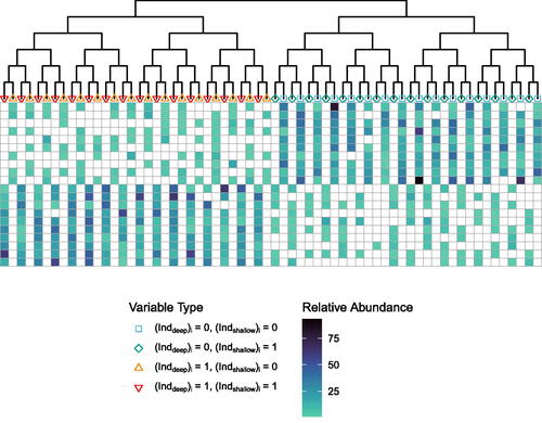
So that we can create the two different representations, we create a data matrix $\mathbf{X}\in {\mathbb{R}}^{n\times p}$ and a phylogenetic tree $\mathcal{T}$ with p leaves. These two objects are illustrated in Figure 1. The idea behind the simulation is that there are two groups of samples. There are two differences between these groups: the first is a mass difference from one half of the tree to the other, and the other an exclusion effect, in which for each pair of sister taxa, if one is present the other is absent. These two effects can be seen in Figure 1. The first group of ten samples in the top rows has a higher abundance of variables on the right-hand side of the tree (square and diamond variables) than the left-hand side of the tree (upward- and downward-pointing triangle variables), while the reverse is true for the second group of the ten samples. In addition, the first group of ten samples contains only representatives of the square and upward-pointing triangle variables, while the second group of ten samples contains only representatives of the diamond and downward-pointing triangle variables.

Fig. 1 Phylogenetic tree $\mathcal{T}$ (top) and simulated data $\mathbf{X}$ (bottom). White boxes indicate 0 abundance in the data matrix $\mathbf{X}$, and other colors from light to dark indicate low to high non-zero abundances. Samples are encoded in rows, and variables in the columns. Each variable corresponds to one tip of the tree, and the colored shapes at the tips of the tree represent the variables. The variable colors and shapes are carried through to Figure 3.

Formally, we let ${\text{Ind}}_a={({\mathbf{1}}_{n/2}^T,{\mathbf{0}}_{n/2}^T)}^T$ be the indicator of the two groups. $\mathcal{T}$ is a balanced tree with p leaves, labeled $1,\dots ,p$. Let ${\text{Ind}}_{\mathit{shallow}}\in {\{0,1\}}^p$ be such that if i and j represent sister taxa in $\mathcal{T}$, exactly one of ${({\text{Ind}}_{\mathit{shallow}})}_i,{({\text{Ind}}_{\mathit{shallow}})}_j$ is equal to 1 (indicator vector representing the exclusion effect). Call the two children of the root of $\mathcal{T}$ l and r. Let ${\text{Ind}}_{\mathit{deep}}\in {\{0,1\}}^p$ be such that ${({\text{Ind}}_{\mathit{deep}})}_i=1$ if taxon i descends from l and 0 if it descends from r (indicator vector representing the right-hand side of the tree vs. the left-hand side of the tree).

We then define(11) $$A=c_1({\text{Ind}}_a{\text{Ind}}_{shallow}^T+(1_n-{\text{Ind}}_a){(1_p-{\text{Ind}}_{shallow})}^T)\odot$$(11) (12) $$\hspace{1em}\hspace{0.17em}\text{exp}\hspace{0.17em}(c_2({\text{Ind}}_a{\text{Ind}}_{\mathit{deep}}^T+({\mathbf{1}}_n-{\text{Ind}}_a){({\mathbf{1}}_p-{\text{Ind}}_{\mathit{deep}})}^T))$$(12) (13) $$x_{ij}\sim \text{Double}\mathrm{ }\text{Pois}(a_{ij},s)$$(13) where c₁, c₂ are constants, ${\text{Ind}}_{\mathit{shallow}}$ and ${\text{Ind}}_{\mathit{deep}}$ are as defined above, $\text{exp}\hspace{0.17em}$ applied to a vector indicates the element-wise operation, and $\odot$ indicates the element-wise product.

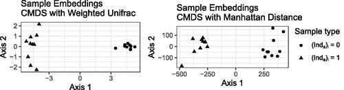
Our first step is to create CMDS embeddings of the samples in the rows of $\mathbf{X}$ using either the Manhattan distance or weighted UniFrac. The results of that embedding are shown in Figure 2, and as expected, the CMDS representation of the samples separates the samples for which ${({\text{Ind}}_a)}_i=0$ from those for which ${({\text{Ind}}_a)}_i=1$ along the first axis. Without local biplot axes, this is as far as CMDS takes us: we see that in each case, the CMDS embedding clusters the samples into the same two groups. We know in principle that weighted UniFrac uses the tree and the Manhattan distance does not, but the CMDS plot on its own provides no insight into the features of the data that go into the CMDS embeddings.

Fig. 2 Classical multidimensional scaling representation of the samples in the simulated dataset using the weighted UniFrac distance (left) and Manhattan distance (right). Each point represents a sample, and shape represents which group the sample came from.

Once we have the CMDS embeddings for weighted UniFrac and for the Manhattan distance on this dataset, we can add the local biplot axes to visualize how the variables relate to the two CMDS embedding spaces. We start with the local biplot axes for the Manhattan distance, which are shown in the bottom panel of Figure 3. The black dots are the sample points, and the colored shapes connected to line segments are the local biplot axes. The segments representing the axes are connected to the point at which the axes were computed. The biplots are as described in Section 4.3, where we plot one set of local biplot axes for each point. We see that for the Manhattan distance, the variables with positive values for the first local biplot axes are those for which ${({\text{Ind}}_{\mathit{shallow}})}_i=1$ (green diamonds and red downward triangles), and the variables with negative values for the first local biplot axes are those for which ${({\text{Ind}}_{\mathit{shallow}})}_i=0$ (blue squares and orange upward triangles). The local biplot axes are approximately the same everywhere in the space, and so we can interpret the CMDS/Manhattan distance embedding along the first axis as being approximately a projection onto a vector describing the contrast between variables with values of 0 vs. 1 for ${\text{Ind}}_{\mathit{shallow}}$ as described in Sections 5.2 and 5.4.

Fig. 3 Local biplot axes for CMDS/weighted UniFrac (top) and CMDS/Manhattan distance (bottom). One set of local biplot axes is plotted for each sample point. A segment connected to a sample point represents a local biplot axis for one variable at that sample point. The shape/color at the end of a local biplot axis represents variable type, and matches the shapes/colors of the points on the tips of the trees in Figure 1.

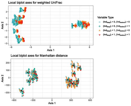
We then turn to the local biplot axes for CMDS with the weighted UniFrac distance to visualize the relationship between the variables and the CMDS embedding space for weighted UniFrac. As before, the black dots are the sample points, the colored shapes connected to line segments are the local biplot axes, the segments representing the axes are connected to the point at which the axes were computed, and the biplots are constructed as described in Section 4.3, where we plot one set of local biplot axes for each point. In contrast to the local biplot axes for CMDS with the Manhattan distance, the variables with positive values on the first local biplot axes are those for which ${({\text{Ind}}_{\mathit{deep}})}_i=1$ (orange upward and red downward triangles). The variables with negative values on the first local biplot axes are those for which ${({\text{Ind}}_{shallow})}_i=0$ (blue squares and green diamonds). The LB axes here are more variable than the LB axes for the Manhattan distance, but the signs of the first LB axes are consistent, and so we can interpret the first axis as being approximately a projection onto a vector describing the contrast between variables with value of 0 vs. 1 for ${\text{Ind}}_{\mathit{deep}}$, as described in Sections 5.2 and 5.4.

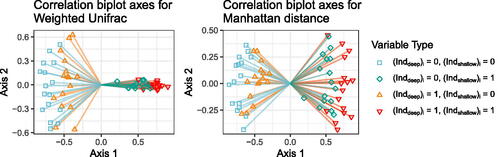
To see how much more informative the local biplot axes are from other proposals for explaining the CMDS embedding space, we create correlation biplots for CMDS with weighted UniFrac and CMDS with the Manhattan distance. The correlation biplot axes for these two embeddings are shown in the left and right panels of Figure 4, respectively. In contrast to the local biplot axes for these two embeddings, the correlation biplot axes for weighted UniFrac and the Manhattan distance are very similar to each other. In each case, the variables for which ${({\text{Ind}}_{\mathit{shallow}})}_i=0$ have positive values, while those for which ${({\text{Ind}}_{\mathit{shallow}})}_i=1$ have negative values. Although this is one explanation of the differences between the groups, it is not the only one, and in particular it is not the one that is actually used by weighted UniFrac. The reason the two sets of correlation biplot axes are so similar is that given the embeddings, the correlation biplot does not know anything about the distance used, and knows nothing about the relationship between the original data space and the embedding space. In our example, the embeddings with weighted UniFrac and the Manhattan distance were very similar, and so the correlation biplot axes were also similar.

Fig. 4 Correlation biplot axes for weighted UniFrac (left) and Manhattan distance (right). Each segment is a biplot axis. The shape/color at the end of each biplot axis represents variable type, and matches the shape/color of the points on the tips of the trees in Figure 1.

In this simulation, and generally when we have p > n, there is more than one way to separate two groups of samples. The local biplot representation in this simulation shows how two different distances implicitly use different sets of features to separate the two groups: relative abundance of the two halves of the tree (blue squares/green diamonds vs. orange and red triangles) for weighted UniFrac, and relative abundance of alternating sets of leaves on the tree (blue square/orange upward triangle vs. green diamond/red downward triangle) for the Manhattan distance. If we already knew some of the properties of weighted UniFrac and the Manhattan distance, we might have expected this result. However, the local biplot axes show us this difference very clearly and do not require us to know anything about the distances being used.

6.2 Real data for phylogenetic distances

To illustrate both how local biplot axes can help us interpret individual CMDS plots and how they can help us understand the differences between CMDS representations with different distances, we analyze data from a study of the effect of antibiotics on the gut microbiome initially described in Dethlefsen and Relman (2011). In this study, three individuals were given two courses of the antibiotic Ciprofloxacin, and stool samples were taken in the days and weeks before, during, and after each course of the antibiotic. The composition of the bacterial communities in each of these samples was analyzed using 16S rRNA sequencing (Davidson and Epperson, 2018), and the resulting dataset describes the abundances of 1651 bacterial taxa in each of 162 samples (between 52 and 56 samples were taken per individual). In addition, the taxa were mapped to a reference phylogenetic tree (Quast et al., 2013), giving us the evolutionary relationships among all the taxa in the study.

We perform CMDS and create local biplot axes for each of five different distances: the Euclidean distance, UniFrac, weighted UniFrac, the adaptive gPCA distance, and the DPCoA distance. The details of how these distances are computed are not important, as we use them only because they show dramatic and interpretable differences in the local biplot axes. All that is necessary to understand the example is that all of the distances aside from the Euclidean distance incorporate the phylogenetic information about the relationships between the bacteria in some way. The interested reader can refer to Fukuyama (2019) for more detailed discussion of the properties of these distances.

In Figure 5, we show biplots corresponding to CMDS of this dataset with each of the five distances. Each panel is a biplot, and therefore has both sample points and local biplot axes. The black shapes are the sample points, and the colored dots connected by gray line segments are the local biplot axes. The segments representing the axes are connected to the point at which the axes were computed. The color of the point at the end of a local biplot axis represents the taxonomic family that the corresponding bacteria belongs to. The biplots are as described in Section 4.3, where we plot only one set of local biplot axes to avoid cluttering the display. Axes at arbitrary points can be seen using the interactive shiny app hosted at https://jfukuyama.shinyapps.io/local-biplot-antibiotic-vis/.

Fig. 5 Biplots for CMDS of the micobiome data with each of the five distances. Samples are shown as black shapes, and biplot axes are shown as colored circles connected to gray line sigments. Local biplot axes are shown for only one point to avoid cluttering the display. Biplot axis points are colored according to the family the taxon is associated with.

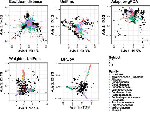
Looking first at the sample points in Figure 5, we see that the different distances give quite different representations of the samples. The Euclidean distance separates the subjects into three distinct clusters. The UniFrac and adaptive gPCA distances separate the subjects into the same three clusters but less strongly, and the weighted UniFrac and DPCoA distances do not separate the subjects at all. Upon observing this pattern, it is natural to ask what accounts for these differences. To answer that question, we can look at the local biplot axes.

The Euclidean distance, the adaptive gPCA distance, and the DPCoA distance are all generalized Euclidean distances, and since the interpretation for such distances is simpler, we will start with them. Recalling our result in Theorem 5.7 about generalized Euclidean distances and local biplot axes, we know that the location of a sample in the embedding space is a linear combination of the variables, with the weights given by the values of the local biplot axes.

For CMDS with the DPCoA distance, the local biplot axes tell us that the sample embeddings are given by a linear combination of the variables that can be approximately described as (on the first axis) a contrast between Lachnospiraceae and Ruminococcaceae/Unknown and (on the second axis) a contrast between Ruminococcaceae and Unknown.

For the adaptive gPCA distance, the local biplot axes tell us that the second axis is approximately a contrast between Ruminococcaceae and Lachnospiraceae. The first axis is more difficult to describe in terms of the family the bacterial taxa belong to. Although it is not evident from the plot itself, the local biplot axes tend to fall into small clusters, and these clusters tend to be groups of closely related bacterial taxa. This phenomenon can be seen on the shiny app, at https://jfukuyama.shinyapps.io/local-biplot-antibiotic-vis/. Accordingly, just as the first axis in CMDS with the DPCoA distance can be described as approximately a linear combination of variables corresponding to bacterial families, the first axis in CMDS with the adaptive gPCA distance can be described as approximately a linear combination of variables corresponding to smaller groups of related bacteria.

For CMDS with the Euclidean distance, we can again describe the positions of the samples as a linear combination of the variables, with weights given by the local biplot axes. In this case, however, there is no relationship between taxonomic family and the location of the biplot axes, and so a simple explanation of the embedding space is not available.

We turn next to the biplots for weighted UniFrac and unweighted UniFrac. Neither is a generalized Euclidean distance, and so the local biplot axes are not constant for either biplot. However, we do see that the local biplot axes shown for weighted UniFrac are approximately the same as those for DPCoA reflected over the vertical axis. If we looked at the local biplot axes for other points in the space, we would see that they are also approximately constant across the space. This suggests that the sample embeddings given in the weighted UniFrac representation have a similar interpretation as those in the DPCoA representation: the first axis is given by a contrast between Lachnospiraceae and Ruminococcaceae, and the second axis is a contrast between Lachnospiraceae/Ruminococcaceae and Unknown.

Finally, looking at the local biplot axes for CMDS with unweighted UniFrac, we see (in the interactive version of the plot) that the local biplot axes are qualitatively similar to those for CMDS with the adaptive gPCA distance. That is, there is some clustering of the local biplot axes, and the clusters tend to correspond to groups of closely related bacteria. This suggests to us that the embedding space for CMDS with unweighted UniFrac can be described in a similar way as the embedding space for CMDS with the adaptive gPCA distance: moving from one part of the embedding space to another corresponds to changing abundances in small groups of closely-related bacteria.

Overall, we find that the local biplot axes help us interpret the CMDS embedding space. The local biplot axes give us insight into the particular CMDS representation at hand: which sets of bacterial taxa are likely to be over- or under-represented in particular samples or particular regions of the embedding space. This is information that is not traditionally available in CMDS but is of great importance to the consumers of such diagrams. In this particular instance, even if we came in knowing nothing about the phylogenetic distances, the local biplot axes give us some insight into their properties. Specifically, we see that the local biplot axes show variable amounts of clustering by taxonomic group. If we make the analogy to PCA biplot axes, this tells us that CMDS with the phylogenetic distances are similar to a PCA in which we encourage the principal axes to have similar values for similar taxa. The strength of this “encouragement” is the largest for the DPCoA and weighted UniFrac distances, intermediate for the unweighted UniFrac and adaptive gPCA distances, and non-existent for the Euclidean distance. This result is in line with previous work (Fukuyama, 2019) showing empiricially such a gradient in a larger set of phylogenetically-informed distances.

7 Discussion

We have introduced local biplot axes as a new tool for gaining insight into the normally opaque technique of classical multidimensional scaling. We showed that these local biplot axes are a natural extension of PCA biplot axes and that there is a close connection between these axes and generalized principal components. Our extension of the result on the equivalence principal components and CMDS with the Euclidean distance to gPCA and CMDS with a generalized Euclidean distance gives us greater insight into the relationship between data space and embedding space for CMDS. It particular, it suggests that for an arbitrary distance, if the local biplot axes are approximately constant, the distance can be well approximated by a generalized Euclidean distance and that the generalized Euclidean distance providing the approximation is a function of the local biplot axes. Because generalized Euclidean distances can be understood as the standard Euclidean distance on a linear transformation of the input variables, this result helps us interpret what variables or features in the data are important. This idea is related to a recent biplot proposal that uses “weighted Euclidean distances”, that is, the subset of generalized Euclidean distances $d_{\mathbf{A}}$ with $\mathbf{A}$ diagonal instead of positive definite (Greenacre and Groenen, 2016).

Even in the case where the local biplot axes are far from being constant on the input variable space, the local biplot axes allow us to investigate whether there are regions of local linearity (regions in which the local biplot axes are constant or approximately constant), and therefore where we might be able to approximate the distance as a generalized Euclidean distance or approximate the CMDS map as a linear map from data space to embedding space. This gives us much more insight into the relationship between data and embedding space than is available either with CMDS on its own (no information) or other proposals for biplots for CMDS, which tend to be about a global linear approximation (Satten et al., 2017; Wang et al., 2019; Greenacre, 2017; Greenacre and Groenen, 2016).

The information the local biplot axes provide about the relationship between the variables and the CMDS embedding space is particularly important if the distance being used for CMDS was designed to incorporate the analyst’s intuition about important features of the data for the particular area of application. We showed this using some non-standard phylogenetically-informed distances from the microbiome field. The intuition encoded in these distances is that the tree provides important information, and an explanation of the difference between the groups as over- or under-representation of large groups of related taxa is more useful than an explanation in terms of groups of unrelated taxa. The local biplot axes clearly show that CMDS with these distances is using the tree in this way.

Our simulated data example showed that local biplots can uncover substantive differences in the relationship between data space and embedding space, even in cases where CMDS with two different distances gives the same embedding of the samples. Our real data example showed that local biplots can suggest scientifically relevant reasons for the differences in the representations of the samples provided by CMDS with different distances. They can also suggest more general properties of the distances used: in this case, we saw that different phylogenetic distances appear to implicitly smooth the variables along the phylogenetic tree to different degrees.

There are several avenues for future work. The same basic idea that we use here could be applied to other forms of MDS. So long as it is possible to add a supplemental point to an MDS diagram and compute sensitivities, it is possible to create the same kinds of local biplots we define here. In addition to making the resulting visualizations more useful, creating local biplots for other kinds of MDS would give us insight into how the other methods work. Additionally, since our results suggest that approximately constant local biplot axes should imply that the distances are approximately of the form of a generalized Euclidean distance, another potential line of inquiry is to quantify the approximation or investigate how to choose the best generalized Euclidean distance for the approximation. Similarly, to identify regions of local linearity, we would need a way to quantify the similarity of the local biplot axes in different regions of the space, and it is not immediately obvious what the best measure would be for this task. Other potential areas for investigation include developing the relationship between distances and probabilistic models through the relationship between generalized Euclidean distances and the probabilistic interpretation of generalized PCA, or using the LB axes as a starting point for confidence ellipses for CMDS.

Supplemental Materials

Appendix:

A pdf containing supplemental proofs and discussion. (pdf)

R package for local biplots:

An R package containing code to create the local biplots described in the paper is available at https://github.com/jfukuyama/localBiplots. The package contains, as a vignette, the code used to create the simulated data and the associated plots, the antibiotic data used in the analysis, and the code used to create the figures corresponding to the antibiotic data.

References

- Allen, G. I., Grosenick, L. and Taylor, J. (2014), ‘A generalized least-square matrix decomposition’, Journal of the American Statistical Association 109(505), 145–159. DOI: 10.1080/01621459.2013.852978.
- Daunis-i Estadella, J., Thió-Henestrosa, S. and Mateu-Figueras, G. (2011), ‘Including supplementary elements in a compositional biplot’, Computers & Geosciences 37(5), 696–701.
- Davidson, R. M. and Epperson, L. E. (2018), Microbiome sequencing methods for studying human diseases, in ‘Disease Gene Identification’, Springer, pp. 77–90.
- Dethlefsen, L. and Relman, D. A. (2011), ‘Incomplete recovery and individualized responses of the human distal gut microbiota to repeated antibiotic perturbation’, Proceedings of the National Academy of Sciences 108(Supplement 1), 4554–4561. DOI: 10.1073/pnas.1000087107.
- Fukuyama, J. (2019), ‘Emphasis on the deep or shallow parts of the tree provides a new characterization of phylogenetic distances’, Genome Biology 20(1), 131. DOI: 10.1186/s13059-019-1735-y.
- Gabriel, K. R. (1971), ‘The biplot graphic display of matrices with application to principal component analysis’, Biometrika 58(3), 453–467. DOI: 10.1093/biomet/58.3.453.
- Gabriel, K. R. (2002), ‘Goodness of fit of biplots and correspondence analysis’, Biometrika 89(2), 423–436. DOI: 10.1093/biomet/89.2.423.
- Gower, J. C. (1966), ‘Some distance properties of latent root and vector methods used in multivariate analysis’, Biometrika 53(3-4), 325–338. DOI: 10.1093/biomet/53.3-4.325.
- Gower, J. C. (1968), ‘Adding a point to vector diagrams in multivariate analysis’, Biometrika 55(3), 582–585. DOI: 10.1093/biomet/55.3.582.
- Gower, J. C. and Harding, S. A. (1988), ‘Nonlinear biplots’, Biometrika 75(3), 445–455. DOI: 10.1093/biomet/75.3.445.
- Gower, J., Groenen, P. and van de Velden, M. (2010), ‘Area biplots’, Journal of Computational and Graphical Statistics 19(1), 46–61. DOI: 10.1198/jcgs.2010.07134.
- Greenacre, M. (2013), ‘Contribution biplots’, Journal of Computational and Graphical Statistics 22(1), 107–122. DOI: 10.1080/10618600.2012.702494.
- Greenacre, M. (2017), ‘Ordination with any dissimilarity measure: A weighted Euclidean solution’, Ecology 98(9), 2293–2300. DOI: 10.1002/ecy.1937.
- Greenacre, M. J. (1984), ‘Theory and applications of correspondence analysis’.
- Greenacre, M. J. (2010), Biplots in practice, Fundacion BBVA.
- Greenacre, M. J. and Groenen, P. J. (2016), ‘Weighted euclidean biplots’, Journal of Classification 33(3), 442–459. DOI: 10.1007/s00357-016-9213-7.
- Holmes, S. (2008), Multivariate data analysis: The French way, in ‘Probability and Statistics: Essays in Honor of David A. Freedman’, Institute of Mathematical Statistics, pp. 219–233.
- Lozupone, C. A., Hamady, M., Kelley, S. T. and Knight, R. (2007), ‘Quantitative and qualitative β diversity measures lead to different insights into factors that structure microbial communities’, Applied and Environmental Microbiology 73(5), 1576–1585. DOI: 10.1128/AEM.01996-06.
- Mahalanobis, P. C. (1936), ‘On the generalized distance in statistics’, Proceedings of the National Institute of Sciences of India 2(1), 49–55.
- McCune, B., Grace, J. B. and Urban, D. L. (2002), Analysis of Ecological Communities, Vol. 28, MjM Software Design, Gleneden Beach, OR.
- Quast, C., Pruesse, E., Yilmaz, P., Gerken, J., Schweer, T., Yarza, P., Peplies, J. and Glöckner, F. O. (2013), ‘The SILVA ribosomal RNA gene database project: Improved data processing and web-based tools’, Nucleic Acids Research 41(D1), D590–D596. DOI: 10.1093/nar/gks1219.
- Satten, G. A., Tyx, R. E., Rivera, A. J. and Stanfill, S. (2017), ‘Restoring the duality between principal components of a distance matrix and linear combinations of predictors, with application to studies of the microbiome’, PLoS One 12(1), e0168131. DOI: 10.1371/journal.pone.0168131.
- Torgerson, W. S. (1958), Theory and Methods of Scaling, Vol. 460, Wiley, Oxford, England.
- Wang, Y., Randolph, T. W., Shojaie, A. and Ma, J. (2019), ‘The generalized matrix decomposition biplot and its application to microbiome data’, mSystems 4(6). URL: https://msystems.asm.org/content/4/6/e00504-19