Inference and Computation for Sparsely Sampled Random Surfaces

Abstract

Nonparametric inference for functional data over two-dimensional domains entails additional computational and statistical challenges, compared to the one-dimensional case. Separability of the covariance is commonly assumed to address these issues in the densely observed regime. Instead, we consider the sparse regime, where the latent surfaces are observed only at few irregular locations with additive measurement error, and propose an estimator of covariance based on local linear smoothers. Consequently, the assumption of separability reduces the intrinsically four-dimensional smoothing problem into several two-dimensional smoothers and allows the proposed estimator to retain the classical minimax-optimal convergence rate for two-dimensional smoothers. Even when separability fails to hold, imposing it can be still advantageous as a form of regularization. A simulation study reveals a favorable bias-variance tradeoff and massive speed-ups achieved by our approach. Finally, the proposed methodology is used for qualitative analysis of implied volatility surfaces corresponding to call options, and for prediction of the latent surfaces based on information from the entire dataset, allowing for uncertainty quantification. Our cross-validated out-of-sample quantitative results show that the proposed methodology outperforms the common approach of pre-smoothing every implied volatility surface separately. Supplementary materials for this article are available online.

Keywords:

• Functional data
• Implied volatility
• Kernel smoothing
• Prediction
• Separability

1 Introduction

The term random surfaces refers to continuous data on a two-dimensional domain. Such datasets consist of multiple independent replications of some underlying process $X=(X(t,s),t\in \mathcal{T},s\in \mathcal{S})$, forming a random sample $X_1,\dots ,X_N$, and can be tackled in the context of functional data analysis (FDA), see Ramsay and Silverman (2005, 2007). In practice, surface-valued data cannot be observed as infinite-dimensional objects, one instead observes only a finite number of measurements per surface. The classical split in literature (see Zhang and Wang 2016, for a comprehensive overview) consists of two measurement regimes: the dense sampling and the sparse sampling. The former considers the setting where the surface data are recorder densely enough (usually on a grid) so they can be worked with as if they were truly infinite dimensional, possibly after a pre-smoothing step, while retaining the same asymptotic properties as truly infinite dimensional data (Hall, Müller, and Wang 2006). The sparse regime, however, requires a different approach. Here, the surfaces are observed only on a small (varying) number of irregular locations, which also vary across the surfaces and are corrupted with measurement errors. If such observations are gridded, which is common for computational reasons, the resulting matrix-valued samples contain many missing entries. Densely observed random surfaces arise frequently in medical imaging, linguistics (Pigoli et al. 2018), or climate studies (Gneiting, Genton, and Guttorp 2006). Examples of sparsely observed random surfaces include longitudinal studies, where only a part of a functional profile is measured at each visit (Lopez et al. 2020), geolocalized data (Yarger, Stoev, and Hsing 2020; Zhang and Li 2020; Wang, Wong, and Zhang 2020), or financial data (Fengler 2009; Kearney, Cummins, and Murphy 2018).

Regardless of the sampling regime, any functional data analysis will begin by estimating two fundamental objects: the mean function $\mu (t,s)=\mathbb{E}X(t,s)$ and the covariance kernel $c(t,s,t\prime ,s\prime )=\text{cov}(X(t,s),X(t\prime ,s\prime ))$. These ought to be estimated nonparametrically, since availability of replicated observations should allow so. While the mean has the same dimension as the underlying process itself, the covariance is an object of a higher dimension, and its estimation thus suffers from the curse of dimensionality. The size of a general covariance often poses both computational and statistical issues, for example, restricting the resolution of the grid one can handle (Aston, Pigoli, and Tavakoli 2017; Masak, Sarkar, and Panaretos 2020).

Separability of the covariance is a popular nonparametric assumption to reduce the statistical and computational burden, which arises when working on a multi-dimensional domain. Well-known and often coupled together with parametric models in the field of spatial statistics (see e.g., De Iaco, Myers, and Posa 2002, and references therein), separability has lately attracted a lot of attention also from the nonparametric viewpoint of FDA (Bagchi and Dette 2020; Constantinou, Kokoszka, and Reimherr 2017; Masak and Panaretos 2019; Dette, Dierickx, and Kutta 2020). Intuitively, it allows one to decouple the dimensions, regarding the random surfaces as an enlarged ensemble of random curves instead. Specifically, separability assumes that the full covariance can be written as a product of covariance kernels corresponding to individual dimensions, that is:$$c(t,s,t\prime ,s\prime )=a(t,t\prime )b(s,s\prime )$$for some bivariate kernels $a=a(t,t\prime )$ and $b=b(s,s\prime )$. Thus separability decomposes the four-dimensional covariance kernel into two kernels, each of the same dimensionality as the mean function.

Though separability cannot always be justified in the context of applied problems (Rougier 2017), it is nevertheless frequently imposed because of the computational advantages it entails (Gneiting, Genton, and Guttorp 2006; Genton 2007; Pigoli et al. 2018). And, while wrongfully assuming separability introduces a bias, it may still lead to improved estimation and prediction due to an implicit bias-variance tradeoff. What is certain is that separability greatly reduces computational costs of both the estimation and prediction tasks.

To the best of our knowledge, the aforementioned properties of separability have been mostly explored in the case of densely observed data. In the sparse regime, there is no procedure for the nonparametric estimation of a separable covariance. Methodology designed for the densely observed surfaces does not apply, and methods designed for sparsely observed curves cannot feasibly be extended to surfaces, as we will later argue. Since sparse data are generally associated with higher computational complexity (extra costs associated with smoothing) as well as higher statistical complexity (variance is inflated due to sparse measurements burdened by noise), it appears that the gains stemming from separability could be even larger in the sparse regime.

The goal of this article is to leverage the separability assumption to reduce complexity of covariance estimation down to that of mean estimation when working under the sparse regime. The method of choice for sparsely observed functional data on one-dimensional domains is the PACE approach (Yao, Müller, and Wang 2005), which is based on kernel regression smoothers. A naive generalization of PACE to a two-dimensional domain would entail a computationally infeasible local linear smoothing step in a four-dimensional space. Instead, we demonstrate how to make careful use of separability to collapse the four-dimensional smoother into several two-dimensional surface smoothers. Consequently, the estimation of the mean, the covariance, and the noise level all become of similar computational complexity. While this complexity depends on a specific smoothing algorithm, our methodology can benefit from any speed-ups (such as those proposed by Chen and Jiang 2017) just as well as the naive generalization of PACE. Reducing the dimensionality of the problem always cuts down computations, regardless of the specific smoothing algorithm used (see Appendix I.2, supplementary materials).

Second, our asymptotic theory shows that the estimators match the minimax optimal convergence rates for two-dimensional smoothing problems. Moreover, our simulation study demonstrates the enormous computational gains offered by separability, the statistical gains when the ground-truth is separable, and a favorable bias-variance tradeoff when the truth is in fact not separable.

Finally, we illustrate the benefits of our approach on a qualitative analysis as well as prediction of implied volatility surfaces corresponding to call options. Here, one surface corresponds to a fixed asset (e.g., a stock), for which the right to buy it for an agreed-upon strike price (first dimension) at a future time to expiration (second dimension) is traded. The value of implied volatility at given strike and time to expiration is derived directly from observed market data (the option prices), by the well-known and commonly used Black-Scholes formula (Black and Scholes 1973; Merton 1973). The implied volatilities are preferred over the option prices, since they are dimensionless quantities, allow for a direct comparison of different assets, and are well familiar to practitioners. Since the options are traded only for a finite number of strikes and times to expiration, which vary across different surfaces, the observed data consist of a sparse ensemble. The interpolation of such an ensemble is a typical objective in financial mathematics as the latent implied volatility surfaces are of interest for other tasks such as prediction (forecasting) of option prices (Hull 2006). The common practice is to interpolate or smooth the measurements for every surface independently. For example, Cont and Da Fonseca (2002) used pre-smoothing by local polynomial regression, evaluating an individual smoother for every single surface. This approach may, however, pose issues when the available sparse measurements for a given surface are concentrated only on a subset of the domain, which is often the case. Once the predicted surfaces are fed into a subsequent predictive models, the naively extrapolated parts of the surface are given the same weight as the more reliable interpolated parts. Instead, we advocate for the idea of “borrowing strength” for the purpose of predicting the latent surfaces via best linear unbiased prediction using the information from the entire dataset, which also allows for uncertainty quantification (Yao, Müller, and Wang 2005). Under separability, we only need to use two-dimensional surface smoothing, which is the case of the pre-smoothing approach as well. At the same time, the proposed methodology outperforms the pre-smoothing approach in terms of prediction error.

2 Methodology

2.1 Model and Observation Scheme

We assume the existence of iid latent surfaces $X_n\in {\mathcal{L}}^2({[0,1]}^2),n=1,\dots ,N$, which are mean-square continuous with continuous sample paths. We denote the mean function as $\mu =\mu (t,s)$, where$$\mu (t,s)=\mathbb{E}{X}_1(t,s),\mathrm{\hspace{1em}}\mathrm{\hspace{1em}}t,s\in [0,1],$$and the covariance kernel as $c=c(t,s,t\prime ,s\prime )$, where$$\begin{array}{c}c(t,s,t\prime ,s\prime )=\mathbb{E}\left[\left(X_1(t,s)-\mu (t,s)\right)\left(X_1(t\prime ,s\prime )-\mu (t\prime ,s\prime )\right)\right],\\ t,s,t\prime ,s\prime \in [0,1].\end{array}$$

We think of the first dimension as being temporal, denoted by variable t, and the second dimension as being spatial, denoted by variable s, though this convention is only made for the purposes of presentation.

The crucial assumption in this paper is that of separability of the covariance:

1. The covariance kernel of the random surfaces $X_1,\dots ,X_N$ satisfies(1) $$c(t,s,t\prime ,s\prime )=a(t,t\prime )b(s,s\prime ),\mathrm{\hspace{1em}}\mathrm{\hspace{1em}}t,s,t\prime ,s\prime \in [0,1],$$(1)

for a purely temporal covariance $a=a(t,t\prime )$ and some purely spatial covariance $b=b(s,s\prime )$.

The process $X\in {\mathcal{L}}^2({[0,1]}^2)$ is separable if it is, for example, an outer product of two independent univariate processes (a purely temporal one and a purely spatial one). In that case, apart from the covariance, the mean function also separates into a product of a purely temporal and a purely spatial functions. However, a process can have a separable covariance even when it is not itself separable (Rougier 2017), for example, the mean function may not be separable. We do not assume separability of the latent process itself, we only assume separability of its covariance in the sense of (1).

We work under the sparse sampling regime, where every surface is observed only at a finite number of irregularly distributed locations, and those measurements are corrupted by independent additive errors. For the n-th latent surface X_n , the number of measurements M_n as well as the locations of the measurements $\{(t_{nm},s_{nm})|m=1,\dots ,M_n\}\subset {[0,1]}^2$ are considered random, and the observations are given by the errors-in-measurements model (Yao, Müller, and Wang 2005; Li and Hsing 2010; Zhang and Wang 2016):(2) $$Y_{nm}=X_n(t_{nm},s_{nm})+{\epsilon }_{nm},\hspace{1em}m=1,\dots ,M_n,n=1,\dots ,N,$$(2) where ${\epsilon }_{nm}$ are iid with $\mathbb{E} {\epsilon }_{nm}=0$ and $\text{var}({\epsilon }_{nm})={\sigma }^2>0$ being the noise level.

2.2 Motivation

In this section, we assume for simplicity that the mean is zero, and provide a heuristic description of how one might estimate the separable covariance (1). Note that we have$$\begin{array}{c}\text{cov}(Y_{nm},Y_{nm\prime })=a(t_{nm},t_{nm\prime })b(s_{nm},s_{nm\prime })+{\sigma }^2{1}_{[m=m\prime ]},\\ n=1,\dots ,N,m,m\prime =1,\dots ,M_n.\end{array}$$

Consider the “raw covariances” $G_{\mathit{nmm}\prime }:=Y_{nm}{Y}_{nm\prime }$. Ignoring the assumption of separability, one could attempt to “lift” the PACE approach (Yao, Müller, and Wang 2005) up to higher dimensions. This amounts to plotting the raw covariances as a scatterplot in a four-dimensional domain, discarding the diagonal covariances burdened by noise, and using a surface smoother to obtain an estimator of the covariance. We refer to this procedure as 4D smoothing, see Appendix I.2, supplementary materials for details. However, there are two issues with 4D smoothing. The curse of dimensionality results in an estimator of poor quality, unless surfaces are observed relatively densely and many replications are available. And, especially when the latter is true, the computational costs of smoothing in a higher dimension can be excessive. We make the assumption of separability mainly to cope with these two issues, which is often the case in the literature already when working with fully observed data (Gneiting, Genton, and Guttorp 2006; Pigoli et al. 2018). We do not see separability as a critical modeling assumption, but rather as a regularization, which possibly introduces a bias. Separability reduces both the statistical and the computational complexity of the covariance estimation task. This is always important when working with random surfaces, whatever their mode of observation, but becomes particularly crucial when working with sparsely observed surfaces.

In the following, we provide a heuristic on how separability can be used to our advantage in the sparse observation regime. Assuming zero mean for now, we have$$\mathbb{E}{G}_{\mathit{nmm}\prime }=\mathbb{E}{Y}_{nm}{Y}_{nm\prime }=a(t_{nm},t_{nm\prime })b(s_{nm},s_{nm\prime })+{\sigma }^2\mathrm{ }{1}_{[m=m\prime ]}.$$

Imagine for a moment that the spatial kernel $b=b(s,s\prime )$ is known, and consider the set of values(3) $$\left\{\frac{Y_{nm}{Y}_{nm\prime }}{b(s_{nm},s_{nm\prime })}|m,m\prime =1,\dots ,M_n,m\ne m\prime ,n=1,\dots ,N\right\}.$$(3)

The expectation of every point in this set is $a(t_{nm},t_{nm\prime })$, so we can chart these points in a scatterplot as$$\left(t_{nm},t_{nm\prime },\frac{Y_{nm}{Y}_{nm\prime }}{b(s_{nm},s_{nm\prime })}\right),$$and use a two-dimensional surface smoother to obtain an estimator of $a=a(t,t\prime )$.

Correspondingly, if one knew the temporal kernel $a=a(t,t\prime )$ instead, the set of values (3) (with a in the denominator instead of b) could be arranged against s_nm and $s_{nm\prime }$ to obtain an estimator of $b=b(s,s\prime )$. When neither the temporal kernel a nor the spatial b is known, one can start with a fixed b and iterate between updates of a and b, smoothing a scatterplot once per every single update.

However, there are two issues with such an approach. First, for small denominators, the corresponding points on the scatterplot are not reliable, and using them as they are can have a severe negative impact on estimation quality. Second, unless very few observations per surface are available, the procedure above is computationally very demanding, see Appendix I.5, supplementary materials.

To cope with these issues, we use weights for the surface smoother and use gridding, that is, split the domain into disjoint intervals and work on a grid. While gridding can significantly reduce computations already on a univariate domain (Yao, Müller, and Wang 2005), the gains are much bigger in higher dimensions. In the following section, we introduce our methodology in full from the theoretical perspective, while computational aspects are deferred to Appendix I.2, supplementary materials.

2.3 Estimation of the Model Components

We use local linear regression surface smoothers (Fan and Gijbels 1996) to formalize the heuristic described in the previous section and estimate the components of the model from Section 2.1, that is, the mean $\mu =\mu (t,s)$, the temporal kernel $a=a(t,t\prime )$, the spatial kernel $b=b(s,s\prime )$, and the noise level ${\sigma }^2$.

By applying a surface smoother to the set $\{(x_k,y_k,z_k)|k=1,\dots ,M\}\subset {\mathbb{R}}^3$ with given weights $\left\{w_k\right|k=1,\dots ,M\}$, we understand calculating ${\widehat{\gamma }}_0={\widehat{\gamma }}_0(x,y)$ as the minimizer of the weighted sum of squares$$\begin{array}{c}(\widehat{{\gamma }_0},\widehat{{\gamma }_1},\widehat{{\gamma }_2})=\text{arg} {\text{min}}_{{\gamma }_0,{\gamma }_1,{\gamma }_2}\sum _{k=1}^{M}K\left(\frac{x-x_k}{h_1}\right)K\left(\frac{y-y_k}{h_2}\right)w_k\\ \hspace{1em}{[z_k-{\gamma }_0-{\gamma }_1(x-x_k)-{\gamma }_2(y-y_k)]}^2\end{array}$$for every fixed $(x,y)\in {[0,1]}^2$, where $K(·)$ is a smoothing kernel function and $h_1,h_2>0$ are bandwidths. Throughout the paper, we use the Epanechnikov kernel, use cross-validation to select the bandwidths, and mention weights only when they are not all equal.

First, we estimate the mean by applying the surface smoother to the set(4) $$\{(t_{nm},s_{nm},Y_{nm})|m=1,\dots ,M_n,n=1,\dots ,N\}.$$(4)

Denote the resulting estimator by $\widehat{\mu }=\widehat{\mu }(t,s)$.

Next, consider the “raw” covariances $G_{\mathit{nmm}\prime }=[Y_{nm}-\widehat{\mu }(t_{nm},s_{nm})][Y_{nm\prime }-\widehat{\mu }(t_{nm\prime },s_{nm\prime })].$ We begin by applying the surface smoother to the set$$\{(t_{nm},t_{nm},G_{\mathit{nmm}\prime })|m,m\prime =1,\dots ,M_n, m\ne m\prime ,n=1\dots ,N\}$$to obtain a preliminary estimator of $a=a(t,t\prime )$, denoted by ${\widehat{a}}_0={\widehat{a}}_0(t,t\prime )$. Then we use this preliminary estimator to calculate a proxy of $b=b(s,s\prime )$, like we described in the previous section. Namely, we apply the surface smoother to the set(5) $$\begin{array}{c}\{\left(s_{nm},s_{nm\prime },\frac{G_{\mathit{nmm}\prime }}{{\widehat{a}}_0(t_{nm},t_{nm\prime })}\right)|m,m\prime =1,\dots ,M_n,\\ m\ne m\prime ,n=1\dots ,N\}\end{array}$$(5) using weights $\{{\widehat{a}}_0^2(t_{nm},t_{nm\prime })\}$ to obtain ${\widehat{b}}_0={\widehat{b}}_0(s,s\prime )$. If the denominator in the set above is ever zero, we remove the corresponding point from the set. Note that since the weights are equal exactly to the denominators squared, it makes sense even formally that such a point is never considered for the surface smoother. As the next step, we refine our estimator of a by applying the surface smoother to the set(6) $$\begin{array}{c}\{\left(t_{nm},t_{nm\prime },\frac{G_{\mathit{nmm}\prime }}{{\widehat{b}}_0(s_{nm},s_{nm\prime })}\right)|m,m\prime =1,\dots ,M_n,\\ m\ne m\prime ,n=1\dots ,N\}\end{array}$$(6) using weights $\{{\widehat{b}}_0^2(s_{nm},s_{nm\prime })\}$ from which we obtain $\widehat{a}=\widehat{a}(t,t\prime )$. Finally, we refine the estimator of b by applying the surface smoother to set (5) with ${\widehat{a}}_0$ replaced by $\widehat{a}$, resulting in the estimator $\widehat{b}=\widehat{b}(s,s\prime )$.

Finally, once both the mean and the separable covariance have been estimated, it remains to estimate the noise level ${\sigma }^2$, which is of interest for example, for the purposes of prediction. We apply the surface smoother to the set $\left\{(t_{nm},s_{nm},G_{\mathit{nmm}})|m=1,\dots ,M_n,n=1\dots ,N\right\}$ to obtain $\widehat{V}=\widehat{V}(t,s)$. Note that since $\mathbb{E}{G}_{\mathit{nmm}}\approx a(t_{nm},t_{nm})b(s_{nm},s_{nm})+{\sigma }^2$, we can estimate ${\sigma }^2$ by$${\widehat{\sigma }}^2=4{\int }_{1/4}^{3/4}{\int }_{1/4}^{3/4}[\widehat{V}(t,s)-\widehat{a}(t,t)\widehat{b}(s,s)]\mathit{dtds},$$where (similarly to Yao, Müller, and Wang 2005) we integrate only along the middle part of the domain to mitigate boundary issues.

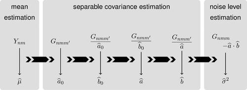
The workflow of the estimation scheme described above is visualized in Figure 1. The main novelty of our approach lies in the part where the separable covariance is estimated. Separability allows us to reduce dimensionality of the problem. Hence only two-dimensional smoothing is required, while a straightforward multi-dimensional generalization of for example, the PACE approach (Yao, Müller, and Wang 2005) not using separability would require four-dimensional smoothing to estimate the covariance.

Fig. 1 Workflow of the proposed estimation procedure. We estimate firstly the mean from the data $\left\{Y_{nm}\right\}$, then the separable covariance (in several steps) from the raw covariances $\left\{G_{\mathit{nmm}\prime }\right\}$, and finally the noise level. A surface smoother over a 2D domain is used in every step (once per a single thin arrow).

The estimation of the separable terms can be viewed as an iterative procedure, where either a or b is kept fixed while the other term is being updated. The initializing estimate ${\widehat{a}}_0$ is also obtained in this way, starting from ${\widehat{b}}_0\equiv 1$. A natural question is whether one should iterate this process until convergence, or simply stop after a single step, and use for example, ${\widehat{a}}_0$ as the estimator of a. The approach we advocate for uses exactly two steps (for both a and b). The reason is the following. As will be shown in Section 3, the asymptotic distribution of $\widehat{b}$ does not depend on ${\widehat{a}}_0$, and similarly for $\widehat{a}$. This fact follows from separability. However, given the motivation in the previous section, one can anticipate the finite sample performance of $\widehat{a}$ to be better than that of ${\widehat{a}}_0$, which is verified in our simulation study. Also, one can think of the first step as estimating the optimal weights consistently, and the second step as using those consistently estimated weights to produce the estimators. Naturally, one can use more than two steps, and the optimal number of steps can be chosen in a data-driven way using cross-validation, cf Appendix I.3, supplementary materials. Still, we recommend using exactly two steps due to the conceptual simplicity.

One of the distinctive features of our methodology is the use of this explicit weighing scheme, where the weights for each of the two covariance kernels depend on the other covariance kernel. We explain why this is done in the following example. A more precise justification for the specific (quadratic) form of the weights, which requires some additional background, is deferred to Appendix I.1, supplementary materials.

Example 1.

Assume X₁ is observed at four locations only, as depicted in Figure 2. First, let us describe the 4D smoothing estimator at a fixed location $(t,s,t\prime ,s\prime )$: X₁ contributes to $\widehat{c}(t,s,t\prime ,s\prime )$ only if there is a pair of two locations, where X₁ is observed, such that one of the locations is close to (t, s), and the other is close to $(t\prime ,s\prime )$. In this case, closeness in time, resp. space, is measured by the bandwidths h_t , resp. h_s . In Figure 2 (left), only a single pair of locations contributes to estimation at $(t,s,t\prime ,s\prime )$.

Fig. 2 A single random surface is observed at four locations (depicted by “$x$”), and these observations contribute differently to estimation of the covariance at a fixed location $(t,s,t\prime ,s\prime )$ in the case of 4D smoothing (left) and one step of the proposed approach leading to the estimator of $a(t,t\prime )$ (right). The gray areas depict active neighborhoods and the dashed lines depict the contributing raw covariances (products of the values at the connected locations).

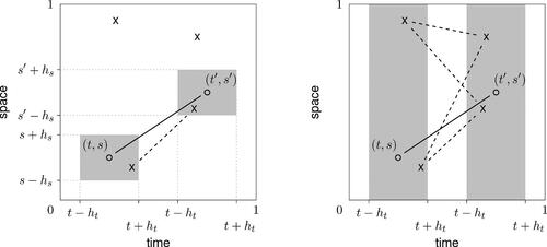
Second, let us contrast this to a single step in the proposed estimating procedure. Assume that $b=b(s,s\prime )$ is fixed in the current step, and we are estimating $a=a(t,t\prime )$. In this step, the spatial dimensions are not explicitly considered, smoothing is conducted only in the temporal dimensions. Hence the product of any two locations, where X₁ is observed, contributes to $\widehat{a}$, as long as the locations are close to (t, s) and $(t\prime ,s\prime )$ in the temporal domain. In the situation displayed in Figure 2 (right), this leads to four contributing raw covariances. In other words, when estimating the temporal part of the covariance at $(t,s,t\prime ,s\prime )$, we can consider even raw covariances, which are spatially far from $(t,s,t\prime ,s\prime )$. This is meaningful due to separability. The adopted weighting scheme then ensures that raw covariances arising from points which are spatially distant are appropriately weighted.

To sum up, 4D smoothing can be understood as local averaging over information about $c(t,s,t\prime ,s\prime )$ captured in raw covariances. Under separability, however, the proposed methodology borrows information in a different manner, always allowing for more freedom in one dimension or the other, depending on which dimension is currently held fixed.

2.4 Marginalization on a Grid

By marginalization, we mean preparation of the raw covariances for 2D smoothing step, that is, charting the raw covariances either in time or in space and weighting them as in formulas (6) and (5). In this section, we will show that scatter points can be pooled together during the marginalization process to save computations during the subsequent smoothing step, when the data are observed (or rounded to) a common grid. The associated computational advantages are discussed in Appendix I.2.

Assume for the remainder of this section that data from the measurement scheme (2) arrive as matrices ${\mathbf{Y}}_1,\dots ,{\mathbf{Y}}_N\in {\mathbb{R}}^{d_1\times d_2}$ with only some of their entries known, that is, most of the entries are missing. The marginal covariance kernels $a=a(t,t\prime )$ and $b=b(s,s\prime )$ are replaced by matrices $\mathbf{A}\in {\mathbb{R}}^{d_1\times d_1}$ and $\mathbf{B}\in {\mathbb{R}}^{d_2\times d_2}$, respectively. We assume again for simplicity that the mean $\mu =\mu (t,s)$ is zero. The raw covariances then form a tensor ${\mathbf{G}}_n={\mathbf{Y}}_n\otimes {\mathbf{Y}}_n\in {\mathbb{R}}^{d_1\times d_2\times d_1\times d_2}$ with entries ${\mathbf{G}}_n[i,j,i\prime ,j\prime ]={\mathbf{Y}}_n[i,j]{\mathbf{Y}}_n[i\prime ,j\prime ]$.

Again, like before, assume that $\mathbf{B}$ is fixed for now, and we are using the surface smoother on the discrete equivalent to set (6), that is(7) $$\begin{array}{c}\left\{\left(i,i\prime ,\frac{{\mathbf{G}}_n[i,j,i\prime ,j\prime ]}{\mathbf{B}[j,j\prime ]}\right)\right|{\mathbf{Y}}_n\mathrm{ }\text{observed}\mathrm{ }\text{at}\mathrm{ }(i,j)\ne (i\prime ,j\prime ),\\ n=1,\dots ,N\},\end{array}$$(7) to obtain $\widehat{\mathbf{A}}$. Assume that ${\mathbf{Y}}_n$ was observed at locations at $(i,j_1),(i,j_2)$ and $(i\prime ,j\prime )$, where no two locations are the same. As explained in Appendix I.1, supplementary materials, it is equivalent for the surface smoother to replace the corresponding two values from (7), that is$$\frac{{\mathbf{G}}_n[i,j_1,i\prime ,j\prime ]}{\mathbf{B}[j_1,j\prime ]}\hspace{1em}\text{and}\hspace{1em}\frac{{\mathbf{G}}_n[i,j_2,i\prime ,j\prime ]}{\mathbf{B}[j_2,j\prime ]}$$ with weights $\mathbf{B}[j_1,j\prime ]$ and $\mathbf{B}[j_2,j\prime ]$, by a single value(8) $$\begin{array}{c}(\mathbf{B}[j_1,j\prime \left]{\mathbf{G}}_n\right[i,j_1,i\prime ,j\prime ]+\mathbf{B}[j_2,j\prime \left]{\mathbf{G}}_n\right[i,j_2,i\prime ,j\prime ])\\ \hspace{1em}/({\mathbf{B}}^2[j_1,j\prime ]+{\mathbf{B}}^2[j_2,j\prime ])\end{array}$$(8) with the aggregated weight ${\mathbf{B}}^2[j_1,j\prime ]+{\mathbf{B}}^2[j_2,j\prime ]$.

Let ${\mathbf{y}}_{n,i}$ (resp. ${\mathbf{y}}_{n,i\prime }$) denote the ith (resp. $i\prime$th) column of ${\mathbf{Y}}_n$. Let ${\mathbf{q}}_i$ denote the identifier of whether the entries of ${\mathbf{y}}_{n,i}$ were observed (and similarly ${\mathbf{q}}_{i\prime }$), that is

Then, value (8) can be calculated as ${\mathbf{y}}_{n,i}^{\top }\mathbf{B}{\mathbf{y}}_{n,i}/{\mathbf{q}}_i^{\top }{\mathbf{B}}_2{\mathbf{q}}_{i\prime }$ with the aggregated weight given by ${\mathbf{q}}_i^{\top }{\mathbf{B}}_2{\mathbf{q}}_{i\prime }$, where ${\mathbf{B}}_2$ is the entry-wise square of $\mathbf{B}$. Naturally, this can be generalized to the case when arbitrary number of entries in the ith and $i\prime$th columns of ${\mathbf{Y}}_n$ are observed. But more importantly, it can be also generalized to account for different pairs of columns of ${\mathbf{Y}}_n$ at the same time.

Let ${\mathbf{Q}}_n$ be formed by vectors ${\mathbf{q}}_i$, that is, ${\mathbf{Q}}_n[i,j]=\mathrm{ }{1}_{[\mathbf{Y}[i,j]\mathrm{ }\text{is}\mathrm{ }\text{observed}]}$. Then the contribution of the n-th surface ${\mathbf{Y}}_n$ into set (7) can be calculated at once as(9) $${\mathbf{Y}}_n^{\top }\tilde{\mathbf{B}}{\mathbf{Y}}_n/{\mathbf{Q}}^{\top }{\tilde{\mathbf{B}}}_2\mathbf{Q}$$(9) where $\tilde{\mathbf{B}}$ is B with the diagonal values replaces by zeros and ${\tilde{\mathbf{B}}}_2$ is the entry-wise square of $\tilde{\mathbf{B}}$. The diagonal values of $\mathbf{B}$ are replaced by zeros as described in order to discard products of the type ${\mathbf{Y}}^2[i,j]$, which are burdened with noise.

The situation is analogous in the other step, when A is fixed and B is calculated. The whole procedure of estimating the separable covariance based on gridded sparse measurements is outlined in Algorithm I.1 in Appendix I.2, supplementary materials, where we also provide some implementation details.

2.5 Prediction

Another objective of our methodology is the recovery of the latent surfaces based on the sparse and noisy observations thereon. The prediction method we are going to present in this section follows the principle of borrowing strength across the entire dataset, an expression framed by Yao, Müller, and Wang (2005). Specifically, consider the training dataset $\{Y_{nm}:m=1,\dots ,M_n, n=1,\dots ,N\}$ composed of the observations made on random surfaces $X_1,\dots ,X_N$ via (2), and a new random surface $X^{\star }$ observed under the same sampling protocol:(10) $$Y_m^{\star }=X^{\star }(t_m^{\star },s_m^{\star })+{\epsilon }_m^{\star },\mathrm{\hspace{1em}}\mathrm{\hspace{1em}}m=1,\dots ,M^{\star }.$$(10)

We assume that $X^{\star }$ comes from the same population as $X_1,\dots ,X_N$. In fact, it may be set (together with its sparse measurements) to one of the training surfaces $X_1,\dots ,X_N$ if the task is to predict one of those.

Our prediction method is calibrated on all the observations, and this information is used for the prediction of $X^{\star }$. This contrasts to the pre-smoothing step often used in the functional data literature (Ramsay and Silverman 2005, 2007), typically in the dense regime, where the prediction (usually some kind of a smoother) of $X^{\star }$ is based only on $\{Y_m^{\star }:m=1,\dots ,M^{\star }\}$.

Let $X^{\star }$ be a random surface with the mean $\mu (t,s), t,s\in [0,1],$ and the covariance kernel $a(t,t\prime )b(s,s\prime ),t,t\prime ,s,s\prime \in [0,1]$, observed through sparse measurements (10). Then the best linear unbiased predictor of the latent surface $X^{\star }$ given the sparsely observed data ${\mathbb{Y}}^{\star }=(Y_1^{\star },\dots ,Y_{M^{\star }}^{\star })$, denoted as $\Pi (X^{\star }|{\mathbb{Y}}^{\star })$, is given by (see Henderson 1975):(11) $$\begin{array}{c}\Pi (X^{\star }(t,s)|{\mathbb{Y}}^{\star })=\mu (t,s)+\text{cov}(X^{\star }(t,s),{\mathbb{Y}}^{\star })\\ \hspace{1em}{\left[\text{var}({\mathbb{Y}}^{\star })\right]}^{-1}({\mathbb{Y}}^{\star }-\mathbb{E}{\mathbb{Y}}^{\star }),\mathrm{\hspace{1em}}\mathrm{\hspace{1em}}t,s\in [0,1],\end{array}$$(11) where(12) $$\begin{array}{c}\text{cov}(X^{\star }(t,s),{\mathbb{Y}}^{\star })={(a(t,t_m^{\star })b(s,s_m^{\star }))}_{m=1}^{M^{\star }}\in {\mathbb{R}}^{M^{\star }},\\ t,s\in [0,1],\end{array}$$(12) (13) $$\begin{array}{c}\text{var}({\mathbb{Y}}^{\star })={(a(t_m^{\star },t_{m\prime }^{\star })b(s_m^{\star },s_{m\prime }^{\star })+{\sigma }^2{1}_{[m=m\prime ]})}_{m,m\prime =1}^{M^{\star }}\\ \in {\mathbb{R}}^{M^{\star }\times M^{\star }},\\ \mathbb{E}{\mathbb{Y}}^{\star }={(\mu (t_m^{\star },s_m^{\star }))}_{m=1}^{M^{\star }}\in {\mathbb{R}}^{M^{\star }}.\end{array}$$(13)

Formula (11) contains the unknown mean surface $\mu (·,·)$, covariance kernels $a(·,·)$ and $b(·,·)$ as well as the measurement error variance ${\sigma }^2$. In reality, we estimate these quantities from the training dataset, say sparsely observed measurements on $X_1,\dots ,X_N$, and plug-in the estimates $\widehat{\mu },\widehat{a},\widehat{b}$, and ${\widehat{\sigma }}^2$ into (11). We shall denote such predictor as $\widehat{\Pi }(X^{\star }|{\mathbb{Y}}^{\star })$. We show in the following section (Theorem 2) that the predictor $\widehat{\Pi }(X^{\star }|{\mathbb{Y}}^{\star })$ converges to its theoretical counterpart $\Pi (X^{\star }|{\mathbb{Y}}^{\star })$ as the number of training samples N grows to infinity.

In the rest of this section, we turn our attention to the construction of prediction bands under a Gaussian assumption.

1. The random surface $X^{\star }$ is a Gaussian random element in ${\mathcal{L}}^2({[0,1]}^2)$ and the measurement error ensemble ${\left\{{\epsilon }_m^{\star }\right\}}_{m=1}^{M^{\star }}$ is a Gaussian random vector.

First note that under the Assumption (A2), the best linear unbiased predictor (11) actually corresponds to the conditional expectation $\mathbb{E}[X^{\star }(t,s)|{\mathbb{Y}}^{\star }]$. Furthermore, the conditional covariance structure is given for $t,t\prime ,s,s\prime \in [0,1]$ by(14) $$\begin{array}{c}\text{cov}\left(X^{\star }(t,s),X^{\star }(t\prime ,s\prime )|{\mathbb{Y}}^{\star }\right)\\ \hspace{1em}=a(t,t\prime )b(s,s\prime )-\text{cov}(X^{\star }(t,s),{\mathbb{Y}}^{\star }){\left[\text{var}({\mathbb{Y}}^{\star })\right]}^{-1}\\ \mathrm{\hspace{1em}}\mathrm{\hspace{1em}}{\left[\text{cov}(X^{\star }(t\prime ,s\prime ),{\mathbb{Y}}^{\star })\right]}^{\top }.\end{array}$$(14)

Moreover, we denote $\widehat{\text{cov}}(X^{\star }(t,s),X^{\star }(t\prime ,s\prime )|{\mathbb{Y}}^{\star })$ the empirical counterpart to (14), where the unknown quantities a, b and ${\sigma }^2$ are replaced by their estimators.

For $(t,s)\in {[0,1]}^2$ and $\alpha \in (0,1)$, the $(1-\alpha )$-prediction interval for $X^{\star }(t,s)$ is given by(15) $$\widehat{\Pi }(X^{\star }(t,s)|{\mathbb{Y}}^{\star })\pm u_{1-\alpha /2}\sqrt{\widehat{\text{cov}}\left(X^{\star }(t,s),X^{\star }(t,s)|{\mathbb{Y}}^{\star }\right)}$$(15) where $u_{1-\alpha /2}$ is the $(1-\alpha /2)$-quantile of the standard Gaussian law. The point-wise prediction band is then constructed by connecting the intervals (15) for all $(t,s)\in {[0,1]}^2$.

The construction of the simultaneous prediction band is more involved, and we shall use the technique proposed by Degras (2011). Define the conditional correlation kernel(16) $$\begin{array}{c}\widehat{\text{corr}}\left(X^{*}(t,s),X^{*}(t\prime ,s\prime )|{\mathbb{Y}}^{*}\right)\\ \hspace{1em}=\frac{\widehat{\text{cov}}\left(X^{*}(t,s),X^{*}(t\prime ,s\prime )|{\mathbb{Y}}^{*}\right)}{\sqrt{\widehat{\text{var}}\left(X^{*}(t,s)|{\mathbb{Y}}^{*}\right)\widehat{\text{var}}\left(X^{*}(t\prime ,s\prime )|{\mathbb{Y}}^{*}\right)}}\end{array}$$(16) if the division on the right-hand is well defined and zero otherwise, and where we define $\widehat{\text{var}}(X^{*}(t,s)|{\mathbb{Y}}^{*})=\widehat{\text{cov}}(X^{*}(t,s),X^{*}(t,s)|{\mathbb{Y}}^{*})$.

Then, construct the simultaneous prediction band by connecting the intervals(17) $$\widehat{\Pi }(X^{\star }(t,s)|{\mathbb{Y}}^{\star })\pm {\widehat{u}}_{1-\alpha }\sqrt{\widehat{\text{cov}}\left(X^{\star }(t,s),X^{\star }(t,s)|{\mathbb{Y}}^{\star }\right)},$$(17) where ${\widehat{u}}_{1-\alpha }$ is the $(1-\alpha )$-quantile of the law of(18) $$\widehat{W}=\underset{t,s\in {[0,1]}^2}{\sup }\left|\widehat{Z}(t,s)\right|$$(18) with $\widehat{Z}$ being a Gaussian element with $\text{cov}(\widehat{Z}(t,s),\widehat{Z}(t\prime ,s\prime ))=\widehat{\text{corr}}(X^{\star }(t,s),X^{\star }(t\prime ,s\prime )|{\mathbb{Y}}^{\star })$ for $t,t\prime ,s,s\prime \in [0,1]$. Therefore, by the definition, $\mathbb{P}(\underset{(t,s)\in {[0,1]}^2}{\sup }|\widehat{Z}(t,s)|\le {\widehat{u}}_{1-\alpha })=1-\alpha$. Numerical calculation of this quantile is explained by Degras (2011), who also concludes that ${\widehat{u}}_{1-\alpha }<u_{1-\alpha /2}$. Therefore the point-wise prediction band is always enveloped by the simultaneous prediction band, as expected.

The asymptotic coverage of the point-wise prediction band (15) and the simultaneous prediction band (17) is verified in Theorem 2 in the following section.

3 Asymptotic Properties

In this section, we establish consistency and convergence rates of the estimators $\widehat{\mu }=\widehat{\mu }(t,s),\widehat{a}=\widehat{a}(t,t\prime )$, and $\widehat{b}=\widehat{b}(s,s\prime )$, as well as the measurement error variance estimator ${\widehat{\sigma }}^2$.

To obtain the asymptotic properties of the proposed estimators, we need a standard set of assumptions refining our observation scheme introduced in Section 2.1, specifying smoothness of the mean surface and the separable covariance, and providing finiteness of moments and rates for the bandwidths. These are specified in the Appendix (Section II.1), supplementary materials, but one problem-specific assumption is provided here.

1. The true value of the covariance kernel $b(·,·)$, of the separable model (1) satisfies(19) $$\Theta \stackrel{\text{def}}{=}{\int }_0^1{\int }_0^{1}b(s,s\prime )f_s(s)f_s(s\prime )\mathit{dsds}\prime \ne 0$$(19)

where $f_s(s)={\int }_0^1{f}_{(t,s)}(t,s)dt$ is the marginal density of the random location s₁₁.

While the assumptions, which are deferred to the appendix, are standard in the smoothing literature, Assumption (B10) might be surprising, especially considering it is not symmetric between $a(·,·)$ and $b(·,·)$. The reason behind this asymmetry is that our estimation methodology starts by smoothing the raw covariances $G_{\mathit{nmm}\prime }$ against $(t_{nm},t_{nm\prime })$ in order to produce the preliminary estimator ${\widehat{a}}_0(·,·)$. The condition (19) ensures that the estimator ${\widehat{a}}_0(·,·)$ converges to a nonzero quantity, see the constant Θ in Theorem 1. By contrast, this issue is not present in the follow-up steps. Due to positive semidefinitness of $b(·,·)$, the constant Θ can only be zero if all eigenfunctions of $b(·,·)$ are orthogonal to the marginal sampling density f_s . This cannot happen for example, unless $b(·,·)$ is exactly low-rank, and with all the eigenfunctions changing signs. From the practical perspective, the condition is merely a technicality.

The mean surface asymptotic theory is presented as the following proposition. Note that the separability Assumption (A1) is not required here.

Proposition 1.

Under the Assumptions (B1)–(B6):$$\underset{(t,s)\in {[0,1]}^2}{\sup }\left|\widehat{\mu }(t,s)-\mu (t,s)\right|={\mathcal{O}}_{\mathbb{P}}\left(\mathrm{}\sqrt{\frac{\hspace{0.17em}\text{log}\hspace{0.17em}N}{N{h}^2}}+h^2\mathrm{}\right)\hspace{1em}\text{as}\hspace{1em}N\to \infty .$$

Our main asymptotic result, the consistency and the convergence rates for the separable model components (1), is presented in the following theorem.

Theorem 1.

Under the Assumptions (A1), (B1)–(B10):(20) $$\underset{(t,t\prime )\in {[0,1]}^2}{\sup }\left|\widehat{a}(t,t\prime )-\Theta a(t,t\prime )\right|={\mathcal{O}}_{\mathbb{P}}\left(\sqrt{\frac{\hspace{0.17em}\text{log}\hspace{0.17em}N}{N{h}^2}}+h^2\right),$$(20) (21) $$\underset{(s,s\prime )\in {[0,1]}^2}{\sup }\left|\widehat{b}(s,s\prime )-\frac{1}{\Theta }b(s,s\prime )\right|={\mathcal{O}}_{\mathbb{P}}\left(\sqrt{\frac{\hspace{0.17em}\text{log}\hspace{0.17em}N}{N{h}^2}}+h^2\right),$$(21) as $N\to \infty$, where Θ is defined in (19).

The separable decomposition (1) is not identifiable, because a constant can multiply one component while dividing the other, that is, $a(t,t\prime )b(s,s\prime )=\left[\lambda a(t,t\prime )\right]\left[(1/\lambda )b(s,s\prime )\right]$ for any $\lambda \in (0,\infty )$. Therefore we can only aim to recover the covariance kernels $a(·,·)$ and $b(·,·)$ up to a multiplicative constant and its reciprocal, respectively. The number Θ in statements (20) and (21) plays the role of such a constant and depends on the initialization of the algorithm, in our case on the fact that the first estimator ${\widehat{a}}_0$ smooths the raw covariances $G_{\mathit{nmm}\prime }$ without any weighting. Still, the product $\widehat{a}(t,t\prime )\widehat{b}(s,s\prime )$, estimates consistently the covariance structure $c(t,s,t\prime ,s\prime )=a(t,t\prime )b(s,s\prime )$, which is summarized in the following corollary.

Corollary 1.

Under the Assumptions (A1), (B1)–(B10):$$\underset{(t,s,t\prime ,s\prime )\in {[0,1]}^4}{\sup }\left|\widehat{a}(t,t\prime )\widehat{b}(s,s\prime )-a(t,t\prime )b(s,s\prime )\right|={\mathcal{O}}_{\mathbb{P}}\left(\sqrt{\frac{\hspace{0.17em}\text{log}\hspace{0.17em}N}{N{h}^2}}+h^2\right)\mathrm{\hspace{1em}}\mathrm{\hspace{1em}}\text{as}\hspace{1em}N\to \infty .$$

The asymptotic behavior of the noise level ${\sigma }^2$ is given next.

Proposition 2.

Under the Assumptions (A1), (B1)–(B11):$${\widehat{\sigma }}^2={\sigma }^2+{\mathcal{O}}_{\mathbb{P}}\left(\sqrt{\frac{\hspace{0.17em}\text{log}\hspace{0.17em}N}{N{h}^2}}+h^2\right)\mathrm{\hspace{1em}}\mathrm{\hspace{1em}}\text{as}\hspace{1em}N\to \infty .$$

This completes the asymptotic theory for our estimators, and we now turn to prediction. The following theorem shows that the predictor $\widehat{\Pi }(X^{\star }|{\mathbb{Y}}^{\star })$ defined in Section 2.5 converges—as the sample size grows to infinity—to its oracle counterpart (11), which assumes the knowledge of the true second-order properties of the data. Moreover, the theorem also proves the asymptotic coverage of the point-wise and simultaneous prediction bands (15) and (17).

Theorem 2.

Under the Assumptions (A1), (B1)–(B11), we have, conditionally on ${\mathbb{Y}}^{\star }$:(22) $$\underset{(t,s)\in {[0,1]}^2}{\sup }\left|\widehat{\Pi }(X^{\star }(t,s)|{\mathbb{Y}}^{\star })-\Pi (X^{\star }(t,s)|{\mathbb{Y}}^{\star })\right|=o_{\mathbb{P}}\left(1\right),\hspace{1em}\text{as}\hspace{1em}N\to \infty .$$(22)

Assuming further (A2) and fixing $\alpha \in (0,1)$, it holds as $N\to \infty$ that$$\begin{array}{c}\forall (t,s)\in {[0,1]}^2\mathbb{P}(\left|\widehat{\Pi }(X^{\star }(t,s)|{\mathbb{Y}}^{\star })-X^{\star }(t,s)\right|\mathrm{\hspace{1em}}\mathrm{\hspace{1em}}\\ \le u_{1-\alpha }\sqrt{\widehat{\text{var}}\left(X^{\star }(t,s)|{\mathbb{Y}}^{\star }\right)} | {\mathbb{Y}}^{\star })\to 1-\alpha ,\\ \mathbb{P}(\underset{(t,s)\in {[0,1]}^2}{\sup }{\left[\widehat{\text{var}}\left(X^{\star }(t,s)|{\mathbb{Y}}^{\star }\right)\right]}^{-1/2}\left|\widehat{\Pi }(X^{\star }(t,s)|{\mathbb{Y}}^{\star })-X^{\star }(t,s)\right|\\ \le {\widehat{u}}_{1-\alpha } | {\mathbb{Y}}^{\star }\mathrm{ })\to 1-\alpha .\end{array}$$

The rates established in this section manifest the statistical consequences of separability. Corollary 1 shows that the complete covariance structure is estimated with the rate $O_{\mathbb{P}}(\sqrt{(\hspace{0.17em}\text{log}\hspace{0.17em}N)/(N{h}^2)}+h^2)$, which is the known optimal minimax convergence rate (Fan and Gijbels 1996) for two-dimensional nonparametric regression. By steps similar to our proofs presented in Appendix II, supplementary materials, it could be shown that the empirical covariance smoother yields the convergence rate $O_{\mathbb{P}}(\sqrt{(\hspace{0.17em}\text{log}\hspace{0.17em}N)/(N{h}^4)}+h^2)$. The empirical covariance smoother’s convergence rate is thus slower than the one found in Corollary 1, achieved via the separable model.

4 Simulation Study

We explore the finite sample performance of the proposed methodology by means of a moderate simulation study (total runtime of about 1000 CPU hours). Computational efficiency (relatively small runtimes) is achieved by working on a 20 × 20 grid, like described in Appendix I.2, supplementary materials. Every surface $X_1,\dots ,X_{100}$ is first sampled fully on this grid as a zero-mean matrix-variate Gaussian with covariance C (to be specified), superposed with noise (zero-mean iid Gaussian entries with variance ${\sigma }^2$), and then sub-sampled in a way that only a fraction of the entries, selected at random, is retained. The covariance C is always standardized to have trace one, and ${\sigma }^2$ is chosen such that the gridded white noise process is also trace one.

Methods compared

We compare the proposed separable estimator $\widehat{c}=\widehat{a}·\widehat{b}$ against the nonseparable empirical estimator obtained by local linear smoothing in four dimensions (4D smoothing), and also against the best separable approximation (BSA, Genton 2007) obtained from the fully observed and noise-free surfaces. We also compare the proposed estimator against its one-step version ($\widehat{c}={\widehat{a}}_0·{\widehat{b}}_0$, cf Figure 1), while it is shown in Appendix I.5, supplementary materials that more than two steps lead to a similar performance as the proposed two-step estimator.

Covariance choices

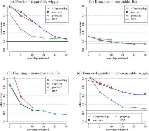
We consider four specific choices for the covariance: (a) a separable covariance with Fourier basis eigenfunctions and power decay of the eigenvalues; (b) Brownian sheet covariance, which is also separable; (c) the parametric covariance introduced by Gneiting (2002), which is nonseparable; and (d) a superposition of the Fourier covariance from (a) with another separable covariance, having shifted Legendre polynomial eigenfunctions and power decay of the eigenvalues. We discuss these choices in detail in Appendix I.4, supplementary materials. However, for the purpose of presenting the simulation results, it is only important to point out the following. First, while the Fourier setup (a) and the Brownian setup (b) are separable, the Gneiting setup (c) and the Fourier-Legendre setup (d) are nonseparable. Second, while the Brownian setup (b) and Gneiting setup (c) lead to rather flat covariances, the Fourier setup (a) and the Fourier-Legendre setup (d) lead to quite wiggly (though infinitely smooth) covariances.

Sparsity

In all simulation setups, we consider different percentages of the entries observed $p\in \{2,5,10,20,40,70\}$. Since the grid size is 20 × 20, this means for example, that for p = 2 we have $2/100·{20}^2=8$ observations per surface. For all the setups and percentages, we report relative estimation errors $\left|\right|\widehat{C}-C|{|}_2/|\left|C\right|{|}_2$, where $\widehat{C}$ is an estimator obtained by one of the four methods above (4D smoothing, one-step, proposed, or BSA). The results are shown in Figure 3. Every reported error was calculated as an average of 100 Monte Carlo runs.

Fig. 3 Relative estimation errors depending on percentages of the surfaces observed p for 4 ground truth covariance choices (a)–(d) and 4 methods compared. BSA provides a baseline, having access to full surfaces and hence not depending on p. For 4D smoothing, only results for small p are reported.

Error components

The reported estimation errors can be thought of having four components: (i) asymptotic bias, which is zero if the true covariance is separable, that is, in cases (a) and (b); (ii) error due to finite number of samples (N = 100); (iii) error due to sparse observations (i.e., not observing the full surfaces); and (iv) noise contribution. BSA errors are always free of the latter two, providing a baseline. The effect of not observing the full surfaces is displayed for different values of p. Finally, the noise contamination prevents smoothing approaches to reach the performance of BSA even for p large. Although our methodology explicitly handles noise, the finite sample performance is better with noise-free data, which only BSA has the access to.

Results

There is a number of comments to be made about the results in Figure 3:

1. In the setups where the covariance is flat, that is, (b) and (c), the one-step and the proposed approaches work the same, and 4D smoothing also works relatively well. These two setups are simple in a sense, because information can be borrowed quite efficiently via smoothing, regardless of whether the truth is separable or not. Still, the proposed approach using separability does not perform worse than 4D smoothing even in the nonseparable case (c), having the advantage of being much faster to obtain. For p = 10 the proposed estimator takes only a couple of seconds while 4D smoothing takes about 40 min even at this relatively small size of data.

2. When the true covariance is wiggly, the proposed methodology clearly outperforms 4D smoothing, both for the separable truth (a) and the nonseparable truth (d). The reason is that smoothing procedures are not very efficient in this case, and borrowing strength via separability is imperative.

3. The reason why error curves for 4D smoothing are only calculated up to p = 10 is the computational cost of smoothing in higher dimensions. In fact, performing 4D smoothing when p = 10 took more time than calculating of all the remaining results combined (cross-validations included). The runtimes are reported in Appendix I.5, supplementary materials.

Remark 1.

We used a standard cross-validation strategy to choose bandwidths for the separable model. However, for 4D smoothing, cross-validation is not feasible—using it would increase the total runtime of our simulation study to over 1000 CPU days. Therefore, we chose bandwidths for 4D smoothing based on those cross-validated for a separable model. This approach is taken throughout the article. See Appendices I.2 and I.5 for details and an empirical demonstration of the effectiveness of this choice.

5 Data Analysis: Implied Volatility Surfaces

A call option is a contract granting its holder the right, but not the obligation, to buy an underlying asset, for example, a stock, for an agreed-upon strike price at a defined expiration time. The ratio between the strike price and the current asset price is called moneyness, and the call option is traded for a certain market price $C^{*}(\hspace{0.17em}\text{log}\hspace{0.17em}(m),\tau )$, which depends on the moneyness m and the time to expiration τ. The Black–Sholes–Merton model (Black and Scholes 1973; Merton 1973) is commonly used to bijectively transform the observed market prices into implied volatilities, which can be thought of as an outlook of future fluctuations in the asset price. The advantage of considering the implied volatilities as opposed to the market prices of options themselves is that the implied volatilities tend to be smoother and comparable across different assets. Thus we can take advantage of the functional data analysis framework.

Since only certain combinations of the strike price and time to expiration are traded for a given asset, and these combinations differ across the assets, the implied volatility surfaces given as triplets of the moneyness, time to expiration and the corresponding implied volatility, that is $(m,\tau ,{\sigma }^{IV}(m,\tau ))$, can be treated as sparsely observed random surfaces. In this section, we consider the options data offered by DeltaNeutral (https://www.historicaloptiondata.com/content/free-data, retrieved on July 15, 2020), resulting in a dataset of N = 196 random surfaces. We take logarithms of moneyness and implied volatilities, and to reduce computational costs we round the log-moneyness and the time to expiration to fall on a common $50\times 50$ grid.

For details on implied volatilities and Black–Scholes–Merton model, as well as the data preprocessing steps, see Appendix I, supplementary materials.

Figure 4 shows two observations in our sample. The snapshot of Qualcomm Inc (QCOM) features a cummulation of observation at the short expiration. Here, it happens five times that two raw observations fall in the same pixel on the common 50 × 50 grid. In these few cases we calculate the average of the two observations in each pair. Due to smoothness, the option prices (and hence the implied volatilities) attain very similar values and thus this rounding and averaging does not change the conclusions of our analysis. We have observed this fact by fitting the model on finer grids while the estimates remained similar.

Fig. 4 Two sample snapshots of the considered log implied volatility surfaces corresponding to the call options on the stocks of Dell Technologies Inc on January 19, 2006 (a) and Qualcomm Inc on February 07, 2018 (b), and the mean surface of the implied volatility gained from pooling all the data together (c).

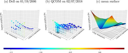
The estimated mean surface is displayed on the right-hand side of Figure 4. The mean surface captures the typical feature of the implied volatility surfaces: the volatility smile (Hull 2006). The implied volatility is typically greater for the options with moneyness away from 1, while this aspect is more significant for shorter times to expiration.

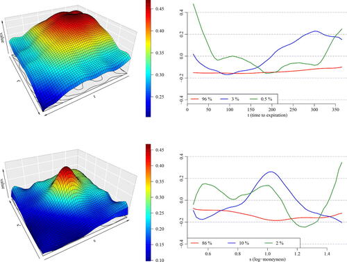
Figure 5 displays the estimates of the separable covariance components by our methodology presented in Section 2.3. The moneyness component demonstrates the highest marginal variability at the center of the covariance surface, meaning that the log implied volatility oscillates the most for the options with the log-moneyness around 0 (i.e., moneyness 1). The marginal variance is lower as the log-moneyness departs from 0. The eigendecomposition plot of the moneyness covariance kernel shows that the most of variability is explained by a nearly constant function with a small bump at the log-moneyness 0. The second leading eigenfunction adjusts the peak at the log-moneyness around 0 to a greater extent than the first eigenfunction. The covariance kernel corresponding to the time to expiration variable is smoother and demonstrates slightly higher marginal variability at shorter expiration. This phenomenon is well known for implied volatility (Hull 2006). The eigendecomposition of this covariance kernel indicates that the log implied volatility variation is mostly driven by the constant function while the second leading eigenfunction adjusts the slope of the surface for varying time to expiration.

Fig. 5 Top-left: The estimated covariance kernel $\widehat{a}=\widehat{a}(t,t\prime )$ corresponding to the time to expiration variable. Top-right: The three leading eigenfunctions of the spectral decomposition of the covariance kernel $\widehat{a}=\widehat{a}(t,t\prime )$. Bottom-left and botton-right: The same as above but for the estimated covariance kernel $\widehat{b}=\widehat{b}(s,s\prime )$ corresponding to the log-moneyness variable.

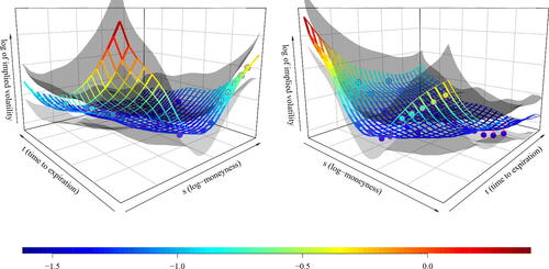
Figure 6 demonstrates our prediction techniques presented in Section 2.5 together with the 95% simultaneous prediction band. We recall that the prediction band aims to capture the latent smooth random surface itself, while our raw observations are modeled by adding an error term. Therefore, the raw data are not guaranteed to be covered in the band.

Fig. 6 Two views on prediction based on the call options written on the stock of Dell Technologies Inc on January 19, 2006. The circles depict the available sparse observations, the ribbons depict the predicted latent surface by the method of Section 2.5, where the covariance structure was assumed separable, and finally the transparent gray surfaces depict the 95% simultaneous prediction band for the latent log implied volatility surface.

5.1 Quantitative Comparison

The prediction method outlined in Section 2.5 requires as an input the pairwise covariances regardless whether they have been estimated by the separable estimator $\widehat{a}(t,t\prime )\widehat{b}(s,s\prime )$ or the 4D smoother $\widehat{c}(t,s,t\prime ,s\prime )$. As the benchmark for our comparison, we choose the locally linear kernel smoother (Fan and Gijbels 1996) applied individually for each surface as such smoothers constitute a usual preprocessing step (Cont and Da Fonseca 2002). We will refer to this predictor as pre-smoothing. In this section, we demonstrate that the predictive performance is comparable for both covariance estimator strategies (the separable and the 4D smoother), and that both of such approaches are superior to pre-smoothing. Moreover, the separable smoother is substantially faster than the 4D smoother.

We compare the prediction error by performing a 10-fold cross-validation, where the covariance structure is fitted always on varying 90% of the surfaces, with the remaining 10% used for out-of-sample prediction. In the set that is held out for prediction, we select some of the sparse observations and predict them based on the remaining observations on that surface. We use the following hold-out patterns:

1. Leave one chain out. Since the options are quotes always for a range of strikes, they constitute features known as option chains (see Figure 4) where multiple option prices (or equivalently implied volatilities) are available for a fixed time to expiration. For those surfaces that include at least two such chains, we remove gradually each chain and predict it based on the other chains. Therefore the number of prediction tasks performed on a single surface is equal to the number of chains observed per that surface.

2. Predict in-the-money. Predict implied volatilities for below-average moneyness (i.e., moneyness $m\le 1$) based on the out-of-the-money observations (moneyness m > 1).

3. Predict out-of-the-money. Predict implied volatilities for above-average moneyness (i.e., moneyness $m\ge 1$) based on the in-the-money observations (moneyness m < 1).

4. Predict short maturities. Predict the implied volatility for options with the time to maturity $\tau <183$ [days] based on the implied volatility of the options with the time to maturity $\tau \ge 183$ [days].

5. Predict long maturities. Predict the implied volatility for options with the time to maturity $\tau >183$ [days] based on the implied volatility of the options with the time to maturity $\tau \le 183$ [days].

All the prediction strategies are performed only for those surfaces where both the discarded part and the kept part are nonempty. We measure the prediction error on surface with the index n (in the test partition within the K-fold cross-validation) by the following root mean squared error (RMSE) criterion, relative to the pre-smoothing benchmark:(23) $$\sqrt{\mathrm{}\mathrm{}\frac{\sum _{m\in M_n^{\text{discarded}}}{\left(\mathrm{}({\widehat{\Pi }}^{\text{method}}(X(t_{nm},s_{nm})|{\mathbb{Y}}_n^{\text{kept}}))-Y_{nm}\mathrm{}\right)}^2}{\sum _{m\in M_n^{\text{discarded}}}{\left(\mathrm{}({\widehat{\Pi }}^{\text{pre}-\text{smooth}}(X(t_{nm},s_{nm})|{\mathbb{Y}}_n^{\text{kept}}))-Y_{nm}\mathrm{}\right)}^2}}$$(23) where $Y_{nm},m=1,\dots ,M_n$ are the implied volatility observations on the n-th surface, $M_n^{\text{discarded}}\subset \{1,\dots ,M_n\}$ denotes the set of observations’ indices discarded for the n-th surface, ${\mathbb{Y}}_n^{\text{kept}}$ are the vectorized implied volatility observations that were kept to be conditioned on. The predictor ${\Pi }^{\text{pre}-\text{smooth}}$ denotes the pre-smoothing based on the observations ${\mathbb{Y}}_n^{\text{kept}})$. The predictors ${\Pi }^{\text{method}}$ for method being either the separable smoother or the 4D smoother constitute the proposed predictors in this article with the covariance structure estimated by either of the two smoothers. These predictors are always trained only on the training partition (90% of the surfaces) within the 10-fold cross-validation scheme. Note that this out-of-sample comparison is adversarial for the proposed approach, because when predicting a fixed surface, the measurements on that surface (and another 10% of measurements total) are not used for the mean and covariance estimation. In practice, we naturally use all available information. However, for the hold-out comparison study here, that would require frequent refitting of the covariance, which would not be computationally feasible, in particular for 4D smoothing.

Figure 7 presents the results under the five hold-out patterns in form of boxplots created from the relative errors (23). We see that the prediction errors based on estimated covariances, be it the separable smoother or the 4D smoother, are typically smaller than the presmoothing benchmark with the only exception of the 4D smoother in the hold-out pattern (b). The predictive performances of the separable and the 4D smoother are comparable, but they differ a lot in terms of runtime. It typically takes 30 seconds to calculate the separable smoother (including a cross-validation based selection of the smoothing bandwidths), while the 4D smoother takes around 3 hr. The latter runtime is moreover without considering any automatic selection of the bandwidths, because such would be computationally infeasible. Hence we use the bandwidths selected by the separable model, as described in Remark 1. The calculations are performed on a quite coarse grid of size 20 × 20. The calculations on a dense grid, such as 50 × 50 used in the qualitative analysis in Section 5 are not feasible for the 4D smoother.

Fig. 7 Boxplots of root mean squared errors relative to the pre-smoothing benchmark (23) for prediction method of Section 2.5 with the covariance estimated by 4D smoothing or the proposed separable approach, and different hold-out patterns: (a) leave one chain out; (b) predict in-the-money; (c) predict out-of-the-money; (d) predict short maturities; and (e) predict long-maturities. Numbers inside the boxes provide numerical values of the median. For a given method, RMSE value 3 means that the given method is 3-times worse than the benchmark, while RMSE value 1/3 corresponds to 3-fold improvement.

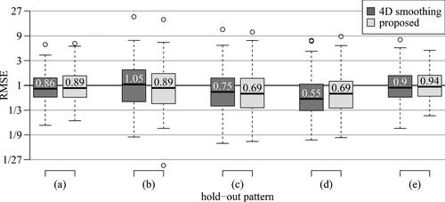
Therefore we conclude that the separable smoother approach enjoys a better predictive performance than the pre-smoothing benchmark and—while having similar predictive performance as the predictor based on 4D smoothing—is computationally much faster than the said competitor. In fact, it requires two-dimensional smoothers only, just as the pre-smoothing benchmark.

6 Conclusions and Future Directions

In practice, covariances are often nonseparable (Gneiting, Genton, and Guttorp 2006; Aston, Pigoli, and Tavakoli 2017; Bagchi and Dette 2020; Dette, Dierickx, and Kutta 2020; Pigoli et al. 2018; Rougier 2017), and assuming separability induces a bias. The variance stemming from sparse measurements and noise contamination is, however, often of a of larger magnitude, thus sanctioning separability as a means to achieve a better bias-variance tradeoff. Moreover, separability entails faster computation and lower storage requirements. As demonstrated above, these advantages are pronounced in the sparse regime.

When data are observed fully and no smoothing is used (i.e., simple averages are calculated at the grid points instead), calculation of the estimator takes about 0.03 sec in case of separability and 0.12 sec in general, with our grid size 20 and sample size N = 100. With larger grid size, the acceleration gained by assuming separability naturally magnifies. But still, separability is assumed mostly to save memory rather than time, in the fully observed case (Aston, Pigoli, and Tavakoli 2017). On the other hand, with sparsely observed data and kernel smoothing deployed, the speed-up factor stemming from separability can be of the order of hundreds already with rather small grid sizes. The point we advocate is that—with sparse observations, kernel smoothing deployed, and compared to observations on a grid—the computational savings offered by separability are the same in terms of memory, but are much more profound in terms of runtime. This is due to the extra costs associated with smoothing.

Our analysis of implied volatility surfaces provides some insights into the statistical dependencies of such sparsely observed data, and our quantitative comparison demonstrates how the proposed prediction method outperforms the pre-smoothing benchmark. We have formed our dataset collecting options across various symbols and timestamps with the reasoning that the volatility across these come also from one population, which is debatable. This study should be seen rather as a proof-of-concept on how to “borrow strength” across the dataset, and how this approach can be used to decrease the prediction error.

Having said that, we believe that our methodology can provide even better results when considering a more homogeneous population such as the time series of the implied volatility surfaces related to a single fixed symbol/asset. In this case, pre-smoothing is usually required (Cont and Da Fonseca 2002; Kearney, Cummins, and Murphy 2018) for forecasting of such time series. Our methodology could avoid the pre-smoothing step in this case by predicting the surfaces while borrowing the information across the entire dataset. Furthermore, our methodology could be easily tailored to predicting principal components scores by conditional expectation (similarly to Yao, Müller, and Wang 2005), which could be used for forecasting by a vector autoregression. Combining separable covariances and time series of sparsely observed surfaces hints at other directions of future work. For example, Rubín and Panaretos (2020) showed how to estimate the spectral density operator nonparametrically from sparsely observed functional time series. Estimating separable spectral density operator for sparsely observed surface-valued time series seems to be within reach and is likely to provide predictions that benefit from the information across time, and thus, reducing the prediction error even more.

While our methodology is aimed at sparsely observed surfaces, it can be also used for unbalanced regimes, where some surfaces are observed only at few locations while others at many more. It is natural to ask whether an additional “per-subject” weighting scheme such as the one proposed by Li and Hsing (2010) could be generalized to the multi-dimensional case and lead to a better performance. The motivation here is to take into account different levels of information contained in a single point on a sparsely observed surface compared to a single point on a densely observed surface. We provide a detailed discussion of this direction in Appendix III, supplementary materials.

Acknowledgments

The authors thank the editor, the associate editor, and two anonymous referees for their valuable feedback.

Supplementary Materials

Appendix:The Appendix contains all the proofs and some additional results, as referenced from the main paper. (appendix.pdf)

R code:The available R code implements the methodology proposed in the main paper, and can be used to reproduce the reported results. (see README.txt)

Additional information

Funding

This research was supported by a Swiss National Science Foundation grant.

References

- Aston, J. A., Pigoli, D., and Tavakoli, S. (2017), “Tests for Separability in Nonparametric Covariance Operators of Random Surfaces,” The Annals of Statistics, 45, 1431–1461. DOI: 10.1214/16-AOS1495.
- Bagchi, P., and Dette, H. (2020), “A Test for Separability in Covariance Operators of Random Surfaces,” Annals of Statistics, 48, 2302–2322.
- Black, F., and Scholes, M. (1973), “The Pricing of Options and Corporate Liabilities,” Journal of Political Economy, 81, 637–654. DOI: 10.1086/260062.
- Chen, L.-H., and Jiang, C.-R. (2017), “Multi-Dimensional Functional Principal Component Analysis,” Statistics and Computing, 27, 1181–1192. DOI: 10.1007/s11222-016-9679-5.
- Constantinou, P., Kokoszka, P., and Reimherr, M. (2017), “Testing Separability of Space-Time Functional Processes,” Biometrika, 104, 425–437.
- Cont, R., and Da Fonseca, J. (2002), “Dynamics of Implied Volatility Surfaces,” Quantitative Finance, 2, 45–60. DOI: 10.1088/1469-7688/2/1/304.
- De Iaco, S., Myers, D. E., and Posa, D. (2002), “Nonseparable Space-Time Covariance Models: Some Parametric Families,” Mathematical Geology, 34, 23–42. DOI: 10.1023/A:1014075310344.
- Degras, D. A. (2011), “Simultaneous Confidence Bands for Nonparametric Regression with Functional Data,” Statistica Sinica, 21, 1735–1765. DOI: 10.5705/ss.2009.207.
- Dette, H., Dierickx, G., and Kutta, T. (2020), “Quantifying Deviations from Separability in Space-Time Functional Processes,” arXiv preprint arXiv:2003.12126.
- Fan, J., and Gijbels, I. (1996), Local Polynomial Modelling and Its Applications: Monographs on Statistics and Applied Probability (Vol. 66), Boca Raton, FL: CRC Press.
- Fengler, M. R. (2009), “Arbitrage-Free Smoothing of the Implied Volatility Surface,” Quantitative Finance, 9, 417–428. DOI: 10.1080/14697680802595585.
- Genton, M. G. (2007), “Separable Approximations of Space-Time Covariance Matrices,” Environmetrics: The Official Journal of the International Environmetrics Society, 18, 681–695. DOI: 10.1002/env.854.
- Gneiting, T. (2002), “Nonseparable, Stationary Covariance Functions for Space–Time Data,” Journal of the American Statistical Association, 97, 590–600. DOI: 10.1198/016214502760047113.
- Gneiting, T., Genton, M. G., and Guttorp, P. (2006), Geostatistical Space-Time Models, Stationarity, Separability, and Full Symmetry, Boca Raton, FL: Chapman and Hall/CRC, pp. 151–175.
- Hall, P., Müller, H.-G., and Wang, J.-L. (2006), “Properties of Principal Component Methods for Functional and Longitudinal Data Analysis,” The Annals of Statistics, 34, 1493–1517. DOI: 10.1214/009053606000000272.
- Henderson, C. R. (1975), “Best Linear Unbiased Estimation and Prediction Under a Selection Model,” Biometrics, 31, 423–447. DOI: 10.2307/2529430.
- Hull, J. (2006), Options, Futures, and Other Derivatives (Pearson International ed.), New York: Pearson/Prentice Hall.
- Kearney, F., Cummins, M., and Murphy, F. (2018), “Forecasting Implied Volatility in Foreign Exchange Markets: A Functional Time Series Approach,” The European Journal of Finance, 24, 1–18. DOI: 10.1080/1351847X.2016.1271441.
- Li, Y., and Hsing, T. (2010), “Uniform Convergence Rates for Nonparametric Regression and Principal Component Analysis in Functional/Longitudinal Data,” The Annals of Statistics, 38, 3321–3351. DOI: 10.1214/10-AOS813.
- Lopez, G., Eisenberg, D. P., Gregory, M. D., Ianni, A. M., Grogans, S. E., Masdeu, J. C., Kim, J., Groden, C., Sidransky, E., and Berman, K. F. (2020), “Longitudinal Positron Emission Tomography of Dopamine Synthesis in Subjects with gba1 Mutations,” Annals of Neurology, 87, 652–657. DOI: 10.1002/ana.25692.
- Masak, T., and Panaretos, V. M. (2019), “Spatiotemporal Covariance Estimation by Shifted Partial Tracing,” arXiv preprint arXiv:1912.12870.
- Masak, T., Sarkar, S., and Panaretos, V. M. (2020), “Principal Separable Component Analysis via the Partial Inner Product,” arXiv preprint arXiv:2007.12175.
- Merton, R. C. (1973), “Theory of Rational Option Pricing,” The Bell Journal of Economics and Management Science, 4, 141–183. DOI: 10.2307/3003143.
- Pigoli, D., Hadjipantelis, P. Z., Coleman, J. S., and Aston, J. A. (2018), “The Statistical Analysis of Acoustic Phonetic Data: Exploring Differences Between Spoken Romance Languages,” Journal of the Royal Statistical Society, Series C, 67, 1103–1145. DOI: 10.1111/rssc.12258.
- Ramsay, J., and Silverman, B. (2007), Applied Functional Data Analysis: Methods and Case Studies, Springer Series in Statistics, New York: Springer.
- Ramsay, J. O., and Silverman, B. W. (2005), Functional Data Analysis, New York: Springer.
- Rougier, J. (2017), “A Representation Theorem for Stochastic Processes with Separable Covariance Functions, and Its Implications for Emulation,” arXiv preprint arXiv:1702.05599.
- Rubín, T., and Panaretos, V. M. (2020), “Sparsely Observed Functional Time Series: Estimation and Prediction,” Electronic Journal of Statistics, 14, 1137–1210. DOI: 10.1214/20-EJS1690.
- Wang, J., Wong, R. K., and Zhang, X. (2020), “Low-Rank Covariance Function Estimation for Multidimensional Functional Data,” Journal of the American Statistical Association, 1–14. DOI: 10.1080/01621459.2020.1820344.
- Yao, F., Müller, H.-G., and Wang, J.-L. (2005), “Functional Data Analysis for Sparse Longitudinal Data,” Journal of the American Statistical Association, 100, 577–590. DOI: 10.1198/016214504000001745.
- Yarger, D., Stoev, S., and Hsing, T. (2020), “A Functional-Data Approach to the Argo Data,” arXiv preprint arXiv:2006.05020.
- Zhang, H., and Li, Y. (2020), “Unified Principal Component Analysis for Sparse and Dense Functional Data Under Spatial Dependency,” arXiv preprint arXiv:2006.13489.
- Zhang, X., and Wang, J.-L. (2016), “From Sparse to Dense Functional Data and Beyond,” The Annals of Statistics, 44, 2281–2321. DOI: 10.1214/16-AOS1446.