Connecting the Dots: Numerical Randomized Hamiltonian Monte Carlo with State-Dependent Event Rates

Abstract

Numerical generalized randomized Hamiltonian Monte Carlo is introduced, as a robust, easy to use and computationally fast alternative to conventional Markov chain Monte Carlo methods for continuous target distributions. A wide class of piecewise deterministic Markov processes generalizing Randomized HMC (Bou-Rabee and Sanz-Serna) by allowing for state-dependent event rates is defined. Under very mild restrictions, such processes will have the desired target distribution as an invariant distribution. Second, the numerical implementation of such processes, based on adaptive numerical integration of second order ordinary differential equations (ODEs) is considered. The numerical implementation yields an approximate, yet highly robust algorithm that, unlike conventional Hamiltonian Monte Carlo, enables the exploitation of the complete Hamiltonian trajectories (hence, the title). The proposed algorithm may yield large speedups and improvements in stability relative to relevant benchmarks, while incurring numerical biases that are negligible relative to the overall Monte Carlo errors. Granted access to a high-quality ODE code, the proposed methodology is both easy to implement and use, even for highly challenging and high-dimensional target distributions. Supplementary materials for this article are available online.

KEYWORDS:

• Hamiltonian Monte Carlo
• MCMC
• Piecewise deterministic processes
• Runge-Kutta-Nystrom

1 Introduction

By now, Markov chain Monte Carlo (MCMC) methods and their widespread application in Bayesian statistics need no further introduction (see, e.g., Robert and Casella 2004; Gelman et al. 2014). In this article, Generalized Randomized Hamiltonian Monte Carlo (GRHMC), a wide class of continuous time Markov processes with a preselected stationary distribution is constructed. Further, Numerical GRHMC (NGRHMC), the practical implementation of GRHMC processes is suggested as a robust and easy to use general purpose class of algorithms for solving problems otherwise handled using MCMC methods for continuous state spaces.

The article makes several contributions. GRHMC processes, a wide class of piecewise deterministic Markov processes (PDMP) (see, e.g., Davis 1993; Fearnhead et al. 2018; Vanetti et al. 2018, and references therein) with target distribution-preserving Hamiltonian deterministic dynamics are defined. GRHMC processes generalizes Randomized HMC (Bou-Rabee and Sanz-Serna 2017) by admitting state-dependent event-rates, while still retaining arbitrary prespecified stationary distributions. The highly flexible specification of event rates leaves substantial room to construct processes that are more optimized toward MCMC applications. A further benefit of using conserving Hamiltonian deterministic dynamics is that GRHMC processes are likely to scale well to high-dimensional problems (see, e.g., Bou-Rabee and Eberle 2020 where dimension-free convergence bounds are obtained for the Anderson Thermostat, which generalizes RHMC).

Second, it is proposed to use adaptive numerical methods for second order ordinary differential equations (ODEs) (see, e.g., Hairer, Nørsett, and Wanner 1993) to approximate a selected GRHMC process to arbitrary precision, leading to NGRHMC. In common implementations of Hamiltonian Monte Carlo, errors introduced by fixed time step (i.e., nonadaptive) symplectic/time-reversible integrators are exactly corrected using accept/reject steps. Here, biases relative to the (on target, but generally intractable) GRHMC process stemming from the numerical integration of ODEs are not explicitly corrected for, but rather kept under control by choosing the ODE integrator precision sufficiently high. Numerical experiments indicate that even for rather lax integrator precision, biases incurred by the numerical integration of ODEs are imperceivable relative to the overall Monte Carlo variation stemming from using MCMC-like methods.

By allowing for such small biases, one may leverage high-quality adaptive ODE integration codes, making the proposed method both easy to implement and requiring minimal expertise by the user. The system of ODEs may be augmented beyond Hamilton’s equations so that sampling of event times under nontrivial event rates (without specifying model-specific bounds on the event rates (Fearnhead et al. 2018) and computing averages over continuous time trajectories are done within ODE solver. This practice of augmenting the ODE system ensures that the precision of the overall algorithm (including the simulation of event times and computation of moments) relative to the underlying GRHMC process is controlled by a single error control mechanism and only a few easily interpretable tuning parameters. Automatic tuning methodology of the parameters in underlying GRHMC process, again leveraging aspects of the adaptive ODE integration code, is also proposed.

Third, it is demonstrated that certain moments of the target distribution may be estimated extremely efficiently by exploiting the between events Hamiltonian dynamics (and hence the name of the article). Such improved efficiency occur when the temporal averages of the position coordinate of the Hamiltonian trajectories (without momentum refreshes) coincide with the corresponding means under the target distributions. Such effects occurs for example, when estimating the mean under Gaussian target distributions, but is by no means restricted to this situation. Exploitation of any such effects is straight forward when the theoretical processes are approximated using ODE solvers as proposed.

Finally, it is demonstrated that even rudimentary versions of NGRHMC have competitive performance compared to commonly used (fixed time step) symplectic/time-reversible methods for target distributions where the latter methods work well. Furthermore, it is demonstrated that adaptive nature of the integrators employed here resolves the slow exploration associated with fixed step size HMC-MCMC chains for target distributions exhibiting certain types of nonlinearities.

This article, contains only initial steps toward understanding and exploiting the full potential of GRHMC processes and their numerical implementation and should be read as an invitation to further work. On the theoretical side, understanding the ergodicity of GRHMC processes beyond RHMC, bounding the biases stemming from numerical integration and understanding scaling in high dimensions would be natural next steps. Better exploiting the possibilities afforded by the highly flexible state-dependent event rates constitutes another major avenue for further work. Throughout the text, further suggestions for continued research in several other regards are also pointed out.

1.1 Relation to Other Work

Continuous time Markov processes involving Hamiltonian dynamics subject to random updates of velocities at random times are by no means new. In the molecular simulation literature, the Anderson Thermostat (AT) (Andersen 1980) involves Hamiltonian dynamics with updating of the momentum of randomly chosen particles according to Bolzmann-Gibbs distribution marginals. RHMC may be seen as a special case of the AT with only one particle (Bou-Rabee and Eberle 2020). Uncorrected numerical implementations of the AT, involving fixed time step reversible integrators may be found in several molecular simulation packages such as GROMACS (Abraham et al. 2015).

The theoretical properties of the RHMC (with constant event rate and exact Hamiltonian dynamics) and AT have been extensively studied: Bou-Rabee and Sanz-Serna (2017) develop geometric ergodicity of RHMC under mild assumptions. Further, E and Li (2008) and Li (2007) develop ergodicity for both continuous time AT and its time-discretization under different assumptions, and Bou-Rabee and Eberle (2020) consider the convergence of AT in Wasserstein distance. Lu and Wang (2020) study RHMC under the hypocoercivity framework. As described by Bou-Rabee and Sanz-Serna (2017), there is also an interesting and fundamental connection between RHMC and second-order Langevin dynamics (see, e.g., Cheng et al. 2018, and references therein) in that the same stochastic Lyapunov function may be used to prove geometric ergodicity of both types of processes.

Recently, PDMPs (see, e.g., Davis 1993; Fearnhead et al. 2018; Vanetti et al. 2018, and references therein) have received substantial interest as time-irreversible alternatives to conventional MCMC methods. Most proposed PDMP-based alternatives to MCMC, such as the Bouncy Particle Sampler (Bouchard-Côté, Vollmer, and Doucet 2018) and the Zig-Zag process (Bierkens, Fearnhead, and Roberts 2019) rely on linear deterministic dynamics. Another PDMP-based sampling algorithm; The Boomerang Sampler (BS) (Bierkens et al. 2020) uses the explicitly solvable Hamiltonian deterministic dynamics associated with Gaussian approximation to the target. The BS was found to outperform the mentioned linear dynamics PDMPs. AT, RHMC along with GRHMC are also PDMPs based on Hamiltonian deterministic dynamics, but unlike the BS, the involved deterministic dynamics preserves exactly the target distribution, hence, affording GRHMC substantial flexibility with respect to the selection of event rates. Interestingly, Deligiannidis et al. (2018) shows that the RHMC process is a scaling limit of the Bouncy Particle Sampler (Bouchard-Côté, Vollmer, and Doucet 2018). RHMC processes (i.e., with exact Hamiltonian dynamics and constant event rates) are also mentioned in the context of PDMPs by (Vanetti et al. 2018, footnote 3), but no details are provided on how to implement such an algorithm are provided.

Inter-event time sampling for PDMPs based on numerical integration and root-finding (and thereby bypassing the need for global bounds on the event rate as is also done in this article) is considered by Cotter, House, and Pagani (2020). However, their approach is based on the linear Zig-Zag dynamics and uses other numerical techniques to obtain integrated event rates. HMC-MCMC based on exact Hamiltonian dynamics is considered by Pakman and Paninski (2014), but their approach is restricted to truncated Gaussian distributions where such dynamics may be found on closed form. Theoretical work for HMC-MCMC assuming exact target-preserving Hamiltonian dynamics may be found in for example, Mangoubi and Smith (2017) and Chen and Vempala (2019). Nishimura and Dunson (2020) consider recycling the intermediate integrator-steps in HMC-MCMC in a manner related to the temporal averages considered here, and also find substantial improvements in simulation efficiency in numerical experiments.

Unadjusted (and therefore generally biased) numerical approximations to intractable theoretical processes for simulation purposes have received much attention, with the widely used stochastic gradient Langevin dynamics (Welling and Teh 2011) being such an example. In particular, both first- and second order Langevin dynamics, along with their multiple integration step counterpart, generalized HMC (Horowitz 1991), have been implemented in unadjusted manners (see, e.g., Leimkuhler and Matthews 2015, for an overview). In addition, several theoretical papers consider unadjusted HMC-MCMC algorithms, see, for example, Mangoubi and Smith (2019), Bou-Rabee and Schuh (2020) and Bou-Rabee and Eberle (2021). In this strand of literature, also so-called collocation methods (which are closely related to certain Runge Kutta methods (Hairer, Nørsett, and Wanner 1993) are applied by Lee, Song, and Vempala (2018) for solving Hamilton’s equations, but their approach is again based on (discrete time-)HMC-MCMC and does not appear to leverage modern numerical ODE techniques. Finally, the present use of adaptive step size techniques has similarities to Kleppe (2016), but the latter algorithm is based on Langevin processes and involves a Metropolis–Hastings adjustment step.

The reminder of this article is laid out as follows: Section 2 provides background and fixes notation. GRHMC processes are defined and discussed in Section 3. The practical numerical implementation of such processes is discussed in Section 4. Numerical experiments and illustrations, along with benchmarks against Stan are given in Sections 5 and 6. Finally, Section 7 provides discussion. The complete set of source code underlying this article is available at https://github.com/torekleppe/PDPHMCpaperCode.

2 Background

This section provides some background and fixes notation for subsequent use. Throughout this article, a target distribution with density $\pi (\mathit{q}),\mathit{q}\in \Omega \subseteq {\mathbb{R}}^d$ with an associated density kernel $\tilde{\pi }(\mathit{q})$ which can be evaluated point-wise. The gradient/Jacobian operator of a function with respect to some variable, say x, is denoted by ${\nabla }_{\mathit{x}}$. Time-derivatives are denoted using the conventional dot-notation, that is, $\dot{f}(\tau )=\frac{d}{d\tau }f(\tau ),$ $\ddot{f}(\tau )=\frac{d^2}{d{\tau }^2}f(\tau )$ for some function $f(\tau )$ evolving over time τ.

In the reminder of this section, Hamiltonian mechanics, HMC and PDMPs are briefly reviewed in order to fix notation and provide the required background. The reader is referred to Goldstein, Poole, and Safko (2002), Leimkuhler and Reich (2004), Neal (2010), and Bou-Rabee and Sanz-Serna (2018) for more detailed expositions of Hamiltonian mechanics and HMC. Davis (1984, 1993) for consider PDMPs in general and Fearnhead et al. (2018) and Vanetti et al. (2018) give details for Monte Carlo applications of PDMPs.

2.1 Elements of Hamiltonian Mechanics

Hamiltonian Monte Carlo methods rely on specifying a physical system and use the dynamics of this system to propose transitions. The state $\mathit{z}={[{\mathit{q}}^T,{\mathit{p}}^T]}^T\in {\mathbb{R}}^{2d}$ of the system is characterized by a position coordinate $\mathit{q}\in {\mathbb{R}}^d$ and a momentum coordinate $\mathit{p}\in {\mathbb{R}}^d$. The system itself is conventionally specified in terms of the Hamiltonian $\mathcal{H}(\mathit{z})=\mathcal{H}(\mathit{q},\mathit{p})$ which gives the total energy of the system for a given state z. Throughout this work, physical systems with Hamiltonian given as(1) $$\mathcal{H}(\mathit{q},\mathit{p})=-\hspace{0.17em}\text{log}\hspace{0.17em}\tilde{\pi }(\mathit{q})+\frac{1}{2}{\mathit{p}}^T{\mathit{M}}^{-1}\mathit{p},$$(1) are considered. Here $\mathit{M}\in {\mathbb{R}}^{d\times d}$ is a symmetric, positive definite (SPD) mass matrix which is otherwise specified freely. The time-evolution of the system is given by Hamilton’s equations $\stackrel{.}{\mathit{q}}(\tau )={\nabla }_{\mathit{p}}\mathcal{H}(\mathit{q}(\tau ),\mathit{p}(\tau )),$ $\stackrel{.}{\mathit{p}}(\tau )=-{\nabla }_{\mathit{q}}\mathcal{H}(\mathit{q}(\tau ),\mathit{p}(\tau ))$, which for Hamiltonian (1) reduces to:(2) $$\stackrel{.}{\mathit{z}}(\tau )=\left[\begin{array}{c}\stackrel{.}{\mathit{q}}(\tau )\\ \stackrel{.}{\mathit{p}}(\tau )\end{array}\right]=\left[\begin{array}{c}{\mathit{M}}^{-1}\mathit{p}(\tau )\\ {\nabla }_{\mathit{q}}\hspace{0.17em}\text{log}\hspace{0.17em}\tilde{\pi }(\mathit{q}(\tau ))\end{array}\right].$$(2)

The flow associated with (2) is denoted by ${\phi }_{\tau }(·)$, and is defined so that $\mathit{z}(\tau +s)={\phi }_s(\mathit{z}(\tau ))$ solves (2) for any scalar time increment s, initial time τ and initial configuration $\mathit{z}(\tau )$. The flow can be shown to be

• Energy preserving, that is, $\frac{\partial }{\partial \tau }\mathcal{H}({\phi }_{\tau }(\mathit{z}))=0$ for all admissible z;

• volume preserving, that is, $|{\nabla }_{\mathit{z}}{\phi }_{\tau }(\mathit{z})|=1$ for each fixed τ and all admissible z;

• time reversible, which in the present context is most conveniently formulated via that ${\mathit{T}}_{\tau }=\mathit{R}°{\phi }_{\tau }$ is an involution so that ${\mathit{T}}_{\tau }°{\mathit{T}}_{\tau }$ is the identity operator. The momentum flip operator $\mathit{R}=\text{diag}({\mathit{I}}_d,-{\mathit{I}}_d)$ effectively reverses time.

2.2 Hamiltonian Monte Carlo

In the context of statistical computing, Hamiltonian dynamics has attracted much attention the last decade. This interest is rooted in that the flow ${\phi }_{\tau }$ of (2) (and associated involution ${\mathit{T}}_{\tau }$) exactly preserves the Boltzmann-Gibbs (BG) distribution(3) $$\rho (\mathit{z})=\rho (\mathit{q},\mathit{p})=\pi (\mathit{q})\mathcal{N}(\mathit{p}|{\mathbf{0}}_d,\mathit{M})\propto \hspace{0.17em}\text{exp}\hspace{0.17em}(-\mathcal{H}(\mathit{q},\mathit{p})),$$(3) associated with $\mathcal{H}$. That is, for each fixed time increment τ, ${\phi }_{\tau }(\mathit{z})$ $\sim \rho$ whenever $\mathit{z}\sim \rho$. It is seen that the target distribution is the q-marginal of the BG distribution. Thus, a hypothetical MCMC algorithm targeting (3), and producing samples ${\mathit{z}}_{(i)}={({\mathit{q}}_{(i)}^T,{\mathit{p}}_{(i)}^T)}^T$, would involve the BG distribution-preserving steps:

• Sample ${\mathit{p}}_{*}\sim N(\varphi {\mathit{p}}_{(i-1)},\sqrt{1-{\varphi }^2}\mathit{M})$ for some $\varphi \in (-1,1)$ and set ${\mathit{z}}_{*}={({\mathit{q}}_{(i-1)}^T,{\mathit{p}}_{*}^T)}^T$.

• For some suitable time increment s, ${\mathit{z}}_{(i)}={\phi }_s({\mathit{z}}_{*})$.

Subsequently, the momentum samples, ${\mathit{p}}_{(i)}$, may be discarded to obtain samples targeting $\pi (\mathit{q})$ only. Randomized durations s may be introduced in order to avoid periodicities or near-periodicities in the underlying dynamics, and may result in faster convergence (Mackenze 1989; Cances, Legoll, and Stoltz 2007; Bou-Rabee and Sanz-Serna 2017, 2018). Alternatively, more sophisticated algorithms can be used to avoid u-turns (Hoffman and Gelman 2014).

For all but the most analytically tractable target distributions, the flow associated with Hamilton’s equations is not available in closed form, and hence it must be integrated numerically for the practical implementation of the above MCMC sampler. Provided a time-reversible integrator is employed for this task, the numerical error incurred in the second step of the above MCMC algorithm can be exactly corrected using an accept/reject step (Fang, Sanz-Serna, and Skeel 2014), but the accept probability may be computationally demanding. If the employed integrator is also volume preserving (i.e., symplectic) (see, e.g., Leimkuhler and Reich 2004), the accept-probability depends only on the values of the Hamiltonian before and after the integration. This simplification has led to the widespread application of the symplectic leap-frog (or Størmer-Verlet) integrator in HMC implementations such as for example, Stan (Stan Development Team 2017).

Requiring the integrator to be time reversible and symplectic imposes rather strict restrictions on the integration process. In particular the application of adaptive (time-)step sizes, which is an integral part of any modern general purpose numerical ODE code, is at best difficult to implement (see Leimkuhler and Reich 2004, chap. 9 for discussion of this problem) while maintaining time-reversible and symplectic properties.

Figure 1 illustrates the effect of using fixed step sizes for the funnel-type distribution $q_1\sim N(0,1),q_2|q_1\sim N(0,\hspace{0.17em}\text{exp}\hspace{0.17em}(3q_1))$ (further details on this experiment can be found in Section 5.1). In the four left panels, empirical cumulative distribution functions (CDFs) calculated from MCMC output using the fixed step size integrator in Stan are depicted for various accept rate targets δ which has a default value of 0.8. In practice, higher values of δ correspond to higher fidelity integration with smaller integrator step sizes and more integrator steps per produced sample. It is seen that even with very small step sizes, Stan fails to properly represent the left-hand tail of q₁ (which imply a very small scale in the q₂). In the $\delta =0.999$ case, the smallest produced sample out 50,000 is $\approx -3.026$. In an iid N(0, 1) sample of this size, one would expect around 62 samples smaller than this value.

Fig. 1 Empirical cumulative distribution functions (CDFs) associated with MCMC output for the standard Gaussian ${\mathit{q}}_1$-marginal under the “funnel”-model ${\mathit{q}}_1\sim N(0,1)$, ${\mathit{q}}_2|{\mathit{q}}_1\sim N(0,\hspace{0.17em}\text{exp}\hspace{0.17em}(3{\mathit{q}}_1))$. For visual clarity, only the left half of the distributions are presented. Further details on this experiment can be found in Section 5.1. Each case is based on 5000 samples from each of 10 independent replica. The black solid lines are the empirical CDFs, whereas the red dashed lines are the true CDFs. The shaded gray region would cover 90% of empirical CDFs based on 50,000 iid N(0, 1) samples point-wise. The four left-most panels are based on Stan output with different values of the accept rate target δ. In practice, higher values of δ corresponds to smaller integrator step sizes and more integrator steps per produced sample. The right-most panel shows output for the proposed methodology using constant event rates. For both Stan and the proposed methodology, an identity mass matrix was employed.

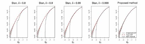
Also included in Figure 1 are results from a variant of the proposed methodology (see Section 5.1 for details), which is based on adaptive numerical integrators. The method shows no such pathologies, and in particular the number of samples below the smallest $\delta =0.999$ Stan sample was 70.

2.3 Piecewise Deterministic Markov Processes

Recently, continuous time piecewise deterministic Markov processes (PDMP) (see, e.g., Davis 1984, 1993) have been considered as alternatives to discrete time Markov chains produced by conventional MCMC methods. PDMPs may be employed for simulating dependent samples, or more generally continuous time trajectories with a given marginal probability distribution (see Fearnhead et al. 2018, and references therein). As the name indicates, PDMPs follow a deterministic trajectory between events occurring at stochastic times. At events, the state is updated in a stochastic manner.

Following Fearnhead et al. (2018), a PDMP, say $\mathcal{Z}(t)\in {\mathbb{R}}^D$, $t\in [0,\infty )$, is specified in terms of three components $(\Phi ,\lambda ,Q)$:

• Deterministic dynamics on time intervals where events do not occur, specified in terms of a set of ODEs: $\stackrel{.}{\mathcal{Z}}(t)=\Phi (\mathcal{Z}(t))$.

• A nonnegative event rate $\lambda (\mathcal{Z}(t))$, depending only on the current state of the process, so that the probability of an event between times t and t + r, $r\ge 0$ is $\lambda (\mathcal{Z}(t))r+o(r)$ for small r.

• Finally, a “transition distribution at events” $Q(·|\mathcal{Z}(t-))$. Suppose an event occurs at time t, and $\mathcal{Z}(t-)$ is the state immediately before time t. Then the $\mathcal{Z}(t)$ will be drawn randomly with density $Q(·|\mathcal{Z}(t-))$.

Let Ξ_s be the flow associated with $\Phi$. In order to simulate from a PDMP, suppose first that $\mathcal{Z}(0)$ has been set to some value, and that t is initially set to zero. Then the following three steps are repeated until $t>T$ where T is the desired length of the PDMP trajectory:

• Simulate a new $u\sim$ Exp(1) and subsequently compute the time-increment until next event v, which obtains as the solution in v to(4) $$\Lambda (v;\mathcal{Z}(t))=u,\text{where}\mathrm{}\Lambda (v;\mathit{z})={\int }_0^v\lambda ({\Xi }_s(\mathcal{Z}(t)))ds.$$(4)

• Set $\mathcal{Z}(t+s)={\Xi }_s(\mathcal{Z}(t))$ for all $s\in [0,v)$, and ${\mathcal{Z}}^{*}={\Xi }_v(\mathcal{Z}(t))$.

• Set $t\leftarrow t+v$ and simulate $\mathcal{Z}(t)\sim Q(·|{\mathcal{Z}}^{*})$.

An invariant distribution of the process $\mathcal{Z}(t)$, say $p(\mathit{z})$, will satisfy the time-invariant Fokker-Planck/Kolmogorov forward equation (Fearnhead et al. 2018)(5) $$\sum _{i=1}^D\frac{\partial }{\partial z_i}\left[{\Phi }_i(\mathit{z})p(\mathit{z})\right]=\int p({\mathit{z}}^{\prime })\lambda ({\mathit{z}}^{\prime })Q(\mathit{z}|{\mathit{z}}^{\prime })d{\mathit{z}}^{\prime }-p(\mathit{z})\lambda (\mathit{z}),$$(5) for all admissible states z. For continuous time Monte Carlo applications, one therefore, seeks combinations of $(\Phi ,\lambda ,Q)$ so that the desired target distribution is an invariant distribution $p(\mathit{z})$.

Provided such a combination has been found, discrete time Markovian samples(6) $${\mathit{z}}_{(i)}=\mathcal{Z}(\Delta i),\text{for}\mathrm{}\text{some}\mathrm{}\text{sample}\mathrm{}\text{spacing}\mathrm{}\Delta >0,$$(6) may be used in the same manner as regular MCMC samples for characterizing the invariant distribution. In addition, by letting the sample spacing $\Delta \to 0$, moments under the invariant distribution may also be obtained by using the complete trajectory of the PDMP, that is,(7) $$\frac{1}{T}{\int }_0^{T}g(\mathcal{Z}(t))dt\underset{T\to \infty }{\to }\int g(\mathit{z})p(\mathit{z})d\mathit{z}\text{almost}\mathrm{}\text{surely},$$(7) for some function g.

In most current implementations of PDMPs, λ depends on ${\nabla }_{\mathit{q}}\hspace{0.17em}\text{log}\hspace{0.17em}\tilde{\pi }(\mathit{q})$ and hence $\Lambda (v;\mathit{z})$ cannot be evaluated analytically, complicating the simulation of between event times, v, according to (4). The between event times are most commonly resolved using thinning (see, e.g., Fearnhead et al. 2018, sec. 2.1), which in turn necessitates selecting an upper bound on λ specific to the target distribution in question. The tightness of the bound substantially influences the computational cost of the resulting method. Similar to the present work, Cotter, House, and Pagani (2020) bypasses the need for such bounds by approximating $\Lambda (v;\mathit{z})$ using numerical integration and solve (4) using numerical root finding, thereby obtaining a PDMP that is slightly biased relative to the target distribution.

3 Generalized Randomized HMC Processes

In this section, theoretical PDMPs with (appropriately chosen) Hamiltonian dynamics (2) between events are considered. These processes will be referred to a generalized randomized HMC processes (GRHMC), and it shown that for a large class of combinations of $(\lambda ,Q)$, GRHMC processes will have the BG distribution (3) as a stationary distribution. In practice, the Hamiltonian flow is implemented using high precision adaptive numerical methods (to be discussed in Section 4.1 and referred to as Numerical GRHMC), to obtain a robust and accurate, but nevertheless approximate versions of these PDMPs.

3.1 GRHMC as PDMPs

The GRHMC process targeting $\rho (\mathit{z})$ is constructed within the PDMP framework of Section 2.3 as follows; set $D=2d,\mathit{z}={[{\mathit{q}}^T,{\mathit{p}}^T]}^T$ and,

• The deterministic dynamics are Hamiltonian, namely(8) $$\Phi (\mathit{z})=\left[\begin{array}{c}{\mathit{M}}^{-1}\mathit{p}\\ {\nabla }_{\mathit{q}}\hspace{0.17em}\text{log}\hspace{0.17em}\tilde{\pi }(\mathit{q})\end{array}\right],\mathrm{}\text{and}\mathrm{}\text{hence}\mathrm{}{\Xi }_{\tau }={\phi }_{\tau }.$$(8)

• A general state-dependent event rate $\lambda (\mathit{z})=\lambda (\mathit{q},\mathit{p})>0$ subject only to the restriction that $C(\mathit{q})=\int \lambda (\mathit{q},\mathit{p})\mathcal{N}(\mathit{p}|{\mathbf{0}}_d,\mathit{M})d\mathit{p}<\infty$ (for all admissible q) is assumed.

• The “transition distribution at events” is given in terms of the density(9) $$Q(\mathit{z}|{\mathit{z}}^{\prime })=\delta (\mathit{q}-{\mathit{q}}^{\prime })K_{{\mathit{q}}^{\prime }}(\mathit{p}|{\mathit{p}}^{\prime }),$$(9)

where $K_{\mathit{q}}(\mathit{p}|{\mathit{p}}^{\prime })$ is a Markov kernel density which leaves $v_{\mathit{q}}(\mathit{p})=\lambda (\mathit{q},\mathit{p})\mathcal{N}(\mathit{p}|{\mathbf{0}}_d,\mathit{M}){\left[C(\mathit{q})\right]}^{-1}$ invariant for all fixed q, where and $\delta (·)$ is the Dirac delta function centered in $\mathbf{0}$.

From now on, $\mathcal{Q}(t)$ and $\mathcal{P}(t)$ are used for position- and momentum subvectors of $\mathcal{Z}(t)$, respectively, that is, $\mathcal{Z}(t)={[\mathcal{Q}{(t)}^T,\mathcal{P}{(t)}^T]}^T,t\in [0,T]$.

3.2 Stationary Distribution

Proposition 1.

The above introduced GRHMC processes admit $\rho (\mathit{z})$ as a stationary distribution.

Proposition 1 is proved by showing that both sides of the steady state Fokker-Planck equation (5)(5) $$\sum _{i=1}^D\frac{\partial }{\partial z_i}\left[{\Phi }_i(\mathit{z})p(\mathit{z})\right]=\int p({\mathit{z}}^{\prime })\lambda ({\mathit{z}}^{\prime })Q(\mathit{z}|{\mathit{z}}^{\prime })d{\mathit{z}}^{\prime }-p(\mathit{z})\lambda (\mathit{z}),$$(5) with $p(\mathit{z})=\rho (\mathit{z})$ are zero for a GRHMC process. As shown in Appendix A.1, supplementary materials, for BG-preserving Hamiltonian dynamics (8) between events, the left-hand side of the Fokker-Planck equation (5)(5) $$\sum _{i=1}^D\frac{\partial }{\partial z_i}\left[{\Phi }_i(\mathit{z})p(\mathit{z})\right]=\int p({\mathit{z}}^{\prime })\lambda ({\mathit{z}}^{\prime })Q(\mathit{z}|{\mathit{z}}^{\prime })d{\mathit{z}}^{\prime }-p(\mathit{z})\lambda (\mathit{z}),$$(5) vanishes, that is,(10) $$\sum _{i=1}^D\frac{\partial }{\partial z_i}\left[{\Phi }_i(\mathit{z})\rho (\mathit{z})\right]=0.$$(10)

Further, due to the $v_{\mathit{q}}$-preserving nature of $K_{\mathit{q}}(\mathit{p}|{\mathit{p}}^{\prime })$ above, the right hand side of the Fokker-Planck equation (5)(5) $$\sum _{i=1}^D\frac{\partial }{\partial z_i}\left[{\Phi }_i(\mathit{z})p(\mathit{z})\right]=\int p({\mathit{z}}^{\prime })\lambda ({\mathit{z}}^{\prime })Q(\mathit{z}|{\mathit{z}}^{\prime })d{\mathit{z}}^{\prime }-p(\mathit{z})\lambda (\mathit{z}),$$(5) reduces to (see Appendix A.2, supplementary materials for more detailed calculations)$$\begin{array}{c}\int \rho ({\mathit{z}}^{\prime })\lambda ({\mathit{q}}^{\prime },{\mathit{p}}^{\prime })\delta (\mathit{q}-{\mathit{q}}^{\prime })K_{{\mathit{q}}^{\prime }}(\mathit{p}|{\mathit{p}}^{\prime })d{\mathit{z}}^{\prime }-\rho (\mathit{z})\lambda (\mathit{z}),\\ \mathrm{\hspace{1em}}\mathrm{\hspace{1em}}=\pi (\mathit{q})C(\mathit{q})\int K_{\mathit{q}}(\mathit{p}|{\mathit{p}}^{\prime })v_{\mathit{q}}({\mathit{p}}^{\prime })d{\mathit{p}}^{\prime }-\rho (\mathit{z})\lambda (\mathit{z})=0,\end{array}$$and hence, Proposition 1 follows.

Notice that allowing the event rate to depend on the momentum p requires that the momentum refresh distribution must be modified relative to simply preserving the BG distribution p-marginal as in regular HMC and RHMC. Similar choices of Q are discussed by (Fearnhead et al. 2018, sec. 3.2.1) and (Vanetti et al. 2018, sec. 2.3.3). Further notice that the above results are easily modified to accommodate a general non-Gaussian p-marginal (see, e.g., Livingstone, Faulkner, and Roberts 2019) of the (separable) BG distribution (see Appendix A.1, and A.2, supplementary materials) and a Riemann manifold variant (Girolami and Calderhead 2011) (see Appendix A.3, supplementary materials).

3.3 More on Event Specifications

Two special cases of the general event specification characterized by $\lambda =\lambda (\mathit{q},\mathit{p})$ and (9) may be mentioned: for event rates not depending on p, say $\lambda (\mathit{z})=\omega (\mathit{q})>0$, implies that $v_{\mathit{q}}(\mathit{p})=\mathcal{N}(\mathit{p}|{\mathbf{0}}_d,\mathit{M})\forall \mathit{q}$ and momentums may be updated as in generalized HMC (Horowitz 1991), namely(11) $$K_{\mathit{q}}(\mathit{p}|{\mathit{p}}^{\prime })=\mathcal{N}(\mathit{p}|\varphi {\mathit{p}}^{\prime },\sqrt{1-{\varphi }^2}\mathit{M}),$$(11)

for some fixed Horowitz parameter $\varphi \in (-1,1)$. Second, assuming further structure on $\lambda =\lambda (\mathit{q},\mathit{p})$ may lead to tractable sampling directly from $v_{\mathit{q}}(\mathit{p})$. Examples include:

• λ allows the representation $\lambda (\mathit{z})=b(\mathit{q},{\mathit{p}}^T{\mathit{M}}^{-1}\mathit{p})$ for suitably chosen function $b:{\mathbb{R}}^d\times {\mathbb{R}}^{+}\mapsto {\mathbb{R}}^{+}$. Then, $v_{\mathit{q}}(\mathit{p})$ is an elliptically contoured distribution (see, e.g., Cambanis, Huang, and Simons 1981) which typically allows efficient independent sampling.

• $\text{log}\hspace{0.17em}(\lambda (\mathit{z}))$ is a quadratic function in p for each q. Then $v_{\mathit{q}}(\mathit{p})$ is Gaussian, which admit straight forward independent or autocorrelated momentum refreshes.

These cases, and the rather rudimentary specific choices committed below, are by no means exhausting the possibilities, and further research taking (9) as vantage point is currently under way. Avenues actively explored include Metropolized versions of $K_{\mathit{q}}(\mathit{p}|{\mathit{p}}^{\prime })$ similar to (11) but for general p-dependent event rates. Further work is done to obtain processes that have intervals between events well adapted to the target distribution similarly to for example, the NUTS algorithm. Finally, it should also be mentioned that $K_{\mathit{q}}(\mathit{p}|{\mathit{p}}^{\prime })$ may in principle be selected first for some desirable purpose (e.g., momentum-refreshes that are over-dispersed relative to M to allow for jumps between modes), with the event rate subsequently chosen to so that $K_{\mathit{q}}$ is invariant with respect to $v_{\mathit{q}}$.

Further notice that there is a fundamental difference between changing the BG- p-marginal (see, e.g., Livingstone, Faulkner, and Roberts 2019) and selecting a p-dependent event rate so that the moment-refreshes must preserve a $v_{\mathit{q}}(\mathit{p})$ different from $\mathcal{N}(\mathit{p}|{\mathbf{0}}_d,\mathit{M})$. The former case changes also the deterministic dynamics, whereas the latter does not. Hence, there is an additional degree of freedom in the present setup in that one may fix the Hamiltonian (and hence dynamics) first, and then modify the momentum refreshes afterwards by suitable choices of the event rate.

3.4 Specific Event Specifications

Table 1 provides the specific event specifications used in the remainder of this text. The former is RHMC with Horowitz type momentum refreshes (11), whereas specification 2 involves independent updates according to an elliptically contoured momentum refresh distribution $v_{\mathit{q}}$.

Table 1 The event specifications applied in the reminder of this text.

Event specification	λ	$K_{\mathit{q}}(\mathit{p}|{\mathit{p}}^{\prime })$	Interpretation
1	$\frac{1}{\beta }$	$\mathcal{N}\left(\mathit{p}\right|\varphi {\mathit{p}}^{\prime },\sqrt{1-{\varphi }^2}\mathit{M}),\varphi \in (-1,1)$	Time between events is $\text{Exp}\hspace{0.17em}(\beta$), autocorrelated momentum refreshes
2	$\frac{1}{\beta }\sqrt{{\mathit{p}}^T{\mathit{M}}^{-1}\mathit{p}}$	$\propto \sqrt{{\mathit{p}}^T{\mathit{M}}^{-1}\mathit{p}}\hspace{0.17em}\text{exp}\hspace{0.17em}\left(-\frac{1}{2}{\mathit{p}}^T{\mathit{M}}^{-1}\mathit{p}\right)\sim \sqrt{\frac{r}{{\mathit{y}}^T\mathit{y}}}\sqrt{\mathit{M}}\mathit{y},$ where $\mathit{y}\sim N({\mathbf{0}}_d,{\mathit{I}}_d),r\sim {\chi }^2(d+1)$	Arc-length of between-events (standardized) position trajectory is $\text{Exp}\hspace{0.17em}(\beta )$, independent momentum refreshes

NOTE: In all cases β is a tuning parameter, where larger βs on average correspond to less frequent events/longer inter-event trajectories. For specification 2, arc-lengths of position-trajectories are calculated in the Mahalanobis distance $d(\mathit{q},{\mathit{q}}^{\prime })=\sqrt{{(\mathit{q}-{\mathit{q}}^{\prime })}^T\mathit{M}(\mathit{q}-{\mathit{q}}^{\prime })}$ as ${\mathit{M}}^{-1}$ is assumed to be some approximation/reflect the scales of the covariance matrix of $\pi (\mathit{q})$.

Interestingly, the large λ limit of the q-component of the PDMP, that is, $\mathcal{Q}(t)$, for specification 1, is a Brownian motion-driven preconditioned Langevin process (see, e.g., Roberts and Rosenthal 1998) (see Appendix A.4, supplementary materials)(12) $$d\mathcal{Q}(t)=\frac{1}{2}{\mathit{M}}^{-1}{\nabla }_{\mathit{q}}\hspace{0.17em}\text{log}\hspace{0.17em}\tilde{\pi }(\mathcal{Q}(t))+{\mathit{M}}^{-\frac{1}{2}}d\mathit{W}(t).$$(12)

Here $\mathit{W}(t)$ is a standard Brownian motion and ${\mathit{M}}^{-\frac{1}{2}}$ is any matrix square-root of ${\mathit{M}}^{-1}$.

Specification 2 is a first attempt at providing event rates where the length of the between-event trajectories is chosen dynamically. Specifically, the event specification is chosen so that $\beta {\int }_0^v\lambda ({\phi }_s(\mathit{z}))ds=\beta \Lambda (v;\mathit{z})$ is exactly the arc-length (in the Mahalanobis distance $d(\mathit{q},{\mathit{q}}^{\prime })=\sqrt{{(\mathit{q}-{\mathit{q}}^{\prime })}^T\mathit{M}(\mathit{q}-{\mathit{q}}^{\prime })}$ for standardization, see Appendix Section A.5, supplementary materials for details) of the position coordinate when z was the state of the process immediately after the last event. For this specification, $v_{\mathit{q}}$ allows straight forward sampling as it is an elliptically contoured distribution (see Table 1).

Note that $\beta =O(d^{1/2})$ is needed to ensure $E(\lambda )=O(1)$, but also result in that $\text{var}(\lambda )=O(d^{-1})$ under the BG-distribution. Further, $v_{\mathit{q}}$ converges to $N({\mathbf{0}}_d,\mathit{M})$ for large d (as $\text{var}(r/{\mathit{y}}^T\mathit{y})$ in Table 1 is $O(d^{-1})$). Hence, for large d one would expect a similar behavior of specifications 1 and 2.

3.5 Illustrative Examples

Figure 2 shows examples of the trajectories of the q-coordinate under continuous time HMC process for different event specifications for a bivariate standard Gaussian target. It is seen that the nature of the trajectories differs, with event specification 1, $\varphi =0.7$, visiting a somewhat narrower “range” of orbits relative to that of event specification 1, $\varphi =0$. For event specification 1, there is quite large variation in the “how much ground” each between-event trajectory is covering (several of the between-event trajectories go through multiple identical cycles), whereas the arc-lengths have less variation under specification 2. Recall still that arc-lengths are only in expectation equal under event specification 2 as u appearing in (4) are exponentially distributed.

Fig. 2 Examples of q-coordinate of continuous time HMC trajectories with different event specifications for a bivariate standard Gaussian target distribution $\pi (\mathit{q})$. In all cases, $\mathit{M}={\mathit{I}}_2$ and the shown trajectories correspond 100 units of time t. Events are indicated with red circles, and the common initial q-coordinate is indicated with a cross. In the rightmost panel, an event rate favoring events when the distance between the q-coordinate and its projection onto the subspace spanned by $\mathit{v}=(1,1)$ (indicated by a gray line) is small.

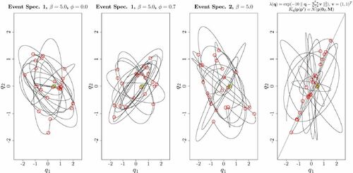
The rightmost panel of Figure 2 is included as an illustration of the flexibility afforded by GRHMCs as defined in Section 3.1. An event-rate favoring events occurring when the q-coordinate is close to (somewhere on) the subspace defined by ${\mathit{q}}_1={\mathit{q}}_2$ is considered. This is an example of a process where (unlike RHMC) the embedded discrete time process obtained by considering only the configuration at events is clearly off target, whereas the continuous time GRHMC process still has the desired stationary distribution. Such processes may be an avenue for obtaining between events dynamics amounting to (an integer multiple) of approximately half orbits. However, the selection of event-favoring subspaces for general non-Gaussian target distributions requires further research. From now on, only event specifications 1, $\varphi =0$ and 2 are considered.

3.5.1 Moment Estimation and “Super-convergence”

To gain some initial insight into the behavior of moment estimation based on NGRHMC processes, 10,000 trajectories of were generated for 4 zero mean, unit variance univariate targets $\pi ({\mathit{q}}_1)$. Each trajectory was of (time) length $T=1000\frac{\pi }{2}$ preceded by an equal length of warmup. Event specification 1, $\varphi =0$, was used in all cases, and experiments were repeated for different values of the inter-event mean time β (see Table 1). Further, several different sampling strategies were applied to all produced trajectories. Root mean squared errors (RMSEs) of the $E({\mathit{q}}_1)$-estimates are presented in Figure 3.

Fig. 3 RMSE of estimates of $E({\mathit{q}}_1)$ from NGRHMC processes using event specification 1 for different values of the mean inter-event time parameter β. The panels correspond to the different univariate target distributions $\pi ({\mathit{q}}_1)$, which all have zero mean and unit variance. Unit mass matrix M = 1 was used. The estimates of the mean are based on trajectories of length $T=1000\frac{\pi }{2}$, and the RMSE estimates are based on 10,000 independent replica for each value of β. Black circles correspond continuous sampling (7), red ×-s to 1000 equally spaced samples, blue squares to 500 equally spaced samples and green triangles to samples recorded at events only. The horizontal lines give the RMSE of 1000 iid samples. The results are obtained using the numerical methods described in Section 4.1 with $to{l}_a=to{l}_r=0.001$.

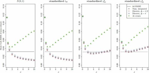
For the standard Gaussian distribution, exactly iid samples obtains when choosing trajectories of (time) length $\pi /2$ in the hypothetical HMC method (with exact dynamics, see Section 2.2). Thus, the (time) lengths of generated Hamiltonian flow (and thus essentially the computational cost) of NGRHMC and for 1000 iid-samples-producing hypothetical HMC transitions are the same. As a reference to the NGRHMC results, the RMSEs based on 1000 iid samples are indicated as horizontal lines in the plots. For the non-Gaussian targets, the cost of obtaining RMSEs corresponding to 1000 iid samples using HMC are likely somewhat higher, and thus the benchmarks are likely somewhat favoring HMC in a computational cost perspective in these cases.

In all cases, low values of β (frequent events) result in poor results, as the continuous time process approaches the Langevin limit (12). The most striking feature of the plot is that for continuous (black circles) or high frequency sampling (red ×) of the trajectories, RMSEs for the symmetric targets (N(0, 1), standardized t₂₀) decreases monotonically in β, and for the highest $\beta =10.0$ considered is only around 35% of the benchmark in the N(0, 1) case. In the univariate Gaussian target case, this behavior obtains as the between-event Hamiltonian dynamics, ${\mathit{q}}_1(t)$, averaged over time, that is, $\frac{1}{t}{\int }_0^t{\mathit{q}}_1(s)ds$, converges to the mean of the target as $t\to \infty$, regardless of the initial configuration $\mathit{z}(0)$ (see below and Appendix B, supplementary materials). Thus, in the Gaussian case, momentum refreshes are not necessary for unbiased estimation of $E({\mathit{q}}_1)$. It appears this is also the case for the standardized t₂₀-distribution, but this has not been proved formally so far.

For the nonsymmetric targets, standardized ${\chi }_{50}^2$ and standardized ${\chi }_{30}^2$, such monotonous behavior is not seen as momentum refreshes are certainly necessary to obtain high quality estimates. Too infrequent refreshes (i.e., high β) result in higher variance from exploring too few energy level sets. For intermediate values of β, the continuous- or high frequency sampling estimates are still better than or on par with the iid benchmark, where the edge is lost toward more skewness in the target distribution.

As mentioned in Section 2.3, the continuous time trajectories can either be sampled at discrete times (6) or continuously (in practice integrated numerically within the ODE solver, see below for details) over time (7), where the former may be thought of as a crude quadrature approximation to the latter. From Figure 3, it is evident that there is little difference in the high frequency ($\Delta =\pi /2$) discrete time sampling and continuous sampling. The efficiency deteriorates somewhat with more infrequent ($\Delta =\pi$) discrete sampling (blue $\square$). As will be clear in the next section, continuous estimates (7) require minimal additional numerical effort, and it seems advisable always to use these for moment calculations, whereas rather frequent discrete samples should be used for other tasks.

The green triangles represent results obtained when sampling the process only at event times using the same amount of Hamiltonian trajectory. It is seen that this practice, which does not exploit the “between-events” trajectories, generally lead to inferior results. The exception is in the random walk-like domain, where frequent events (and thus sampling) occur, but in this case the underlying process only slowly explores the target distribution.

3.6 Choosing Event Intensities

The time average property under the univariate Gaussian, illustrated in the left panel of Figure 3 generalizes to multivariate Gaussian targets $\pi (\mathit{q})=\mathcal{N}(\mathit{q}|\mu ,\Sigma )$ as well. Namely, it can be shown (see Appendix B, supplementary materials) that the between-events dynamics $\mathit{q}(\tau )$ admit unbiased estimation of μ without momentum refreshes, that is,(13) $$\frac{1}{T}{\int }_0^T\mathit{Cq}(\tau )d\tau \underset{T\to \infty }{\to }\mathit{C}\mu ,\mathit{C}\in {\mathbb{R}}^{p\times d},$$(13) regardless of the initial configuration $\mathit{z}(0)$.

Of course, the Gaussian case is not particularly interesting per se. However, one would presume that for near Gaussian target distributions (which is frequently the case in Bayesian analysis applications due to Bernstein-Von Mises effects), the left-hand side (13) would have only a small variation in $\mathit{z}(0)$ for large T. Hence, such situations would benefit from quite low event intensities/long durations between events and would allow for very small Monte Carlo variations in moment estimates akin to those shown in the two leftmost panels of Figure 3 even in high-dimensional applications.

Still, the fast convergence results above are restricted to certain moments of certain target distributions. It is instructive (and sobering) to look at the estimation of the second order moment of a univariate standard Gaussian target distribution (with $\mathit{M}=1$). In this case,$$\frac{1}{T}{\int }_0^T{\mathit{q}}_1^2(\tau )d\tau \underset{T\to \infty }{\to }\frac{1}{2}\left({\mathit{q}}_1^2(0)+{\mathit{p}}_1^2(0)\right),$$that is, the dependence on the initial configuration $\mathit{z}(0)$ does not vanish as the time between events grows, and the second order moment cannot be estimated reliably without momentum refreshes.

For a fixed budget of Hamiltonian trajectories, a non-Gaussian target and/or a nonlinear moment, say $E(g(\mathit{q}))$, and the event rate tradeoff will have at the endpoints:

• For “large β,” variation in the GRHMC moment estimate is mainly due to variation between energy level sets, that is, the variance of $\underset{T\to \infty }{\lim }{\int }_0^{T}g(\mathit{q}(t))dt$ as a function of the initial configuration $\mathit{z}(0)$.

• For “small β,” variation in the GRHMC moment estimate comes mainly from that the underlying process ${\mathcal{Z}}_t$ reverts to a random walk-like behavior (Langevin-dynamics for constant event rate).

The location of the optimum between these extremes (see, e.g., the two right-most panels in Figure 3) inherently depends both on the target distribution and the collection of moments, say $E(g_1(\mathit{q})),\dots ,E(g_m(\mathit{q}))$, one is interested in. More automatic choices of event rate specifications will be explored in the numerical experiments discussed below.

4 Numerical Implementation

The proposed methodology relies on quite accurate simulation of the Hamiltonian trajectories and associated functionals of the type (7). This section summarizes numerical implementation of these quantities based on Runge-Kutta-Nystöm (RKN) methods (see, e.g., Hairer, Nørsett, and Wanner 1993, chap. II.14). The reader is referred to Hairer, Nørsett, and Wanner (1993) for more background on general purpose ODE solvers.

In what follows, τ is used as the time index of the between-events Hamiltonian dynamics (as opposed to PDMP process time $t)$, and it is convention that τ is reset to zero immediately after each event. RKN methods are particularly well suited for time-homogenous second order ODE systems on the form(14) $$\stackrel{..}{\mathit{y}}(\tau )=\mathit{F}(\mathit{y}(\tau )),\mathit{y}\in {\mathbb{R}}^n,\mathit{F}:{\mathbb{R}}^n\mapsto {\mathbb{R}}^n,$$(14) subject to the initial conditions $\mathit{y}(0)={\mathit{y}}_0$, $\stackrel{.}{\mathit{y}}(0)={\mathit{z}}_0$. Notice that when F does not depend on $\stackrel{.}{\mathit{y}}(\tau )$, RKN methods are substantially more efficient than applying conventional Runge Kutta methods to an equivalent coupled system of 2n first order equations, say $\stackrel{.}{\mathit{y}}(\tau )=\mathit{w}(\tau ),\stackrel{.}{\mathit{w}}(\tau )=\mathit{F}(\mathit{y}(\tau ))$.

A wide range of numerical methods have been developed specifically for the dynamics of Hamiltonian systems (see, e.g., Sanz-Serna and Calvo 1994; Leimkuhler and Reich 2004). Such methods typically conserve the symplectic- and time-reversible properties of the true dynamics, and hence provide reliable long-term simulations over many (quasi-)orbits. However, for shorter time spans, typically on the order of up to a few (quasi-)orbits, such symplectic methods have no edge over conventional methods for second order ODEs (see, e.g., Sanz-Serna and Calvo 1994, sec. 9.3).

4.1 Numerical Solution of Dynamics and Functionals

In the numerical implementation used in the present work, the between-events Hamiltonian dynamics are reformulated in terms of the second order ODE(15) $$\stackrel{..}{\mathit{q}}(\tau )={\mathit{M}}^{-1}{\nabla }_{\mathit{q}}\hspace{0.17em}\text{log}\hspace{0.17em}(\mathit{q}(\tau )),$$(15) which is to be solved for $(\mathit{q}(\tau ),\stackrel{.}{\mathit{q}}(\tau ))$. The dynamics of (15) are equivalent to the dynamics of (2) when the initial conditions $(\mathit{q}(0),\stackrel{.}{\mathit{q}}(0)={\mathit{M}}^{-1}\mathit{p}(0))$ are applied, and the momentum variable for any τ is recovered via $\mathit{p}(\tau )=\mathit{M}\stackrel{.}{\mathit{q}}(\tau )$.

Further, recall that the proposed methodology relies critically on the ability to calculate between-events Hamiltonian dynamics functionals on the form(16) $${\mathit{r}}_k(\tau )={\int }_0^{\tau }{\mathit{M}}_k(\mathit{q}(s))ds,k=1,\dots ,p,$$(16) for a suitably chosen monitoring function $\mathit{M}:{\mathbb{R}}^d\to {\mathbb{R}}^p$, for example, for integrated event intensities Λ (4) and continuous sampling (7). To this end, first observe that $\mathit{r}(\tau )=\stackrel{.}{\mathit{R}}(\tau )$ whenever $\stackrel{..}{\mathit{R}}(\tau )=\mathit{M}(\mathit{q}(\tau )),$ with initial conditions $\mathit{R}(0)={\mathbf{0}}_p,\stackrel{.}{\mathit{R}}(0)={\mathbf{0}}_p$. Hence, by augmenting (15) with the monitoring function, that is,(17) $$\left[\begin{array}{c}\stackrel{..}{\mathit{q}}(\tau )\\ \stackrel{..}{\mathit{R}}(\tau )\end{array}\right]=\left[\begin{array}{c}{\mathit{M}}^{-1}{\nabla }_{\mathit{q}}\hspace{0.17em}\text{log}\hspace{0.17em}(\mathit{q}(\tau ))\\ \mathit{M}(\mathit{q}(\tau ))\end{array}\right],$$(17) a system on the form (14) is obtained. When solved numerically, (17) produces solutions both for the dynamics (2 or 15) and the dynamics functional (16). Implemented in this manner, the adaptive step size methodology (discussed in Appendix C) controls both the numerical error in the Hamiltonian dynamics and the functionals concurrently (in contrast to Nishimura and Dunson (2020) where integrator step sizes are kept fixed and intermediate integrator steps are included in averages based on an accept/reject mechanism).

In this work, the sixth order explicit embedded pair RKN method RKN6(4)6FD of (Dormand and Prince 1987, Table 2) was used to solve (17). Each step of RKN6(4)6FD requires five evaluations of the right-hand side of (17), but possesses improved stability properties relative to for example, the leapfrog method, hence, allowing for the use of larger step-sizes. Since the solution to $\mathit{R}(\tau )$ is not required per se, trivial modifications of the mentioned RKN method were done so that it solves only for $\mathit{s}(\tau )=(\mathit{q}(\tau ),\stackrel{.}{\mathit{q}}(\tau ),\mathit{r}(\tau ))$. Further details, and a full algorithm may be found in Section C in the Appendix, supplementary materials. It is also worth noticing that simpler, but less efficient variants of the above algorithm may be written in high level languages with access to off-the-shelf ODE solvers. Section G in the Appendix, supplementary materials gives an example written in R.

Table 2 Results for the “smile”-shaped target distribution (22,23).

γ	sampling		${\mathit{q}}_1$		$\underset{k\in \{2,11\}}{\min }\text{ESS}({\mathit{q}}_k)$		$\underset{k\in \{2,11\}}{\max }\text{ESS}({\mathit{q}}_k)$		$E({\mathit{q}}_1)$	$E({\mathit{q}}_2)$	CPU time
			ESS	$\frac{\text{ESS}}{\text{CPU}\mathrm{}\text{time}}$	ESS	$\frac{\text{ESS}}{\text{CPU}\mathrm{}\text{time}}$	ESS	$\frac{\text{ESS}}{\text{CPU}\mathrm{}\text{time}}$	(exact $=0$)	(exact $=1$)	(s)
rstan ($\max \widehat{R}=1.247$)
			19	10	29	15	32	17	–0.15	1.04	1.9
pdphmc, event specification 1, $\varphi =0$ (γ = 2: $\max \widehat{R}=1.006$, γ = 10: $\max \widehat{R}=1.015$)
2	D		1323	779	1065	627	1215	716	–0.02	1.03	1.7
2	C		1319	777	1115	657	1150	678	–0.02	1.02
10	D		2213	1304	608	358	634	374	0.01	1.00	1.7
10	C		2233	1316	613	361	630	371	0.01	1.01
pdphmc, event specification 2 (γ = 2: $\max \widehat{R}=1.007$, γ = 10: $\max \widehat{R}=1.009$)
2		D	1094	645	1130	666	1183	697	–0.02	0.98	1.7
2		C	1094	645	1153	679	1184	698	–0.02	0.97
10		D	2276	1341	920	542	967	570	0.01	1.03	1.7
10		C	2303	1357	927	546	948	559	0.01	1.03

NOTE: The results are based on 10 independent replica, and ESSes and ESSes per computing time are from the combined results over these replica. For rstan, each replica consists of the 10,000 transitions, with the former 5000 discarded as warmup. For pdphmc, ISG-type mass matrix, trajectories of length T = 25,000 divided evenly between warmup and sampling, and 1000 discrete samples were used. The presented CPU times are the total time spent by all chains/trajectories during the post warmup period. For each configuration of pdphmc, results from both discrete sampling (D) and continuous sampling (C) are presented.

4.2 Do Numerical Errors Influence Results?

To assess how the application of (un-corrected) RKN numerical integrators for the Hamiltonian dynamics influences overall Monte Carlo estimation, a small simulation experiment was performed. Specifically, a $N({\mathbf{0}}_2,\Sigma )$ target distribution with(18) $$\Sigma =\left[\begin{array}{cc}1& 2\\ 2& 8\end{array}\right],\mathit{M}={\mathit{I}}_2,\lambda =\frac{1}{10}\text{and}\mathrm{}Q(\mathit{p}|{\mathit{z}}^{\prime })=\mathcal{N}(\mathit{p}|{\mathbf{0}}_2,\mathit{M}),$$(18) was used. Due to the Gaussian nature of the target distribution, the Hamiltonian dynamics are available in closed form, and hence, allow the comparison with the numerically integrated counterparts. RHMC trajectories based both on exact and numerically integrated dynamics were used to estimate the mean and raw second order moments of the target using continuous sampling. The same initial configuration $\mathcal{Z}(0)$ and the same random numbers were used so that errors in the estimators based on numerical integration are due only to RKN integration. Figure 4 shows the RMSEs between estimates from numerically integrated- and exact RHMC trajectory for different values of T and the absolute (relative) RKN integrator error tolerance tol_a (tol_r) (see Appendix C, supplementary materials for details). All results are based on independent 50 replications. Also indicated in the plots as horizontal lines are the RMSEs associated with estimating the said moments (across multiple independent trajectories) based on RHMC with exact dynamics.

Fig. 4 Numerical errors incurred by RKN integration on the estimation the first and second order moments of a bivariate Gaussian target distribution. The numerical errors are relative to a NGRHMC trajectory using the same random numbers but with exact Hamiltonian dynamics. Both exact and numerically integrated results are based on continuous sampling. The horizontal axis gives the error tolerances (in all cases with $to{l}_a=to{l}_r$) applied in the numerical integrator, and both horizontal and vertical axis are logarithmic. Dotted lines indicate the root mean squared errors associated with estimating the indicated moments across many exact NGRHMC trajectories of different length T.

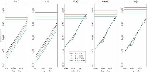
From Figure 4, it is seen that except for very large values of $to{l}_a=to{l}_r$, the numerical errors are very small relative to the exact estimator RMSEs. From the plots, absolute and relative error tolerances of around 0.001 appear to be more than sufficient for this case. Interestingly, it is seen that there is no apparent buildup of numerical errors in the longer trajectories, suggesting that the incurred errors are not systematically accumulating and biasing the estimation in any direction. Of course, this limited experiment does not rule out such biasing behavior in general. However, the overall the finding here indicate that quite lax error tolerances are sufficient to make the numerical errors be negligible relative to overall Monte Carlo variation.

More formal characterizations of the incurred biases is another avenue for further work. Such approaches could involve either theoretically bounding the biases incurred in Wasserstein distance, for example, based on the techniques of Rudolf and Schweizer (2018). More numerically oriented approaches using Multilevel Monte Carlo methods (see, e.g., Giles 2015), based on multiple trajectories with different error tolerances but the same random number seed would be another alternative.

4.3 Automatic Selection of Tuning parameters

A key aim of developing NGRHMC processes is to enable the implementation of an easy to use and general-purpose code. For this purpose, automatic selection of tuning parameters is important. This Section describes the routines for tuning the mass matrix M and scaling the event intensity used in the computations described shortly.

4.3.1 Tuning of Mass Matrix

In the present work, only a diagonal mass matrix $\mathit{M}=\text{diag}(m_1,\dots ,m_d)$ is considered. Two approaches for choosing each of $m_1,\dots ,m_d$ are considered, both exploiting the ability to numerically calculate temporal averages by augmenting the monitoring function $\mathit{M}$.

In the former approach which will be referred to as VARI (variance, integrated), $m_i^{-1}$ is simply set equal to the temporal average estimate of $\text{var}({\mathit{q}}_i)$, that is,$${\int }_0^{t^{*}}{\mathcal{Q}}_i^2(s)ds-{\left[{\int }_0^{t^{*}}{\mathcal{Q}}_i(s)ds\right]}^2,$$at every event time $t^{*}$ during the warmup period.

In cases where the marginal variances are less informative with respect to the local scaling of the target distribution, for example, in the presence of strong nonlinearities or multimodality, a second approach referred to as ISG (integrated squared gradients) may also pursued. Here overarching idea for choosing each of $m_1,\dots ,m_d$ is to make the square of each element of the right-hand side of (15), averaged over each integrator step, in expectation over all integrator steps, to be equal to 1. This approach is mainly motivated out of numerical efficiency considerations, where regions of the target distribution requiring many steps (with short step sizes due to strong forces ${\nabla }_{\mathit{q}}\hspace{0.17em}\text{log}\hspace{0.17em}\tilde{\pi }(\mathit{q})$) are disproportionally weighted when choosing the mass matrix.

More explicitly, let the jth integrator step (during the warmup period) be originating at time τ_j and have time step size ${\epsilon }_j$. Then the mass matrix diagonal m_i is taken to be an exponential moving average (over j) of$$\frac{1}{{\epsilon }_j}{\int }_{{\tau }_j}^{{\tau }_j+{\epsilon }_j}{\left[{\nabla }_{\mathit{q}}\hspace{0.17em}\text{log}\hspace{0.17em}\tilde{\pi }(\mathit{q}(s))\right]}_i^{2}ds.$$

Notice that the integrated squared gradients are available at negligible additional cost by augmenting $\mathit{M}$ in the ODE system (17) with moment functions ${\left[{\nabla }_{\mathit{q}}\hspace{0.17em}\text{log}\hspace{0.17em}\tilde{\pi }(\mathit{q})\right]}_i^2,i=1,\dots ,d$. Further notice that for a $N(\mu ,{\mathit{P}}^{-1})$ target distribution, where $E_{\pi }(\left[{\nabla }_{\mathit{q}}\hspace{0.17em}\text{log}\hspace{0.17em}\tilde{\pi }(\mathit{q})\right]{\left[{\nabla }_{\mathit{q}}\hspace{0.17em}\text{log}\hspace{0.17em}\tilde{\pi }(\mathit{q})\right]}^T)=\mathit{P}$, this approach may (modulus variability in integrator step size) be seen as a way to directly estimate the precision matrix diagonal elements.

4.3.2 Tuning of Event Rates

The methodology for tuning the event rates relies of the following representation of a general event rate λ:$$\lambda (\mathit{q},\mathit{p})=\frac{1}{\gamma \beta }\overline{\lambda }(\mathit{q},\mathit{p}),\gamma >0,\beta >0,$$where $\overline{\lambda }$ is a “base line” event rate (e.g., $\overline{\lambda }=1$ for event specification 1 and 2, and $\overline{\lambda }=\sqrt{{\mathit{p}}^T{\mathit{M}}^{-1}\mathit{p}}$ for event specification 2). Here γ is a user-given scale factor, say in the range 1–20, chosen in the higher range if one expects good performance with infrequent moment refreshes (see Section 3.6). Finally, β is tuned automatically to reflect each particular target distribution and event specification.

Suppose $\iota (\mathit{z})$ is the distribution the state immediately after events (which is equal to $\rho (\mathit{z})$ for RHMC but may also differ substantially relative to $\rho (\mathit{z})$ as seen in the rightmost panel of Figure 2). The objective of the automatic event rate tuning is given by(19) $$\begin{array}{c}\underset{\mathit{z}(0)\sim \iota (\mathit{z})}{E}{\beta }^{-1}\Upsilon (\mathit{z}(0))=1,\mathrm{}\text{where}\\ \hspace{1em}\Upsilon (\mathit{z}(0))={\int }_0^{\omega (\mathit{z}(0))}\overline{\lambda }(\mathit{q}(\tau ),\mathit{p}(\tau ))d\tau ,\end{array}$$(19) and where ω is the “U-turn” time (Hoffman and Gelman 2014)$$\omega (\mathit{z}(0))=\inf \left\{\tau >0:{(\mathit{q}(\tau )-\mathit{q}(0))}^T\mathit{p}(\tau )<0\right\},$$ of the dynamics (2) initialized at $\mathit{z}(0)$ (See also Wu, Stoehr, and Robert 2018, for a similar development). The rationale behind (19) is that (for γ = 1) the expected integrated event rate Λ (see Equation 4(4) $$\Lambda (v;\mathcal{Z}(t))=u,\text{where}\mathrm{}\Lambda (v;\mathit{z})={\int }_0^v\lambda ({\Xi }_s(\mathcal{Z}(t)))ds.$$(4) ) evaluated at corresponding U-turn time is equal to E(u).

In the present implementation, $\Upsilon (\mathit{z}(0))$ is computed for each event during warmup with $\mathit{z}(0)$ being the state immediately after the events. Subsequently, ${\beta }^{-1}$ is updated (also during the warmup period only) at each event according to an exponential moving average over the already computed $\Upsilon$s. The exponential moving average is used as the older realizations of $\Upsilon$ are typically recorded with a different mass matrix encountered earlier in the mass matrix adaptation process. Computing $\Upsilon (\mathit{z}(0))$ for each event incurs only modest additional costs, since $\Upsilon$ is a scalar integrated quantity computed over Hamiltonian dynamics that are integrated numerically anyway. However, if the next event occurs before the U-turn time ω, further integration steps are performed until ω is reached. The additional (post-event) Hamiltonian dynamics used to locate ω are subsequently discarded.

5 Numerical Experiments

This section considers numerical experiments and benchmarking of the proposed method against the NUTS-HMC implementation in Stan (rstan version 2.21.2). Like Stan, the proposed methodology has been implemented as an R package (pdphmc) with main computational tasks done in C++, and relies, like rstan, on the Stan Math Library (Carpenter et al. 2017) for automatic differentiation and probability- and linear-algebra computations.

All computations in this section were carried out on a 2020 Macbook pro with a 2.6 GHz Intel Core i7 processor, under R version 4.0.3. In line with the findings in Section 4.2, the default integrator tolerances $to{l}_a=to{l}_r=0.001$ are used for pdphmc unless otherwise noted. The package pdphmc, and code and data for reproducing the reported results is available at https://github.com/torekleppe/PDPHMCpaperCode.

In order to compare the performance of the methods, their effective sample size (ESS) (Geyer 1992) per computing time (see, e.g., Girolami and Calderhead 2011) is taken as the main statistic. Consider a sample dependent of dependent random variables ${\eta }_i,i=1,\dots ,N$, each having the same marginal distribution. The ESS gives the number of hypothetical iid samples (with distribution equal to that of η₁) required to obtain a mean estimator with the same variance as $N^{-1}{\sum }_{i=1}^N{\eta }_i$. An ESS-based approach is taken also here, but in order to obtain ESSes for moments estimated by for integrated quantities (7), the following approach was taken: For a given number of samples, say N, rewrite the left-hand side of (7) as(20) $$\begin{array}{c}\frac{1}{T}{\int }_0^{T}g(\mathcal{Z}(t))dt=\frac{1}{N}\sum _{i=1}^N{\eta }_i,\text{where}\\ \hspace{1em}{\eta }_i={\Delta }^{-1}{\int }_{(i-1)\Delta }^{i\Delta }g(\mathcal{Z}(t))dt,\Delta =\frac{T}{N}.\end{array}$$(20)

Let ${\widehat{\text{ESS}}}_i({\eta }_i)$ denote an estimator of the ESS of dependent sample η_i. Then(21) $$\frac{{\widehat{\text{var}}}_i(g(\mathcal{Z}(\Delta i)))}{{\widehat{\text{var}}}_i({\eta }_i)}{\widehat{\text{ESS}}}_i({\eta }_i)$$(21) is taken to be an estimator of ESS represented by moment estimator $T^{-1}{\int }_0^{T}g(\mathcal{Z}(t))dt$, expressed in terms of iid samples of $g(\mathit{q})$. Equation (21)(21) $$\frac{{\widehat{\text{var}}}_i(g(\mathcal{Z}(\Delta i)))}{{\widehat{\text{var}}}_i({\eta }_i)}{\widehat{\text{ESS}}}_i({\eta }_i)$$(21) takes into account both that ${\widehat{\text{var}}}_i({\eta }_i)$ tends to be smaller than ${\widehat{\text{var}}}_i(g(\mathcal{Z}(\Delta i)))$ due to the temporal averaging in (20), but on the other hand η_i tends to exhibit a stronger autocorrelation than discrete time samples $g(\mathcal{Z}(\Delta i))$. Throughout this text, the ESS estimation procedure in rstan (see R-function rstan::monitor(), output “n_eff”) was used for estimating ESS from samples. In addition, the largest (over sampled quantities) Gelman-Rubin $\widehat{R}$ statistics ($\max \widehat{R}$) (Gelman et al. 2014) were computed using the same function. For pdphmc, the reported $\max \widehat{R}$ are computed for the discretely sampled processes.

Comparing the performance of different MCMC methods is intrinsically hard. Care has been taken so that all code is written in the same language and compiled with the same compiler on the same computer and so on. Still, in the present context one must also consider that rstan is based on an “exact” MCMC scheme whereas pdphmc will in general be subject to (arbitrarily small, at the cost of more computing,) biases stemming from the use of uncorrected numerical integration. On the other hand, as demonstrated for example, in Figure 1, chains of finite length generated by rstan may fail to reflect the target distribution in cases where no visible bias is exhibited by pdphmc due to the adaptive nature of the applied integrators. The relative weighting of these features naturally depends on the application at hand, and therefore preclude strong conclusions regarding the relative performance of the methods.

In what follows, three numerical experiments are presented. A further experiment, based on a crossed random effects model for the Salamander data is described in Section D of the Appendix, supplementary materials. For the Salamander data, pdphmc is found to be on par or somewhat more efficient than rstan.

5.1 Funnel Distribution

The Funnel distribution ${\mathit{q}}_1\sim N(0,1),{\mathit{q}}_2|{\mathit{q}}_1\sim N(0,\hspace{0.17em}\text{exp}\hspace{0.17em}(3{\mathit{q}}_1))$ (funnel distributions may be traced back to Neal 2003), constituting the first numerical example, has already been encountered in Section 2.2 and Figure 1. This very simple example may be considered as a “model problem” displaying similar behavior as for targets associated with Bayesian hierarchical models (where q₁ plays the role of latent field log-scale parameter, and q₂ plays the role of the latent field it self).

For both rstan and pdphmc, 10 independent chains/trajecto- ries were run with identity mass matrices. For rstan, each of these chains had 10,000 transitions with 5000 discarded as warmup. The number of warmup iterations is larger than the default 1000 to allow for best possible integrator step size adaptation. The remaining tuning parameters of rstan are the default. Note that rstan outputs a substantial number of warnings related to diverged transitions for all values of δ.

For pdphmc, the trajectories were of length T = 100,000, sampled discretely N = 10,000 times and with the former half of samples discarded as warmup. For such high sampling frequency, continuous samples yield similar results as the discrete samples, and are not discussed further here. A constant event rate $\lambda ={\beta }^{-1}$ was applied, and β was adapted with scale factor γ = 2 using the methodology described in Section 4.3.2. The adaptive selection resulted in values of β between 2.1 and 4.7 across the 10 trajectories, which again translates to between 0.21 and 0.48 discrete time samples per (between-events) Hamiltonian trajectory.

It has already been confirmed visually from Figure 1 that the output of rstan does not fully explore the target distribution as fixed time step size integration is broadly speaking unsuitable for this problem. Consequently, ESSes for rstan are not presented. pdphmc produces around 800 effective samples per second for the log-scale parameter ${\mathit{q}}_1$. This is close to double what one obtains by calculating time-weighted ESS for the (still defective) $\delta =0.999$ rstan chains, indicating the proposed methodology is highly competitive for difficult problems (as even smaller fixed time steps would be required to obtain proper convergence). Further, the default integrator tolerances $to{l}_a=to{l}_r=0.001$ lead to biases (relative to the theoretical process) that are not detectable from the right panel of Figure 1.

5.2 Smile-Shaped Distribution

To further explore the performance of pdphmc applied to a highly nonlinear target distributions; the “smile”-shaped distribution(22) $${\mathit{q}}_k|{\mathit{q}}_1\sim N({\mathit{q}}_1^2,{0.5}^2),k=2,\dots ,11,$$(22) (23) $${\mathit{q}}_1\sim N(0,1)$$(23) is considered. The results for various settings of pdphmc and rstan are given in Table 2. From the Table, it is seen that rstan has substantial convergence problems with the largest Gelman-Rubin $\widehat{R}>1.05$, whereas the various settings of pdphmc reliably explores the target. Choosing longer trajectories (γ = 10) results in higher sampling efficiency for the marginally standard Gaussian ${\mathit{q}}_1$, whereas for the non-Gaussian components ${\mathit{q}}_{2:11}$, shorter trajectories are more efficient. Comparing the event specifications 1 and 2, it is seen that none of them produces uniformly better results.

5.3 Logistic Regression

The next example model is a basic logistic regression model(24) $${\mathit{y}}_i|\mathit{\beta }\sim \text{Beroulli}({\mathit{p}}_i),\text{logit}({\mathit{p}}_i)={\mathit{x}}_{i,·}^T\mathit{\beta },i=1,\dots ,n,$$(24) (25) $$\mathit{\beta }\sim N({\mathbf{0}}_p,100{\mathit{I}}_p)$$(25) applied to the German credit data (see, e.g., Michie, Spiegelhalter, and Taylor 1994) which has n = 1000 examples and p = 25 covariates (including a constant term). This example is included to measure the performance relative to rstan on an “easy” target distribution (Chopin and Ridgway 2017).

Results for pdphmc and rstan are provided in Table 3. It is seen that rstan produces less variation in the ESSes across the different parameters than pdphmc, which presumably is related to the mass matrix adaptation. The discrete samples cases of pdphmc have a somewhat slower minimum ESS performance but on par or better median- and maximum ESS performance. For this target distribution, continuous samples for the first moment of $\mathit{\beta }|\mathit{y}$ substantially improves the performance of pdphmc relative to the corresponding discretely sampled counterparts in all cases.

Table 3 ESSes and time weighted ESSes for the logistic regression model (24,25) applied to the German credit data.

γ	Sampling	${\min }_j$ $\widehat{\text{ESS}}({\mathit{\beta }}_j)$		${\text{median}}_j$ $\widehat{\text{ESS}}({\mathit{\beta }}_j)$		${\max }_j$ $\widehat{\text{ESS}}({\mathit{\beta }}_j)$		CPU
		ESS	$\frac{\text{ESS}}{\text{CPU}\mathrm{}\text{time}}$	ESS	$\frac{\text{ESS}}{\text{CPU}\mathrm{}\text{time}}$	ESS	$\frac{\text{ESS}}{\text{CPU}\mathrm{}\text{time}}$	time
rstan ($\max \widehat{R}=1.003$)
		9676	2125	13450	2953	15812	3472	4.55
pdphmc, event specification 1 (γ = 5: $\max \widehat{R}=1.011$, γ = 20: $\max \widehat{R}=1.020$)
5	D	11350	1425	23114	2903	40000	5023	7.96
5	C	18220	2288	32967	4140	71079	8926
20	D	11853	1490	29752	3740	40000	5028	7.96
20	C	20423	2567	36019	4528	69623	8752
pdphmc, event specification 2 ($\gamma =5$: $\max \widehat{R}=1.007$, γ = 20: $\max \widehat{R}=1.027$)
5	D	11281	1362	23185	2799	40000	4829	8.28
5	C	18317	2211	30771	3715	66928	8080
20	D	12780	1565	32653	3999	40000	4899	8.16
20	C	20902	2560	43303	5304	70584	8645

NOTE: All figures are based on 10 independent chains/trajectories. For rstan, the default 1000 warmup transitions followed by 1000 sampling transitions were used. For pdphmc, a VARI mass matrix, T = 5000 divided evenly between warmup and sampling and 1000 discrete samples per trajectory were used.

6 Dynamic Inverted Wishart Model for Realized Covariances

6.1 Model and Data

As a large scale illustrative application of NGRHMC, the dynamic inverted Wishart model for realized covariance matrices (Golosnoy, Gribisch, and Liesenfeld 2012) of Grothe, Kleppe, and Liesenfeld (2019) is considered. Under this model, a time series of SPD covariance matrices ${\mathit{Y}}_k\in {\mathbb{R}}^{G\times G},k=1,\dots ,n$ are modeled independently inverted Wishart distributed conditionally on a latent time-varying SPD scale matrix ${\mathit{\Sigma }}_k$ and a degree of freedom parameter $\nu >G+1$, that is,(26) $${\mathit{Y}}_k|{\mathit{\Sigma }}_k,\nu \sim \text{inv}-\text{Wishart}(\nu ,{\mathit{\Sigma }}_k)$$(26)

so that $E({\mathit{Y}}_k|{\mathit{\Sigma }}_k,\nu )={(\nu -G-1)}^{-1}{\mathit{\Sigma }}_k$. The time-varying scale matrix is in turn specified in terms of(27) $${\mathit{\Sigma }}_k=\mathit{H}[\text{diag}(\hspace{0.17em}\text{exp}\hspace{0.17em}({\mathit{x}}_{1,k}),\dots ,\hspace{0.17em}\text{exp}\hspace{0.17em}({\mathit{x}}_{G,k}))]{\mathit{H}}^T$$(27) where $\mathit{H}\in {\mathbb{R}}^{G\times G}$ is a lower triangular matrix with ${\mathit{H}}_{g,g}=1,g=1,\dots ,G$. The remaining (strictly lower triangular) elements ${\mathit{H}}_{i,j},j=1,\dots ,G-1,i=j+1,\dots ,G,$ are unrestricted parameters. Finally, the log-scale factors ${\mathit{x}}_{g,k}$ are a priori independent (over g) stationary Gaussian AR(1) processes(28) $$\begin{array}{c}{\mathit{x}}_{g,k}={\mathit{\mu }}_g+{\mathit{\delta }}_g({\mathit{x}}_{g,k-1}-{\mathit{\mu }}_g)+{\mathit{\sigma }}_g{\epsilon }_{g,k},{\epsilon }_{g,k}\sim \text{iid}\mathrm{}N(0,1),\\ \mathrm{\hspace{1em}}\mathrm{\hspace{1em}}k=2,\dots ,n,g=1,\dots ,G,\end{array}$$(28) (29) $${\mathit{x}}_{g,1}\sim N\left({\mathit{\mu }}_g,{\mathit{\sigma }}_g^2/(1-{\mathit{\delta }}_g^2)\right),g=1,\dots ,G,$$(29) where ${\mathit{\mu }}_g,{\mathit{\delta }}_g\in (-1,1),{\mathit{\sigma }}_g>0,g=1,\dots ,G$are parameters.

The joint distribution of parameters $\mathit{\theta }=(\mathit{\mu },\mathit{\delta },\mathit{\sigma },{\mathit{H}}_{2:G,1},\dots ,{\mathit{H}}_{G,G-1},\nu )$ and latent variables x is difficult to sample from, and in order to reduce “funnel” effects, the Laplace-based transport map reformulation of Osmundsen, Kleppe, and Liesenfeld (2021) (without Newton iterations) is used here. For every admissible $\mathit{\theta }$, a smooth bijective mapping, say $\mathit{x}={\gamma }_{\mathit{\theta }}(\mathit{z}),\mathit{z}\in {\mathbb{R}}^{Gn}$, is introduced so that $p(\mathit{z},\mathit{\theta }|{\mathit{Y}}_{1:n})\propto |{\nabla }_{\mathit{z}}\text{vec}({\gamma }_{\mathit{\theta }}(\mathit{z}))|{[p(\mathit{x},\mathit{\theta }|{\mathit{Y}}_{1:n})]}_{\mathit{x}={\gamma }_{\mathit{\theta }}(\mathit{z})}$ approximates $p(\mathit{\theta }|{\mathit{Y}}_{1:n})\mathcal{N}(\mathit{z}|{\mathbf{0}}_{Gn},{\mathit{I}}_{Gn})$. Subsequently, NGRHMC/HMC targeting $p(\mathit{z},\mathit{\theta }|{\mathit{Y}}_{1:n})$ are performed. The reader is referred Appendix E and Osmundsen, Kleppe, and Liesenfeld (2021) for more details on the construction of ${\gamma }_{\mathit{\theta }}$ and Appendix E, supplementary materials for further details such as priors.

The data considered are n = 2514 daily observations of realized covariance matrices for G = 5 stocks (American Express, Citigroup, General Electric, Home Depot, IBM) between January 1, 2000 and December 31, 2009. See Golosnoy, Gribisch, and Liesenfeld (2012) for details on how this dataset was constructed from high frequency financial data. For these values of n and G, the model involves Gn = 12570 latent variables and $3G+G(G-1)/2+1=26$ parameters.

6.2 Results

ESSes and time-weighted ESSes for the parameters, ${\mathit{z}}_{1:5,1}$ and ${\mathit{x}}_{1:5,1}$ are given in Table 4 for two variants of pdphmc and an rstan benchmark. It is seen that the discretely sampled (D) pdphmc uniformly provides faster sampling performance than rstan. The speedup is in particularly significant when taking all (A) computations into account as rstan uses more than 80% of the computing time in the warmup phase, whereas there is relatively little warmup overhead for pdphmc. For continuously sampled (C) pdphmc the picture is somewhat more mixed with numbers ranging from being on par with rstan ($\mathit{\delta }$, event specification 2) to being up to five times faster (H, both event specifications). Event specification 2 lead to better worst-case performance than event specification 1 in all cases other than for H. However, the differences are not very large which may be explained by the high dimensionality of the model, and that event specifications 1 and 2 are very similar in this case. Still this observation suggest that it may be possible to gain even more efficiency by developing better adaptive event rate specifications.

Table 4 Effective sample sizes and computing times for the dynamic inverted Wishart model (26,29).

		rstan	pdphmc, event spec. 1, $\gamma =10.0$ (10629, 25244) 1.032		pdphmc, event spec. 2, $\gamma =10.0$ (10189, 24960) 1.034
	CPU time (S,A)	(14605, 72127)
	$\max \widehat{R}$	1.003
	sampling		D	C	D	C
$\mathit{\mu }$	ESS (min, max)	(14304, 18487)	(12906, 28173)	(14467, 28370)	(14749, 38387)	(14224, 41821)
	ESS/S (min, max)	(0.98, 1.27)	(1.21, 2.65)	(1.36, 2.67)	(1.45, 3.77)	(1.40, 4.10)
	ESS/A (min, max)	(0.20, 0.26)	(0.51, 1.12)	(0.57, 1.12)	(0.59, 1.54)	(0.57, 1.68)
$\mathit{\sigma }$	ESS (min, max)	(14757, 20011)	(28447, 38922)	(35971, 42891)	(30227, 40000)	(34283, 44316)
	ESS/S (min, max)	(1.01, 1.37)	(2.68, 3.66)	(3.38, 4.04)	(2.97, 3.93)	(3.36, 4.35)
	ESS/A (min, max)	(0.20, 0.28)	(1.13, 1.54)	(1.42, 1.70)	(1.21, 1.60)	(1.37, 1.78)
$\mathit{\delta }$	ESS (min, max)	(13624, 16678)	(16145, 28401)	(18109, 31180)	(15749, 25582)	(9464, 29271)
	ESS/S (min, max)	(0.93, 1.14)	(1.52, 2.67)	(1.70, 2.93)	(1.55, 2.51)	(0.93, 2.87)
	ESS/A (min, max)	(0.19, 0.23)	(0.64, 1.13)	(0.72, 1.24)	(0.63, 1.02)	(0.38, 1.17)
H	ESS (min, max)	(12195, 22072)	(35292, 40000)	(46273, 69861)	(33089, 40000)	(43658, 70275)
	ESS/S (min, max)	(0.84, 1.51)	(3.32, 3.76)	(4.35, 6.57)	(3.25, 3.93)	(4.28, 6.90)
	ESS/A (min, max)	(0.17, 0.31)	(1.40, 1.58)	(1.83, 2.77)	(1.33, 1.60)	(1.75, 2.82)
ν	ESS	17797	40000	53388	40000	56313
	ESS/S	1.22	3.76	5.02	3.93	5.53
	ESS/A	0.25	1.58	2.11	1.60	2.26
${\mathit{z}}_{1,·}$	ESS (min, max)	(22130, 24317)	(30533, 40000)	(37065, 70920)	(40000, 40000)	(64787, 68952)
	ESS/S (min, max)	(1.52, 1.67)	(2.87, 3.76)	(3.49, 6.67)	(3.93, 3.93)	(6.36, 6.77)
	ESS/A (min, max)	(0.31, 0.34)	(1.21, 1.58)	(1.47, 2.81)	(1.60, 1.60)	(2.60, 2.76)
${\mathit{x}}_{1,·}$	ESS (min, max)	(22149, 24858)	(27525, 40000)	(33768, 70763)	(40000, 40000)	(63230, 68873)
	ESS/S (min, max)	(1.52, 1.70)	(2.59, 3.76)	(3.18, 6.66)	(3.93, 3.93)	(6.21, 6.76)
	ESS/A (min, max)	(0.31, 0.34)	(1.09, 1.58)	(1.34, 2.80)	(1.60, 1.60)	(2.53, 2.76)

NOTE: In all cases, the results are based on 10 independent chains/trajectories and reported computing times are the total computing times over these 10 replica. For rstan, default sampler parameters with 1000 warmup transitions followed by 1000 sampling transitions were used. For pdphmc, T = 5000 split evenly between warmup and sampling, 1000 samples and an VARI type diagonal mass matrix were applied. Both computing times for the sampling (S) period and for all (A) computations (warmup and sampling) are provided, and ESSes are weighted both for S and A.

Posterior means and standard deviations obtained both from rstan and discretely sampled pdphmc presented in Table 6 in the Appendix show no noteworthy deviations (see also Grothe, Kleppe, and Liesenfeld 2019, Table 5). To conclude, pdphmc is fast and reliable alternative to HMC that also scale well to high-dimensional settings.

7 Discussion

This article has introduced numerical generalized randomized HMC processes as a new, robust and potentially very efficient alternative to conventional MCMC methods. The presently proposed methodology holds promise to be substantially more trustworthy for complicated real-life problems. This improvement is related to two factors:

• The NGRHMC process is defined in continuous time and is time-irreversible. The present article is to the author’s knowledge the among the first attempts to leverage time-irreversible processes to produce general purpose and easy to use MCMC-like samplers that scale to high-dimensional problems. By now, there is substantial evidence (see, e.g., discussion on p. 387 of Fearnhead et al. 2018) that such irreversible processes are superior to conventional reversible alternatives.

• The proposed implementation of NGRHMC process leverages the mature, and widely used field of numerical integration of ordinary differential equations. Common practice for HMC is choosing a fixed step size low order symplectic method and hoping that regions where this step size is too large for numerical stability is not encountered during the simulation. The proposed methodology, on the other hand, relies on high quality adaptive integrators, which have no such stability problems.

Currently, efficient and robust MCMC computations has been a field dominated by tailor-making to specific applications and a large degree of craftsmanship. Effectively, the two above points reduces such MCMC computations into a more routine task of numerically integrating ordinary differential equations using adaptive/automatic methods.

There is scope for substantial further work on NGRHMC-processes beyond the initial developments given here. A, by no means complete, list of possible further research directions related to NGRHMC processes is given in Appendix F, supplementary materials.

Acknowledgments

The author wishes to express thanks to the Editor, Professor McCormick, an anonymous Associate Editor, and three anonymous reviewers who have contributed with many constructive comments which have sparked numerous improvements to the article.

Supplementary Materials

The supplementary material is a pdf-file containing: A: various detailed derivations, B: Temporal averages of the Hamiltonian dynamics for Gaussian targets, C: Details related to numerical implementation, D: additional numerical experiment: Salamander mating data, E: details of the inverted Wishart model, F: suggestions for further work, G: A simple R implementation.

References

- Abraham, M. J., Murtola, T., Schulz, R., Páll, S., Smith, J. C., Hess, B., and Lindahl, E. (2015), “GROMACS: High Performance Molecular Simulations Through Multi-Level Parallelism from Laptops to Supercomputers,” SoftwareX, 1–2, 19–25. DOI: 10.1016/j.softx.2015.06.001.
- Andersen, H. C. (1980), “Molecular Dynamics Simulations at Constant Pressure and/or Temperature,” The Journal of Chemical Physics, 72, 2384–2393. DOI: 10.1063/1.439486.
- Bierkens, J., Fearnhead, P., and Roberts, G. (2019), “The Zig-Zag Process and Super-Efficient Sampling for Bayesian Analysis of Big Data,” The Annals of Statistics, 47, 1288–1320. DOI: 10.1214/18-AOS1715.
- Bierkens, J., Grazzi, S., Kamatani, K., and Roberts, G. (2020), “The Boomerang Sampler,” arXiv:2006.13777.
- Bou-Rabee, N., and Eberle, A. (2020), “Couplings for Andersen Dynamics,” arXiv:2009.14239.
- Bou-Rabee, N., and Eberle, A. (2021), “Mixing Time Guarantees for Unadjusted Hamiltonian Monte Carlo,” arXiv:2105.00887.
- Bou-Rabee, N., and Sanz-Serna, J. M. (2017), “Randomized Hamiltonian Monte Carlo,” Annals of Applied Probability, 27, 2159–2194.
- Bou-Rabee, N., and Sanz-Serna, J. M. (2018), “Geometric Integrators and the Hamiltonian Monte Carlo Method,” Acta Numerica, 27, 113–206.
- Bou-Rabee, N., and Schuh, K. (2020), “Convergence of Unadjusted Hamiltonian Monte Carlo for Mean-Field Models,” arXiv:2009.08735.
- Bouchard-Côté, A., Vollmer, S. J., and Doucet, A. (2018), “The Bouncy Particle Sampler: A Nonreversible Rejection-Free Markov Chain Monte Carlo Method,” Journal of the American Statistical Association, 113, 855–867. DOI: 10.1080/01621459.2017.1294075.
- Cambanis, S., Huang, S., and Simons, G. (1981), “On the Theory of Elliptically Contoured Distributions,” Journal of Multivariate Analysis, 11, 368–385. DOI: 10.1016/0047-259X(81)90082-8.
- Cances, E., Legoll, F., and Stoltz, G. (2007), “Theoretical and Numerical Comparison of Some Sampling Methods for Molecular Dynamics,” ESAIM: Mathematical Modelling and Numerical Analysis, 41, 351–389. DOI: 10.1051/m2an:2007014.
- Carpenter, B., Gelman, A., Hoffman, M., Lee, D., Goodrich, B., Betancourt, M., Brubaker, M., Guo, J., Li, P., and Riddell, A. (2017), “Stan: A Probabilistic Programming Language,” Journal of Statistical Software, 76, 1–32. DOI: 10.18637/jss.v076.i01.
- Chen, Z., and Vempala, S. S. (2019), “Optimal Convergence Rate of Hamiltonian Monte Carlo for Strongly Logconcave Distributions,” in Approximation, Randomization, and Combinatorial Optimization. Algorithms and Techniques, APPROX/RANDOM 2019, September 20–22, 2019, Massachusetts Institute of Technology, Cambridge, MA, USA, Volume 145 of LIPIcs, eds. D. Achlioptas and L. A. Végh, pp. 64:1–64:12, Schloss Dagstuhl - Leibniz-Zentrum für Informatik.
- Cheng, X., Chatterji, N. S., Bartlett, P. L., and Jordan, M. I. (2018), “Underdamped Langevin mcmc: A Non-asymptotic Analysis,” in Proceedings of the 31st Conference On Learning Theory, Volume 75 of Proceedings of Machine Learning Research, eds. S. Bubeck, V. Perchet, and P. Rigollet, pp. 300–323. PMLR.
- Chopin, N., and Ridgway, J. (2017), “Leave Pima Indians Alone: Binary Regression as a Benchmark for Bayesian Computation,” Statistical Science, 32, 64–87. DOI: 10.1214/16-STS581.
- Cotter, S., House, T., and Pagani, F. (2020), “The NuZZ: Numerical ZigZag Sampling for General Models,” arXiv:2003.03636.
- Davis, M. H. A. (1984), “Piecewise-Deterministic Markov Processes: A General Class of Non-diffusion Stochastic Models,” Journal of the Royal Statistical Society, Series B, 46, 353–376. DOI: 10.1111/j.2517-6161.1984.tb01308.x.
- Davis, M. H. A. (1993), Markov Models and Optimization, London: Chapman & Hall.
- Deligiannidis, G., Paulin, D., Bouchard-Côté, A., and Doucet, A. (2018), “Randomized Hamiltonian Monte Carlo as Scaling Limit of the Bouncy Particle Sampler and Dimension-Free Convergence Rates,” arXiv:1808.04299.
- Dormand, J., and Prince, P. (1987), “Runge-Kutta-Nystrom Triples,” Computers & Mathematics with Applications, 13, 937–949.
- Fang, Y., Sanz-Serna, J. M., and Skeel, R. D. (2014), “Compressible Generalized Hybrid Monte Carlo,” The Journal of Chemical Physics, 140, 174108. DOI: 10.1063/1.4874000.
- Fearnhead, P., Bierkens, J., Pollock, M., and Roberts, G. O. (2018), “Piecewise Deterministic Markov Processes for Continuous-Time Monte Carlo,” Statistical Science, 33, 386–412. DOI: 10.1214/18-STS648.
- Gelman, A., Carlin, J. B., Stern, H. S., Dunson, D. B., Vehtari, A., and Rubin, D. (2014), Bayesian Data Analysis, (3rd ed.), Boca Raton, FL: CRC Press.
- Geyer, C. J. (1992), “Practical Markov chain Monte Carlo,” Statistical Science, 7, 473–483. DOI: 10.1214/ss/1177011137.
- Giles, M. B. (2015), “Multilevel Monte Carlo Methods,” Acta Numerica, 24, 259–328. DOI: 10.1017/S096249291500001X.
- Girolami, M., and Calderhead, B. (2011), “Riemann Manifold Langevin and Hamiltonian Monte Carlo Methods,” Journal of the Royal Statistical Society, Series B, 73, 123–214. DOI: 10.1111/j.1467-9868.2010.00765.x.
- Goldstein, H., Poole, C., and Safko, J. (2002), Classical Mechanics (3rd ed.), Boston: Addison Wesley.
- Golosnoy, V., Gribisch, B., and Liesenfeld, R. (2012), “The Conditional Autoregressive Wishart Model for Multivariate Stock Market Volatility,” Journal of Econometrics, 167, 211–223. DOI: 10.1016/j.jeconom.2011.11.004.
- Grothe, O., Kleppe, T. S., and Liesenfeld, R. (2019), “The Gibbs Sampler with Particle Efficient Importance Sampling for State-Space Models,” Econometric Reviews, 38, 1152–1175. DOI: 10.1080/07474938.2018.1536098.
- Hairer, E., Nørsett, S. P., and Wanner, G. (1993), Solving Ordinary Differential Equations I (2nd Rev. Ed.): Nonstiff Problems, Berlin, Heidelberg: Springer-Verlag.
- Hoffman, M. D., and Gelman, A. (2014), “The no-u-turn Sampler: Adaptively Setting Path Lengths in Hamiltonian Monte Carlo,” Journal of Machine Learning Research, 15, 1593–1623.
- Horowitz, A. M. (1991), “A Generalized Guided Monte Carlo Algorithm,” Physics Letters B, 268, 247–252. DOI: 10.1016/0370-2693(91)90812-5.
- Kleppe, T. S. (2016), “Adaptive Step Size Selection for Hessian-based Manifold Langevin Samplers,” Scandinavian Journal of Statistics, 43, 788–805. DOI: 10.1111/sjos.12204.
- Lee, Y. T., Song, Z., and Vempala, S. S. (2018), “Algorithmic Theory of ODEs and Sampling from Well-Conditioned Logconcave Densities,” arXiv:1812.06243.
- Leimkuhler, B., and Matthews, C. (2015), Molecular Dynamics With Deterministic and Stochastic Numerical Methods, New York: Springer.
- Leimkuhler, B., and Reich, S. (2004), Simulating Hamiltonian Dynamics, Cambridge: Cambridge University Press.
- Li, D. (2007), “On the Rate of Convergence to Equilibrium of the Andersen Thermostat in Molecular Dynamics,” Journal of Statistical Physics, 129, 265–287. DOI: 10.1007/s10955-007-9391-0.
- Livingstone, S., Faulkner, M. F., and Roberts, G. O. (2019), “Kinetic Energy Choice in Hamiltonian/Hybrid Monte Carlo,” Biometrika, 106, 303–319. DOI: 10.1093/biomet/asz013.
- Lu, J., and Wang, L. (2020), “On Explicit l2-convergence Rate Estimate for Piecewise Deterministic Markov Processes in MCMC Algorithms,” arXiv:2007.14927.
- Mackenze, P. B. (1989), “An Improved Hybrid Monte Carlo Method,” Physics Letters B, 226, 369–371. DOI: 10.1016/0370-2693(89)91212-4.
- Mangoubi, O., and Smith, A. (2017), “Rapid Mixing of Hamiltonian Monte Carlo on Strongly Log-Concave Distributions,” arXiv:1708.07114.
- Mangoubi, O., and Smith, A. (2019), “Mixing of Hamiltonian Monte Carlo on Strongly Log-Concave Distributions 2: Numerical Integrators,” in Proceedings of the Twenty-Second International Conference on Artificial Intelligence and Statistics, Volume 89 of Proceedings of Machine Learning Research, eds. K. Chaudhuri and M. Sugiyama, pp. 586–595. PMLR.
- Michie, D., Spiegelhalter, D. J., and Taylor, C. C., Eds. (1994), Machine Learning, Neural and Statistical Classification. Series in Artificial Intelligence. Hemel Hempstead, Hertfordshire: Ellis Horwood.
- Neal, R. M. (2003), “Slice Sampling,” The Annals of Statistics, 31, 705–767. DOI: 10.1214/aos/1056562461.
- Neal, R. M. (2010), “MCMC using Hamiltonian Dynamics,” in Handbook of Markov chain Monte Carlo, eds. S. Brooks, A. Gelman, G. Jones, and X.-L. Meng, pp. 113–162, Boca Raton, FL: CRC Press.
- Nishimura, A., and Dunson, D. (2020), “Recycling Intermediate Steps to Improve Hamiltonian Monte Carlo,” Bayesian Analysis, 15, 1087–1108. DOI: 10.1214/19-BA1171.
- Osmundsen, K. K., Kleppe, T. S., and Liesenfeld, R. (2021), “Importance Sampling-Based Transport Map Hamiltonian Monte Carlo for Bayesian Hierarchical Models,” Journal of Computational and Graphical Statistics, forthcoming. DOI: 10.1080/10618600.2021.1923519.
- Pakman, A., and Paninski, L. (2014), “Exact Hamiltonian Monte Carlo for Truncated Multivariate Gaussians,” Journal of Computational and Graphical Statistics, 23, 518–542. DOI: 10.1080/10618600.2013.788448.
- Robert, C. P., and Casella, G. (2004), Monte Carlo Statistical Methods (2nd ed.), New York: Springer.
- Roberts, G. O., and Rosenthal, J. S. (1998), “Optimal Scaling of Discrete Approximations to Langevin Diffusions,” Journal of the Royal Statistical Society, Series B, 60, 255–268. DOI: 10.1111/1467-9868.00123.
- Rudolf, D., and Schweizer, N. (2018), “Perturbation Theory for Markov Chains via Wasserstein Distance,” Bernoulli, 24, 2610–2639. DOI: 10.3150/17-BEJ938.
- Sanz-Serna, J., and Calvo, M. (1994), Numerical Hamiltonian Problems, New York: Dover Publications Inc.
- Stan Development Team. (2017), “Stan Modeling Language Users Guide and Reference Manual version 2.17.0.”
- Vanetti, P., Bouchard-Côté, A., Deligiannidis, G., and Doucet, A. (2018), “Piecewise-Deterministic Markov chain Monte Carlo,” arXiv:1707.05296v2.
- Weinan, E., and Li, D. (2008), “The Andersen Thermostat in Molecular Dynamics,” Communications on Pure and Applied Mathematics, 61, 96–136. DOI: 10.1002/cpa.20198.
- Welling, M., and Teh, Y. W. (2011), “Bayesian Learning via Stochastic Gradient Langevin Dynamics,” in Proceedings of the 28th International Conference on International Conference on Machine Learning, Madison, WI, USA, pp. 681–688, Omnipress.
- Wu, C., Stoehr, J., and Robert, C. P. (2018), “Faster Hamiltonian Monte Carlo by Learning Leapfrog Scale,” arXiv:1810.04449.