Bayesian Kernel Two-Sample Testing

Abstract

In modern data analysis, nonparametric measures of discrepancies between random variables are particularly important. The subject is well-studied in the frequentist literature, while the development in the Bayesian setting is limited where applications are often restricted to univariate cases. Here, we propose a Bayesian kernel two-sample testing procedure based on modeling the difference between kernel mean embeddings in the reproducing kernel Hilbert space using the framework established by Flaxman et al. The use of kernel methods enables its application to random variables in generic domains beyond the multivariate Euclidean spaces. The proposed procedure results in a posterior inference scheme that allows an automatic selection of the kernel parameters relevant to the problem at hand. In a series of synthetic experiments and two real data experiments (i.e., testing network heterogeneity from high-dimensional data and six-membered monocyclic ring conformation comparison), we illustrate the advantages of our approach. Supplementary materials for this article are available online.

Keywords:

• Bayes factor: Hypothesis testing
• Kernel mean embeddings

1 Introduction

Nonparametric two-sample testing is an important branch of hypothesis testing with a wide range of applications. For a paired two-sample testing problem, the dataset under consideration is $\mathcal{D}=\{{\left\{x_i\right\}}_{i=1}^n,{\left\{y_j\right\}}_{j=1}^n\}$, where ${\left\{x_i\right\}}_{i=1}^n\stackrel{\text{iid}}{\sim }{P}_X$ and ${\left\{y_j\right\}}_{j=1}^n\stackrel{\text{iid}}{\sim }{P}_Y$. We wish to evaluate the evidence for the competing hypotheses(1) $$H_0:P_X=P_Y\text{versus}{H}_1:P_X\cancel{=}{P}_Y$$(1) with the probability distributions P_X and P_Y unknown. In this work, we will pursue a Bayesian perspective to this problem. In this perspective, hypotheses can be formulated as models and hypothesis testing can therefore, be viewed as a form of model selection, that is, to identify which model is strongly supported by the data (Jefferys and Berger 1992).

The classical Bayesian formulation of the two-sample testing problem is in terms of the Bayes factor (Jeffreys 1935, 1961; Kass and Raftery 1995). For any given dataset $\mathcal{D}$ and two competing models/hypotheses H₀ and H₁, the Bayes factor is represented as the likelihood ratio of the samples given that they were generated from the same distribution (null hypothesis) to that they were generated from different distributions (alternative hypothesis):(2) $$\text{BF}=\frac{P(\mathcal{D}|H_0)}{P(\mathcal{D}|H_1)}.$$(2)

The Bayes factor can be interpreted as the posterior odds on the null distribution when the prior probability on the null distribution is $\frac{1}{2}$ (Kass and Raftery 1995). If the posterior probability of the model given the data is of interest, it can be easily written in terms of the Bayes factor:(3) $$P(H_0|\mathcal{D})=\frac{\text{BF}}{1+\text{BF}}$$(3) (4) $$P(H_1|\mathcal{D})=1-P(H_0|\mathcal{D})=\frac{1}{1+\text{BF}}.$$(4)

When the prior probabilities on the models are not equal, the posterior probability of the null model can be written as:(5) $$P(H_0|\mathcal{D})=\frac{\text{BF}}{\frac{P(H_1)}{P(H_0)}+\text{BF}}$$(5) where $P(H_0)$ and $P(H_1)$ denote, respectively, the prior for models H₀ and H₁.

Instead of considering the observations directly, we propose to work with the difference between the two distributions’ mean embeddings in the Reproducing Kernel Hilbert Space (RKHS). In the kernel literature, this quantity is proportional to the witness function of the (frequentist) two-sample test statistic known as Maximum Mean Discrepancy (Gretton et al. 2012a, Definition 2).

Inspired by the work of Flaxman et al. (2016) where the kernel mean embedding is modeled with a Gaussian process prior and a normal likelihood, we use a similar model for the difference between the kernel mean embeddings. Intuitively, to model the kernel mean embedding for X (or for Y) directly with a GP prior is not ideal as kernel mean embeddings for a nonnegative kernel (like widely used Gaussian or Matérn kernels) are never negative, but the draws from any GP prior can be negative. Hence, it seems more suitable to place a prior directly on the difference between the mean embeddings—as we do in this contribution. A further advantage of modeling the difference directly is that we will no longer require the independence assumption between the random variables X and Y. Such assumption is common in two-sample testing literature both in the frequentist and the Bayesian setting. In particular, a frequentist two-sample test based on MMD requires such an assumption. The remainder of the article is structured as follows. Section 2 overviews existing approaches to Bayesian nonparametric two-sample testing. Section 3 recaps the formalism behind the main ingredient of our test, embeddings of distributions into RKHS. Section 4 introduces the testing methodology, defining the relevant quantities of interest and detailing their distributions under the two hypotheses, and finally giving a Metropolis Hasting within Gibbs type of approach for inferring the posterior distribution of hyperparameters θ and that of the model given the observed data. Section 5 studies the performance of the proposed method on various synthetic data experiments. Section 6 presents the results on two real data experiments where we test network heterogeneity from high dimensional data in the first experiment and compare six-membered monocyclic ring conformation under two different conditions in the second experiment.

2 Related Work

Bayesian parametric hypothesis testing, that is, when the probability distributions P_X and P_Y are of known form, is well developed and we refer the readers to Bernardo and Smith (2000) for a clear description of the setting.

Most Bayesian nonparametric approaches for hypothesis testing have been focusing on testing a parametric model versus a nonparametric one and a detailed summary has been provided by Holmes et al. (2015). Chen and Hanson (2014) and Holmes et al. (2015) concurrently proposed Bayesian nonparametric two-sample tests using Pólya tree priors for both the distributions of the pooled samples $P_{X,Y}$ under the null and for the individual distributions P_X and P_Y under the alternative. The two approaches mainly differ in terms of the specific modeling choices in these priors—while Chen and Hanson (2014) used a truncated Pólya tree, Holmes et al. (2015) showed that the computation of the Bayes Factor could be done analytically with a nontruncated Pólya tree—and their centering distributions. Note that the method proposed by Holmes et al. (2015) is restricted to one-dimensional data whereas the method by Chen and Hanson (2014) is described in a multivariate setting.

Borgwardt and Ghahramani (2009) also discuss a nonparametric test using Dirichlet process mixture models (DPMM) and exponential families. However, to the best of our knowledge, this test does not appear to lend itself to a practicable implementation, due to intractability of marginalizing the Dirichlet process.

Using the Bayes factor as a model comparison tool, Stegle et al. (2010) used Gaussian processes (GP) to model the probability of the observed data under each model in the problem of testing whether a gene is differentially expressed. The values of the hyperparameters (i.e., the kernel hyperparameters and the variance of the noise distribution of the GP model) were set to those that maximize the log posterior distribution of the hyperparameters. While this approach is for detecting the genes that are differentially expressed, they proposed a mixture type of approach for detecting the intervals of the time series such that the effect is present. A binary switch variable was introduced at every observation time point to determine the model that describes the expression level at that time point. Posterior inference of such variable is achieved through variational approximation.

Bayesian nonparametric approaches have also been proposed for independence testing. In particular, Filippi and Holmes (2016) extended the work by Holmes et al. (2015) to perform independence testing using Pólya tree priors while Filippi, Holmes, and Nieto-Barajas (2016) proposed to model the probability distributions using Dirichlet process mixture models (DPMM) with Gaussian distributions for pairwise dependency detection in large multivariate datasets. Though in theory the Bayes factor with DPMM on the unknown densities can be computed via the marginal likelihood, this requires integrating over infinite dimensional parameter space which results in an intractable form (Filippi, Holmes, and Nieto-Barajas 2016). Hence, the problem was reformulated using a mixture modeling approach proposed by Kamary et al. (2014) where hypotheses are the components of a mixture model and the posterior distribution of the mixing proportion is the outcome of the test. While in this article we focus on the classical Bayes factor formalism, it is an interesting direction of future work to study its extensions to the mixture modeling framework.

3 Kernel Mean Embeddings

Before introducing the proposed model, we will first review the notion of a reproducing kernel Hilbert space (RKHS) and the corresponding reproducing kernel. This will enable us to introduce the key concept for our method—the kernel mean embedding. For more detailed treatment of the subject, we refer the readers to Berlinet and Thomas-Agnan (2004), Steinwart and Christmann (2008), and Sriperumbudur (2010).

Definition 3.1

(Steinwart and Christmann, 2008, Definition 4.18). Let $\mathcal{Z}$ be any topological space on which Borel measures can be defined. Let $\mathcal{H}$ be a Hilbert space of real-valued functions defined on $\mathcal{Z}$. A function $k:\mathcal{Z}\times \mathcal{Z}\to \mathbb{R}$ is called a reproducing kernel of $\mathcal{H}$ if:

1. $\forall z\in \mathcal{Z},k(·,z)\in \mathcal{H}$,

2. $\forall z\in \mathcal{Z},\forall f\in \mathcal{H},{〈f,k(·,z)〉}_{\mathcal{H}}=f(z).$ (The Reproducing Property)

If $\mathcal{H}$ has a reproducing kernel, it is called a Reproducing Kernel Hilbert Space (RKHS).

The element $k(·,z)\in \mathcal{H}$ is known as the canonical feature of z. Reproducing kernels can be defined on graphs, text, images, strings, probability distributions as well as Euclidean domains (Shawe-Taylor and Cristianini 2004). For Euclidean domain ${\mathbb{R}}^d$, the Gaussian RBF kernel $k(x,y)=\hspace{0.17em}\text{exp}\hspace{0.17em}\left(-\frac{1}{2{\sigma }^2}\Vert x-y{\Vert }^2\right)$ with lengthscale $\sigma >0$ is an example of a reproducing kernel.

Probability distributions can be represented as elements of a RKHS and they are known as the kernel mean embeddings (Berlinet and Thomas-Agnan 2004; Smola et al. 2007). This setting has been particularly useful in the (frequentist) nonparametric two-sample testing framework (Borgwardt et al. 2006; Gretton et al. 2012a) since discrepancies between two distributions can be written succinctly as the square Hilbert-Schmidt norm between their respective kernel mean embeddings. More formally, kernel mean embeddings can be defined as follows.

Definition 3.2.

Let k be a kernel on $\mathcal{Z}$, and $\nu \in {\mathcal{M}}_{+}^1(\mathcal{Z})$ with ${\mathcal{M}}_{+}^1(\mathcal{Z})$ denoting the set of Borel probability measures on $\mathcal{Z}$. The kernel embedding of probability measure ν into the RKHS ${\mathcal{H}}_k$ is ${\mu }_k(\nu )\in {\mathcal{H}}_k$ such that(6) $$\int f(z)d\nu (z)={〈f,{\mu }_k(\nu )〉}_{{\mathcal{H}}_k},\forall f\in {\mathcal{H}}_k.$$(6)

In other words, the kernel mean embedding can be written as ${\mu }_k(\nu )=\int k(·,z)d\nu (z)$, that is, any probability measure is mapped to the corresponding expectation of the canonical feature map $k(·,z)$ through the kernel mean embedding. When the kernel k is measureable on $\mathcal{Z}$ and $\mathbb{E}(\sqrt{k(z,z)})<\infty$, the existence of the kernel mean embedding is guaranteed (Gretton et al. 2012a, Lemma 3). Further, Fukumizu et al. (2008) showed that when the corresponding kernels are characteristic, the mean embedding maps are injective and hence preserve all information of the probability measure. An example of a characteristic kernel is the Gaussian kernel on the entire domain of ${\mathbb{R}}^d.$

4 Proposed Method

Consider a paired dataset $\mathcal{D}={\{(x_i,y_i)\}}_{i=1}^n$ with $x_i,y_i\in \mathcal{X}$ for some generic domains $\mathcal{X}$. Further, let $x_i\stackrel{\text{iid}}{\sim }{P}_X$ and $y_i\stackrel{\text{iid}}{\sim }{P}_Y$ for some unknown distributions P_X and P_Y. Let $k_{\theta }(·,·)$ be a positive definite kernel parameterized by θ, with the corresponding reproducing kernel Hilbert space $\mathcal{H}$.

We wish to evaluate the evidence for the competing hypotheses(7) $$H_0:P_X=P_Y\text{versus}{H}_1:P_X\cancel{=}{P}_Y.$$(7)

In this work, we develop a Bayesian two-sample test based on the difference between the kernel mean embeddings. We consider the empirical estimate of such difference evaluated at a set of locations and propose a Bayesian inference scheme so that the relative evidence in favor of H₀ and H₁ is quantified. The proposed test is conditional on the choice of the family of kernels parameterized by θ. We focus on working with the Gaussian RBF kernel in this contribution, but other kernels are readily applicable to the framework developed here. To emphasize the dependence of the kernel function on the lengthscale parameter θ, we write $k_{\theta }(·,·)$. Denote the respective kernel mean embeddings for X and Y as(8) $${\mu }_X\mathrm{ }={\mathbb{E}}_X(k_{\theta }(·,X))={\int }_{\mathcal{X}}{k}_{\theta }(·,x)P_X(dx),$$(8) (9) $${\mu }_Y={\mathbb{E}}_Y(k_{\theta }(·,Y))={\int }_{\mathcal{Y}}{k}_{\theta }(·,y)P_Y(dy),$$(9) with the empirical estimators and the corresponding estimates denoted by(10) $${\widehat{\mu }}_X=\frac{1}{n}\sum _{i=1}^n{k}_{\theta }(·,X_i)\mathrm{\hspace{1em}}\mathrm{\hspace{1em}}\text{and}\mathrm{\hspace{1em}}\mathrm{\hspace{1em}}{\widehat{\mu }}_x=\frac{1}{n}\sum _{i=1}^n{k}_{\theta }(·,x_i),$$(10) (11) $${\widehat{\mu }}_Y=\frac{1}{n}\sum _{i=1}^n{k}_{\theta }(·,Y_i)\mathrm{\hspace{1em}}\mathrm{\hspace{1em}}\text{and}\mathrm{\hspace{1em}}\mathrm{\hspace{1em}}{\widehat{\mu }}_y=\frac{1}{n}\sum _{i=1}^n{k}_{\theta }(·,y_i).$$(11)

We denote the witness function up to proportionality as $\delta ={\mu }_X-{\mu }_Y$, which is simply the difference between the kernel mean embeddings. Under the null hypothesis, the two distributions P_X and P_Y are the same and with the use of characteristic kernels, all information of the probability distribution is preserved through the kernel mean embeddings μ_X and μ_Y. Hence, the null hypothesis is equivalent to $\delta \equiv 0$ and the alternative is equivalent to $\delta \cancel{=}0$.

Given a set of evaluation points $\mathbf{z}={\left\{z_i\right\}}_{i=1}^s\in \mathcal{X}$, we define the evaluation of δ at z as(12) $$\delta (z_i)={\mu }_X(z_i)-{\mu }_Y(z_i)$$(12) (13) $$={\mathbb{E}}_X(k_{\theta }(z_i,X))-{\mathbb{E}}_Y(k_{\theta }(z_i,Y)),\hspace{1em}\forall i=1,\dots ,s$$(13) (14) $$\delta (\mathbf{z})=(\delta (z_1),\dots \delta (z_s)){)}^{\top }\in {\mathbb{R}}^s.$$(14)

Such evaluations $\delta (\mathbf{z})$ will act as the quantity of interest of our proposed model, while the empirical estimate of $\delta (\mathbf{z})$ on a given set of data $\mathcal{D}={\{(x_i,y_i)\}}_{i=1}^n$ will be regarded as the observations. This will be made precise in the following sections. Ideally, half of the evaluation points $\mathbf{z}={\left\{z_i\right\}}_{i=1}^s$ are sampled from P_X , while the other half are sampled from P_Y. When direct sampling is not possible (e.g., when we have access to the distributions only through samples), the evaluation points are subsampled from the given dataset. We define the s-dimensional witness vector Δ as the empirical estimate of $\delta (\mathbf{z})$:(15) $$\Delta \mathrm{ }={\{{\widehat{\mu }}_x(z_j)-{\widehat{\mu }}_y(z_j)\}}_{j=1}^s$$(15) (16) $$={\left\{\frac{1}{n}\sum _{i=1}^n{k}_{\theta }(x_i,z_j)-\frac{1}{n}\sum _{i=1}^n{k}_{\theta }(y_i,z_j)\right\}}_{j=1}^s$$(16) (17) $$={\left\{\frac{1}{n}\sum _{i=1}^n(k_{\theta }(x_i,z_j)-k_{\theta }(y_i,z_j))\right\}}_{j=1}^s$$(17)

and the corresponding random variable as ${\Delta }_{XY}:={\{{\widehat{\mu }}_X(z_j)-{\widehat{\mu }}_Y(z_j)\}}_{j=1}^s.$

Following the classical Bayesian two-sample testing framework, we will quantify the evidence in favor of the two samples coming from the same distribution versus different distributions through Bayes factor:(18) $${\text{BF}}_{\theta }=\frac{P(\Delta |H_0,\theta )}{P(\Delta |H_1,\theta )}$$(18) where $P(\Delta |H_0,\theta )$ and $P(\Delta |H_1,\theta )$ are the marginal likelihood of Δ under each hypothesis for a given kernel hyperparameter θ.

In Sections 4.1 and 4.2, we describe how to compute $P(\Delta |H_0,\theta )$ and $P(\Delta |H_1,\theta )$ for fixed kernel hyperparameter θ. Similarly to the Bayesian kernel embeddings approach of Flaxman et al. (2016), we propose to model δ with a Gaussian process (GP) prior under the alternative model. Assuming a Gaussian noise model, we derive the marginal likelihood of Δ for fixed kernel hyperparameter θ. Under the null hypothesis, the model simplifies significantly due to $\delta \equiv 0$, so we only need to pose a Gaussian noise model for $\Delta |\theta$.

When the kernel hyperparameter is unknown, the framework of Flaxman et al. (2016) enables the derivation of the posterior distribution of the hyperparameter given the observations. This, however, requires heavy computation burden due to the need to compute the marginal likelihood of the dataset ${\{(x_i,y_i)\}}_{i=1}^n|\theta$. Hence, we propose an alternative formulation of the likelihood using the Kronecker product structure of our problem, as presented in the supplementary materials.

4.1 Alternative Model

Under the alternative hypothesis, $\delta ={\mu }_X-{\mu }_Y\cancel{=}0$. We propose to model the unknown quantity δ using a Gaussian Process (GP) prior. Draws from a naively defined prior $\mathcal{G}\mathcal{P}(0,k_{\theta }(·,·))$ would almost surely fall outside of the RKHS $\mathcal{H}$ that corresponds to $k_{\theta }(·,·)$ (Wahba 1990). Hence, Flaxman et al. (2016) proposed to define the GP prior as(19) $$\delta |\theta \sim \mathcal{G}\mathcal{P}(0,r_{\theta }(.,.))$$(19) with the covariance operator $r_{\theta }(.,.)$ defined as(20) $$r_{\theta }(z,z\prime ):=\int k_{\theta }(z,u)k_{\theta }(u,z\prime )\nu (du)$$(20) where ν is any finite measure on $\mathcal{X}$. Using results from Lukić and Beder (2001) and Theorem 4.27 of Steinwart and Christmann (2008), Flaxman et al. (2016) showed that such choice of $\mathrm{(}\text{HTML}\mathrm{ }\text{translation}\mathrm{ }\text{failed}\mathrm{)}$ ensures that $\delta \in \mathcal{H}$ with probability 1 by the nuclear dominance for $k_{\theta }$ over $r_{\theta }$ for any stationary kernel $k_{\theta }$ and more generally $\int k_{\theta }(x,x)\nu (dx)<\infty$. Intuitively, the new covariance operator $r_{\theta }$ is a smoother version of $k_{\theta }$ since it is the convolution of $k_{\theta }$ with itself with respect to a finite measure ν (Flaxman et al. 2016). For our particular choice of $k_{\theta }$ being a Gaussian RBF kernel on $\mathcal{X}={\mathbb{R}}^D$, Flaxman et al. (2016) showed (in A.3) that the covariance function $r_{\theta }$ of square exponential kernels(21) $$k_{\theta }(x,y)=\hspace{0.17em}\text{exp}\hspace{0.17em}\left(-\frac{1}{2}{(x-y)}^{\top }{\tilde{\Sigma }}_{\theta }^{-1}(x-y)\right)$$(21) with $x,y\in {\mathbb{R}}^D$ and diagonal covariance ${\tilde{\Sigma }}_{\theta }=\theta I={({\theta }^{(1)},\dots ,{\theta }^{(D)})}^{\top }I$ can be written as(22) $$r_{\theta }(x,y)={\pi }^{D/2}{\left(\prod _{d=1}^D{\theta }^{(d)}\mathrm{}\mathrm{}\right)}^{1/2}\hspace{0.17em}\text{exp}\hspace{0.17em}\left(\mathrm{}\mathrm{}-\frac{1}{2}{(x-y)}^{\top }{(2\theta I_D)}^{-1}(x-y)\mathrm{}\mathrm{}\right)\mathrm{}.$$(22)

When ${\theta }^{(1)}=\cdots ={\theta }^{(D)}=\theta$, the above can be further simplified as(23) $$r_{\theta }(x,y)={\pi }^{D/2}{\theta }^{D/2}\hspace{0.17em}\text{exp}\hspace{0.17em}\left(-\frac{1}{4\theta }{(x-y)}^{\top }(x-y)\right).$$(23)

We will use this form of the covariance function in our experiments.

Given the set of evaluation points $\mathrm{(}\text{HTML}\mathrm{ }\text{translation}\mathrm{ }\text{failed}\mathrm{)}$, the prior translates into a s-dimensional multivariate Gaussian distribution(24) $$\delta (\mathbf{z})|\theta \sim N(0,R_{\theta })$$(24) with ${[R_{\theta }]}_{ij}=r_{\theta }(z_i,z_j)$. We link the empirical estimate Δ with the true differences δ evaluated at this set of evaluation points through a Gaussian likelihood of the model. This is an approximation of the true likelihood which hinges on the common “Gaussianity in the feature space” assumption in the kernel method literature and is also used in Flaxman et al. (2016). We write it as(25) $$\Delta |\delta ,\theta \sim \mathcal{N}({[\delta (z_1),\dots ,\delta (z_s)]}^{\top },\frac{1}{n}{\Sigma }_{\theta }).$$(25)

We details two ways to estimate ${\Sigma }_{\theta }$ empirically in the supplementary materials. The constant $\frac{1}{n}$ is for notational convenience to be seen later. Integrating out the prior distribution of δ, we obtain the marginal likelihood(26) $$\Delta |\theta \sim \mathcal{N}(0_s,R_{\theta }+\frac{1}{n}{\Sigma }_{\theta }).$$(26)

When the kernel hyperparameter θ is unknown, we use the framework of Flaxman et al. (2016) to derive the posterior distribution of θ given the observation. This requires access to the marginal pseudolikelihood $p(\theta |{\{(x_i,y_i)\}}_{i=1}^n$. The term “pseudolikelihood” is used since it relies on the evaluation of the empirical embedding at a finite set of inducing points and hence it is an approximation to the likelihood of the infinite dimensional empirical embedding (Flaxman et al. 2016). The derivation of the marginal pseudolikelihood is detailed in the supplementary materials.

Although the derivations presented in this work follow essentially the same steps as Flaxman et al. (2016), it is important to note that different from Flaxman et al. (2016), we model the difference between the empirical mean embeddings of the two distributions of interest rather than the embedding of a single distribution. This has several implications. As discussed in Flaxman et al. (2016), the marginal pseudolikelihood involves the computation of the inverse and the log determinant of an ns-dimensional matrix. A naive direct implementation would require a prohibitive computation of $\mathcal{O}(n^3{s}^3).$ Since we consider the difference between the empirical mean embeddings, the efficient computation using eigendecompositions of the relevant matrices (Flaxman et al. 2016, A.4) cannot be applied directly. Fortunately, the special form of the corresponding ns × ns covariance matrix allows faster computation following Kronecker product algebra, the applications of matrix determinant lemma and Woodbury identity. This is detailed in the supplementary materials. Using the proposed efficient computation, the log marginal pseudolikelihood can be written as(27) $$\begin{array}{c}\hspace{0.17em}\text{log}\hspace{0.17em}p({\{(x_i,y_i)\}}_{i=1}^n|\theta )\propto -\frac{1}{2}\text{log}\hspace{0.17em}\det ({\Sigma }_{\theta }+n{R}_{\theta })\\ \hspace{1em}-\frac{1}{2}(n-1)\hspace{0.17em}\text{log}\hspace{0.17em}\det ({\Sigma }_{\theta })\\ \hspace{1em}-\frac{1}{2}Tr({\left({\Sigma }_{\theta }+n{R}_{\theta }\right)}^{-1}{G}_{\theta }{G}_{\theta }^{\top }\\ \hspace{1em}+{\left(\frac{1}{n}{\Sigma }_{\theta }{R}_{\theta }^{-1}{\Sigma }_{\theta }+{\Sigma }_{\theta }\right)}^{-1}{G}_{\theta }H{G}_{\theta }^{\top })\\ +\frac{1}{2}\sum _{i=1}^n\hspace{0.17em}\text{log}\hspace{0.17em}\det (J_{\theta }{(x_i,y_i)}^{\top }{J}_{\theta }(x_i,y_i)).\end{array}$$(27)

4.2 Null Model

In the null model, calculations simplify, as we assume that δ = 0 holds. We propose to model the data directly with a Gaussian noise model, that is,(28) $$\Delta |\theta \sim \mathcal{N}(0,\frac{1}{n}{\Sigma }_{\theta }),$$(28) whereas before, we rewrite the covariance matrix as $\frac{1}{n}{\Sigma }_{\theta }$. In the supplementary materials, we detail the derivation of the marginal pseudolikelihood in the null model and show that it can be written as(29) $$\begin{array}{c}\hspace{0.17em}\text{log}\hspace{0.17em}p({\{x_i,y_i\}}_{i=1}^n|\theta )\propto -0.5n\hspace{0.17em}\text{log}\hspace{0.17em}(\det ({\Sigma }_{\theta }))-0.5\text{Tr}({\Sigma }_{\theta }^{-1}G{G}^{\top })\\ \hspace{1em}+\sum _{i=1}^n\hspace{0.17em}\text{log}\hspace{0.17em}\text{vol}(J_{\theta }(x_i,y_i)),\end{array}$$(29) which avoids the prohibitive costs $\mathcal{O}(n^3{s}^3)$ of a naive evaluation.

4.3 Posterior Inference

When the kernel hyperparameter parameter θ is fixed, the computation of the posterior distribution $P(H_1|\mathcal{D})$ is straightforward. However, a wrong choice of the kernel hyperparameter can hurt the performance of the proposed Bayesian test (examples of which are presented in the supplementary materials). Therefore, we treat the parameter θ in a Bayesian manner and assign a Gamma(2,2) prior (under both model). We propose to use a Metropolis Hasting within Gibbs type of approach for the joint posterior inference of $M\in \{H_0,H_1\}$ and θ. In other words: We sample from $p(M,\theta |\mathcal{D})$ by sampling from $p(\theta |M,\mathcal{D})$ and $p(M|\theta ,\mathcal{D})$ iteratively. We can sample from $p(\theta |M,\mathcal{D})\propto p(\mathcal{D}|\theta ,M)p(\theta )$ using No U-Turn Hamiltonian Monte Carlo (HMC) (Hoffman et al. 2014), since we know the marginal pseudolikelihood under H₀ and H₁ up to a constant (see Sections 4.1 and 4.2). To sample from $\mathrm{(}\text{HTML}\mathrm{ }\text{translation}\mathrm{ }\text{failed}\mathrm{)}$, recall the relationship between Bayes factor and the posterior distribution of the null and alternative model, respectively,$$\begin{array}{c}p(H_1|\theta ,\mathcal{D})=\frac{1}{1+{\text{BF}}_{\theta }},\\ p(H_0|\theta ,\mathcal{D})=\frac{{\text{BF}}_{\theta }}{1+{\text{BF}}_{\theta }}\end{array}$$under the assumption that $\mathrm{(}\text{HTML}\mathrm{ }\text{translation}\mathrm{ }\text{failed}\mathrm{)}$. We present the pseudocode of our posterior inference procedure in Algorithm 1. The time complexity of Algorithm 1 is given as $\mathcal{O}(\tilde{m}\tilde{n}(s^3+s^{2}n+D^{2}s+n^{2}s))$.

We observe from our experiments, that increasing the number of HMC steps inside Gibbs $\tilde{n}$ improves the posterior convergence of the chain. The posterior marginal probability $P(\theta |\mathcal{D})$ is approximated by the posterior MCMC samples $\{{\theta }_1,\dots ,{\theta }_{\tilde{m}}\}$. Similarly, the posterior marginal probability $P(H_1|\mathcal{D})$ can be estimated by the proportion of M = H₁ in all the samples $\{M_0,\dots ,M_{\tilde{m}}\}.$

Algorithm 1: Posterior inference of the kernel hyperparameter θ and the hypothesis $M\in \{H_0,H_1\}$.

Data: A paired sample $\mathcal{D}={\{x_i,y_i\}}_{i=1}^n$; The number of inducing points m; The number of simulations $\tilde{m}$; The number of HMC steps $\tilde{n}$.

Output: A sample ${\{{\theta }_i,M_i\}}_{i=1}^{\tilde{m}}$ from the posterior distribution of $p(\theta ,M|\mathcal{D})$.

1 Initialize θ₀ = Median heuristic on the set $\{x_1,\dots ,x_n,y_1,\dots ,y_n\}$;

2 Compute ${\text{BF}}_{{\theta }_0}$ and let M₀ = H₀ with probability ${(1+{\text{BF}}_{{\theta }_0})}^{-1}$ and M₀ = H₁ otherwise;

3 for $i\leftarrow 1$ to $\tilde{m}$ do

4 Simulate a chain $\{{\theta }_1,\dots {\theta }_{\tilde{n}}\}$ from $p(\theta |M_{i-1},\mathcal{D})$ using NUTS in Stan (Carpenter et al. 2017);

5 Set ${\theta }_i={\theta }_{\tilde{n}}$;

6 Compute ${\text{BF}}_{{\theta }_i}$;

7 Let $M_i=H_0$ with probability ${(1+{\text{BF}}_{{\theta }_i})}^{-1}$ and $M_i=H_1$ otherwise.

8 end

5 Synthetic Data Experiments

In this section, we investigate the performance of the proposed posterior inference scheme for M and θ on synthetic data experiments. For each of the synthetic experiments, we generate 100 independent datasets of size n. We examine the distribution of the probability of the alternative hypothesis (i.e., $p(H_1|\mathcal{D})$) while varying the number of observed data points n. The number of evaluation points is fixed at s = 40, with half sampled from the distribution of X and the other half sampled from the distribution of Y.

For the posterior sampling, we run the algorithm for $\tilde{m}=2000$. The initial 500 samples are discarded as burn-in and the thinning factor is 2. For every Gibbs sampling step, we take nine steps in HMC which contains three warmup steps for step size adaption. Note, we have experimented with 1 HMC step for every step of Gibbs sampling, the convergence of the parameters M and θ is much slower in that case. On the other hand, increasing the number of HMC steps beyond 9 does not seem to improve the performance by a significant amount. We used nine steps for a balance between computational complexity and performance.

5.1 Simple 1-Dimensional Distributions

5.1.1 Gaussian Distributions

This section investigates if the proposed method is able to detect the change in mean or variance of simple 1-dimensional Gaussian distributions. We present the results of two cases in Figure 1 when $X\stackrel{\text{iid}}{\sim }{P}_X$ and $Y\stackrel{\text{iid}}{\sim }{P}_Y$ where $P_X=\mathcal{N}(0,1)$ and $P_Y=\mathcal{N}(0,9)$ or $P_Y=\mathcal{N}(1,1).$ The null case and some other alternative cases are presented in the supplementary materials for the interested reader. We observe that for small sample sizes (50 or 100 samples) the posterior probability of H₁ is close to zero. As the sample size increases, the posterior probability of H₁ concentrates toward a value close to 1. This phenomena is observed for all the alternative models considered.

Fig. 1 One-dimensional Gaussian experiment: distribution (over 100 independent runs) of the probability of the alternative hypothesis $p(H_1|\mathcal{D})$ for a different number of observations n. Here, $P_X=\mathcal{N}(0,1)$ and $P_Y=\mathcal{N}(0,9)$ (Left) or $P_Y=\mathcal{N}(1,1)$ (Right).

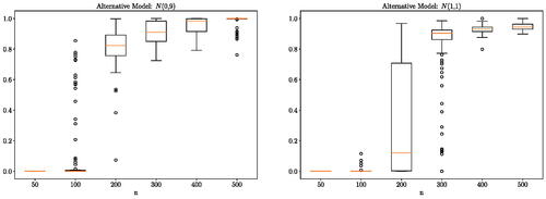
Essentially, when the number of samples is small, there is not enough evidence to determine if the null hypothesis should be rejected. In such a case, the Bayes factor favors the simpler null hypothesis. This is to be expected since Bayesian modeling encompasses a natural Occam factor in the prior predictive (MacKay 2003, chap. 28). We will see this reflected in all the synthetic experiments in this section. Note that for a Gaussian distribution, the difference in mean is easier to detect comparing to a difference in variance. This is reflected in the results presented here and in the supplementary materials: we observe that the probability of the alternative hypothesis becomes very close to 1 at a much smaller sample size for the experiments with a difference in mean.

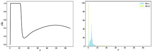
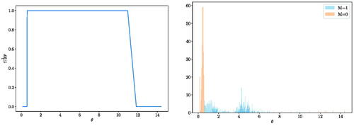
We emphasize that, unlike the frequentist kernel two-sample test where a single value of the lengthscale parameter needs to be predetermined, the proposed Bayesian framework integrates over all possible θ values and alleviates the need for kernel lengthscale selection. However, some θ values are more informative in distinguishing the difference between the two distributions while others are less informative. As a specific example, we consider the case when $P_X=\mathcal{N}(0,1)$ and $P_Y=\mathcal{N}(0,9)$ with 200 samples each. For this specific simulation, we obtain $P(H_1|\mathcal{D})\approx 0.839$. Figure 2 (Left) illustrates the change of the probability of $H_1|\theta ,\mathcal{D}$ as a function of θ. Clearly, the region of θ from approximately 0.05 to 11 is most informative for distinguishing these two distributions. This is also reflected in the marginal distribution of $\theta |H_1$ and $\theta |H_0$ from Figure 2 (Right). Rather than selecting a single lengthscale parameter, the proposed method is able to highlight the range of informative lengthscales. As we will see, this is more useful in cases when multiple lengthscale parameters are of interest for a single testing problem.

Fig. 2 One-dimensional Gaussian experiment with for $P_X=\mathcal{N}(0,1)$ and $P_Y=\mathcal{N}(0,9)$ and 200 samples. Left: The plot illustrates $\frac{1}{1+{\text{BF}}_{\theta }}$ as a function of θ. Right: The histogram of $\theta |M,\mathcal{D}$ for H₁ and H₀.

5.1.2 Laplace Distributions

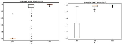
We consider a scenario where the data are generated using the following distributions: $P_X=\mathcal{N}(0,1)$ and $P_Y=\text{Laplace}(0,1.5)$ or $P_Y=\text{Laplace}(0,0.4)$ The results are presented in Figure 3 which aligns with our expectation. As the number of samples increases the test is becoming increasingly certain of the difference between the null and alternative model and hence $P(H_1|\mathcal{D})$ concentrates at 1. Since the proposed method is not restricted to two-sample testing between independent random variables, we also consider the same experiment with correlated standard Gaussian and Laplace distributions generated through copula transformation with correlation set to 0.5. The correlated structure has helped the discovery of the difference between the distributions. Results are presented in supplementary materials illustrating that the method works equally well in correlated random variable cases.

Fig. 3 One-dimensional Laplace experiment: distribution (over 100 independent runs) of the probability of the alternative hypothesis $p(H_1|\mathcal{D})$ for a different number of observations n. Here, $P_X=\mathcal{N}(0,1)$ and $P_Y=\text{Laplace}(0,1.5)$ (Left) or $P_Y=\text{Laplace}(0,0.4)$ (Right).

5.2 Two-by-Two Blobs of 2-Dimensional Gaussian Distributions

The performance of the frequentist kernel two-sample test using MMD depends heavily on the choice of kernel. When a Gaussian kernel is used, this boils down to choosing an appropriate lengthscale parameter. Often, median heuristic is used. However, Gretton et al. (2012b) showed that MMD with median heuristic failed to reject the null hypothesis when comparing samples from a grid of isotropic Gaussian versus a grid of non-isotropic Gaussian. The framework proposed by Flaxman et al. (2016) showed that, by choosing the lengthscale that optimize the Bayesian kernel learning marginal log-likelihood (i.e., an empirical Bayes type of approach), MMD is able to correctly reject the null hypothesis at the desired significance level. Intuitively, the algorithm needs to look locally at each blob to detect the difference rather than at the lengthscale that covers all of the blobs which is given by the median distance between points.

We repeat this experiment using the proposed Bayesian two-sample test with P_X being a mixture of 2-dimensional isotropic Gaussian distributions and P_Y a mixture of 2-dimensional Gaussian distributions centered at slightly shifted locations with rotated covariance matrix. Note, this is not the same dataset used in Flaxman et al. (2016) and Gretton et al. (2012b), we shift the dataset to have multiple relevant lengthscales. We center the blobs of the 2-dimensional Gaussian distributions of P_X at $\mathrm{(}\text{HTML}\mathrm{ }\text{translation}\mathrm{ }\text{failed}\mathrm{)}$ ${(30,10)}^{\top },{(30,30)}^{\top }\}$ and shift such locations by $(-1,-1)$ for P_Y. An equal number of observations is sampled from each of the blobs. The covariance matrix of P_Y follows the form given in the supplementary materials, with $ϵ=\{2,6,10,20\}.$ We present illustrations of the samples from these distributions in the supplementary materials.

Figure 4 shows that our approach is able to detect the difference between the distributions since the probability of the alternative hypothesis becomes more concentrated around 1 as the number of samples increases. Note, when $ϵ=2$, the distribution of the probability of the alternative hypothesis is around 0.6. We expect this to increase to 1 as we increase the number of samples to around 300 samples per blob given the pattern observed.

Fig. 4 2-by-2 blobs of bivariate Gaussian experiment: distribution (over 100 independent runs) of the probability of the alternative hypothesis $p(H_1|\mathcal{D})$ for a different number of observations n. The distribution of X is a mixture of four bivariate Gaussian distributions with equal probability centered at $\{{(10,10)}^{\top },{(10,30)}^{\top },{(30,10)}^{\top },{(30,30)}^{\top }\}$ and with ϵ = 1. The distribution of Y is also a mixture of four bivariate Gaussian distributions with equal probability centered around the same locations but also shifted by $(-1,-1).$ In this experiment, we consider the cases when $ϵ=\{2,6,10,20\}.$

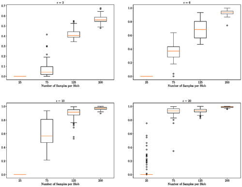
As an example, in Figure 5 (Left), we see that a wide range of lengthscales is informative for this two-sample testing problem when ϵ = 2. If we further observe the marginal distributions $P(\theta |M=0,\mathcal{D})$ and $P(\theta |H_1,\mathcal{D})$ in Figure 5 (Right), the method takes advantage of the large lengthscales to detect shift in location and the small lengthscales to detect the difference in covariance. But when the lengthscale is too small (approximately less than 0.5), the method regards the samples as identically distributed.

Fig. 5 2-by-2 blobs of bivariate Gaussian experiment under the alternative model ϵ = 2 and 200 samples per blob. Left: the plot illustrates $\frac{1}{1+{\text{BF}}_{\theta }}$ against the value of θ. Right: histogram of samples from the marginal distribution of $\theta |M,\mathcal{D}$ for H₁ and H₀.

5.3 Higher Dimensional Gaussian Distributions

We have seen that the proposed method is able to use informative value of the lengthscale parameter and make correct decisions about the probability of the alternative hypothesis given large enough samples. In this section, we investigate the effect of dimensionality of the given sample on the proposed two-sample testing method. We use the Gaussian blobs experiment from the previous section and append simple $\mathcal{N}(0,1)$ to both X and Y (i.e., the difference in distribution exists only in the first two dimensions). In particular, we consider the cases when the total number of dimensions are $\{3,4,5,6,7\}$. The results are presented in Figure 6.

Fig. 6 Higher dimensional experiment: distribution (over 100 independent runs) of the probability of the alternative hypothesis $p(H_1|\mathcal{D})$ for a different number of observations n. For the first two dimensions, the data is generated as in Section 5.2 with ϵ = 6. Standard Gaussian noises are appended as the remaining dimensions. Top left figure is copied from Figure 4 for the ease of performance comparison.

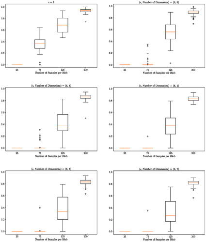
We observe that the test requires more samples to detect the difference between the two distributions as the number of dimension increases. The noise in the additional dimensions has indeed made the problem harder for the given number of samples. But the proposed method still manages to discover the difference as the number of samples increases. For up to eight dimensions, the method returns a posterior probability of H₁ higher than 0.8 as soon as there are more than 200 samples per blob. This illustrates the robustness of our proposed method to the dimensionality of the problem.

5.4 Comparison to other Bayesian Nonparametric Methods

In this section we compare our test to other Bayesian nonparametric two-sample tests in the literature. In particular we compare our method to the two approaches of Chen and Hanson (2014) and Holmes et al. (2015) based on Pólya tree priors. We consider the following setting: $X\stackrel{\text{iid}}{\sim }{P}_X=N(0,1)$ versus $Y\stackrel{\text{iid}}{\sim }{P}_Y=N(\mu ,1)$ with $\mu \in \{0,1.5,3\}$ and a sample size n = 200.

As depicted in Figure 7, one can see that our method correctly returns a posterior probability of H₁ close to 0 under H₀ (μ = 0) and a posterior probability close to 1 under H₁, when $\mu =1.5$ and μ = 3. Similar behavior is displayed for the method of Holmes et al. (2015). However, the test of Chen and Hanson (2014) appears to have posterior probabilities for H₁ which are systematically biased upwards. The problem becomes aggravated with increasing dimension. In Figure 8 we simulate $X\stackrel{\text{iid}}{\sim }{P}_X=N(0,I_D)$ versus $Y\stackrel{\text{iid}}{\sim }{P}_Y=N(0,I_D)$ with $D\in \{1,3,5\}$ and a sample size of n = 100 to see if Chen and Hanson (2014) can correctly identify H₀ in higher dimensions.

Fig. 7 Comparison of our approach (Left) to the methods proposed by Chen and Hanson (2014) (Middle) and Holmes et al. (2015) (Right): distribution (over 100 independent runs) of the posterior probability $p(H_1|\mathcal{D})$ in a one-dimensional setting where $P_X=N(0,1)$ and $P_Y=N(\mu ,1)$ for $\mu \in \{0,1.5,3\}$ with a sample size n = 200.

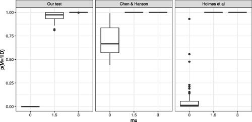
Fig. 8 Comparison of our approach (Left) to the methods proposed by Chen and Hanson (2014) (Right): distribution (over 100 independent runs) of the posterior probability $p(H_1|\mathcal{D})$ in a multi-dimensional setting where $P_X=N(0,I_D)$ and $P_Y=N(0,I_D)$ for $D\in \{0,1.5,3\}$ with a sample size n = 100.

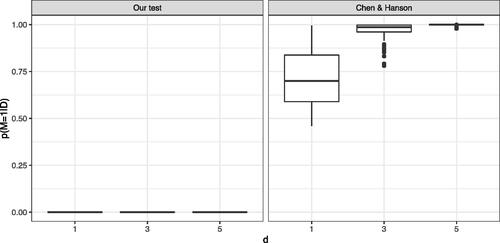
As shown in Figure 8 with increasing dimension, the posterior probability of H₁ becomes closer to one, which means that the test is unable to identify H₀. However, our test correctly identifies H₀ in all dimensions. Presumably to overcome the issue of biased posterior probabilities, Chen and Hanson (2014) do not use their Bayes factor in the classical Bayesian sense. Instead, they use it as a test statistic for a (frequentist) permutation test. The utility of power comparisons between Bayesian and frequentist paradigms is questionable so we do not pursue that direction here. We recall that the test of Holmes et al. (2015) can only handle one-dimensional data. We also note that Holmes et al. (2015) assume that the two underlying distributions are continuous and model them using Polya tree priors. In contrast, kernel-based methods do not require continuity assumptions and can therefore be applied to general distributions.

6 Real Data Experiments

6.1 Network Heterogeneity From High-Dimensional Data

In system biology and medicine, the dynamics of the data under analysis can often be described as a network of observed and unobserved variables, for example a protein signaling network in a cell (Städler and Mukherjee 2019). One interesting problem in this area is to investigate if the signaling pathways (networks) reconstructed from two subtypes are statistically different.

In this section, we follow the statistical setup given in Städler and Mukherjee (2017, 2019) and describes the networks by Gaussian graphical models (GGMs) which use an undirected graph (or network) to describe probabilistic relationships between p molecular variables. Assume that each sample X_i (and similarly for Y_i ) is sampled from a multivariate Gaussian distribution with zero mean and some concentration matrix Ω (i.e., the inverse of a covariance matrix). The concentration matrix defines the graph G via$$(j,j\prime )\in E(G)\iff {\Omega }_{jj\prime }\cancel{=}0$$for $j\cancel{=}j\prime \in \{1,\dots ,p\}$ and E(G) denotes the edge set of graph G. Network homogeneity problem presented in the previous paragraph can be formulated as a two-sample testing problem in statistics where we are interested in testing the null hypothesis(30) $$H_0:G_1=G_2$$(30)

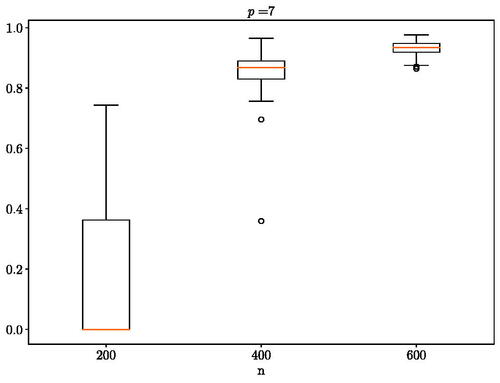
In the first experiment, we use the code from Städler and Mukherjee (2019) to generate a pair of networks with five nodes that present four common edges and then obtain the corresponding correlation matrices to use as the covariance matrices for the multivariate Gaussian distribution. The results are presented in Figure 9. In the second experiment, we again use the code from Städler and Mukherjee (2019) to generate hub networks with seven nodes that are divided into three hubs with one hub that is different and use the obtained correlation matrices in the multivariate Gaussian distribution as with the first experiment. The results are presented in Figure 10. Both tests were able to recover the ground truth as the number of observed sample increases.

Fig. 9 Random networks heterogeneity testing: distribution (over 100 independent runs) of the probability of $H_1|\mathcal{D}$ for a different number of samples.

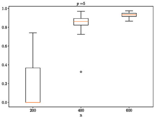
Fig. 10 Hub network heterogeneity testing: distribution (over 100 independent runs) of the probability of $H_1|\mathcal{D}$ for a different number of samples.

6.2 Real Data: Six-Membered Monocyclic Ring Conformation Comparison

In this section, we consider a real world application of our proposed method to detect if the conformation observed in crystal structures differ from its lowest energy conformation in gas phase. Qualitative descriptions are often given to show that the two are distributed differently due to the crystal packing effect. While no quantitative analysis has been provided in the chemistry literature, we aim to perform such analysis through the use of the proposed Bayesian two-sample test.

We use the Cremer–Pople puckering parameters (Cremer and Pople 1975) to describe the six-membered monocyclic ring conformation and compare their shapes under the two different conditions described above. This coordinate system first defines a unique mean plane for a general monocyclic puckered ring. Amplitudes and Phases coordinates are then used to describe the geometry of the puckering relative to the mean plane. For a six-membered monocyclic ring, there are three puckering degrees of freedom, which are described by a single amplitude-phase pair $(q_2,{\varphi }_2)$ and a single puckering coordinate q₃. As we consider general six-membered rings, we can omit the phase parameters ${\varphi }_2$ for simplicity and compare the degree of puckering (maximal out-of-plane deviation) under different conditions. The crystal structures of 1936 six-membered monocyclic rings are extracted from the Crystallography Open Database (COD) and the associated puckering parameters are calculated. Independently, we calculate the lowest energy conformations of a diverse set of 26,405 molecules using a semiempirical method GFN2 and record the puckering parameters. We consider 100 random samples of size $n=\{200,400,600,800\}$ from each of the datasets and conduct our Bayesian two-sample test 100 times while inferring the kernel bandwidth parameter θ.

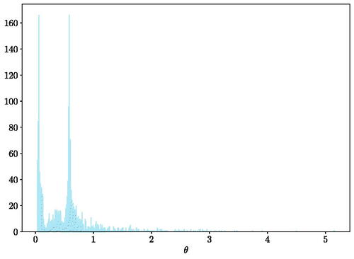
Figure 11 illustrates the results of our test. The proposed method is becoming more certain that the lowest energy conformation in gas phase of six-membered monocyclic rings is distributed differently from its crystal structures as the number of samples increases. At 800 samples, the proposed method gives the probability of $H_1|\mathcal{D}$ equals to 1 which aligns with expert opinions that the two are indeed distributed differently due to the crystal packing effect. In Figure 12, we provide the posterior histogram of $\theta |H_1,\mathcal{D}$ when 800 samples are observed. The frequency distribution is multi-model indicating that multiple lengthscale is of interest for this problem at hand.

Fig. 11 Six-membered monocyclic ring conformation comparison: distribution (over 100 independent runs) of the probability of $H_1|\mathcal{D}$ for a different number of samples.

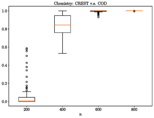
Fig. 12 Histogram of samples from the marginal distribution $\theta |M=1,\mathcal{D}$ for the experiment on six-membered monocyclic ring conformation comparison with 800 samples.

7 Conclusion

In this work, we have proposed a Bayesian two-sample testing framework using the Bayes factor. Rather than directly considering the observations, we have proposed to consider the differences between the empirical kernel mean embeddings (KME) evaluated at a set of inducing points. Following the learning procedure of the empirical KME (Flaxman et al. 2016), we have derived the Bayes factors when the kernel hyperparameter is given as well as when it is treated in a fully Bayesian way and marginalized over. Further, we have obtained efficient computation methods for the marginal pseudolikelihood using the Kronecker structure of the covariance matrices. The posterior inference of the model label and the kernel hyperparameter is done by HMC within Gibbs. We have showed in a range of synthetic and real experiments that our proposed Bayesian test is able to simultaneously using multiple lengthscales and correctly uncover the ground truth given sufficient data.

Following this work, there are several possible directions for future research. We have seen in Section 5 that larger sample sizes are required for more challenging problems. A random Fourier feature approximation of the above framework can be easily developed to enable the use of large sample size without having prohibitive runtime. In this case, explicit finite dimensional feature maps are available, the difference between the mean embeddings $\delta ={\mu }_X-{\mu }_Y$ can be written more explicitly as $\delta =\mathbb{E}(\varphi (X))-\mathbb{E}(\varphi (Y))$. Assume a GP prior with an appropriate covariance matrix for δ, $\varphi (x_i)-\varphi (y_i)$ can be modeled by a Gaussian distribution with mean $\mathbb{E}(\varphi (X))-\mathbb{E}(\varphi (Y))$ and covariance estimated as presented in the supplementary materials. While the rest of the inference procedure can follow similarly as presented here, this large scale approximation requires careful specification of the covariance matrix for the GP model of δ to ensure that draws from such GP lie in the correct RKHS.

Recently, Kamary et al. (2014) proposed a mixture modeling framework for Bayesian model selection. The authors argues that the mixture modeling framework provides a more thorough assessment of the strength of the support of one model against the other and allows the use of noninformative priors for model parameters when the two competing hypotheses share the same set of parameters which is prohibitive in the classical Bayesian two-sample testing approach like Bayes factor (DeGroot 1973). The proposed Bayesian two-sample testing framework using Bayes factor can be equivalently formulated as a mixture model:$$\Delta |\theta ,\pi \sim \pi N(0,\frac{1}{n}{\Sigma }_{\theta })+(1-\pi )N(0,R_{\theta }+\frac{1}{n}{\Sigma }_{\theta }).$$

The posterior distribution of the mixture proportion $0\le \pi \le 1$ indicates the model preferred. A joint inference of π and the kernel bandwidth parameter θ can be easily done through MCMC. It would be interesting to see if there is a difference in performance between the mixture approach and the Bayes factor approach proposed here. Finally, the Bayesian testing framework developed here and the directions for future work can all be applied to independence testing.

Code for the proposed method and experiments is available at: https://github.com/qinyizhang/BayesianKernelTesting

Acknowledgments

The authors thank Lucian Chan for helping with the chemistry data and Chris Holmes whose advice in the early stages of the project was instrumental in shaping its direction.

Supplementary Materials

The supplementary materials provides details on derivation, proofs, and additional synthetic data experiments.

Additional information

Funding

Q. Z. was supported by the Engineering and Physical Sciences Research Council (EPSRC) (EP/M50659X/1).

References

- Berlinet, A., and Thomas-Agnan, C. (2004), Reproducing Kernel Hilbert Spaces in Probability and Statistics, Dordrecht: Kluwer.
- Bernardo, J. M., and Smith, A. F. M. (2000), Bayesian Theory, Chichester: Wiley.
- Borgwardt, K. M., and Ghahramani, Z. (2009), “Bayesian Two-Sample Tests,” ArXiv e-prints: 0906.4032.
- Borgwardt, K. M., Gretton, A., Rasch, M. J., Kriegel, H. P., Schölkopf, B., and Smola, A. J. (2006), “Integrating Structured Biological Data by Kernel Maximum Mean Discrepancy,” Bioinformatics, 22, 49–57. DOI: 10.1093/bioinformatics/btl242.
- Carpenter, B., Gelman, A., Hoffman, M. D., Lee, D., Goodrich, B., Betancourt, M., Brubaker, M., Guo, J., Li, P., and Riddell, A. (2017), “Stan: A Probabilistic Programming Language,” Journal of Statistical Software, 76, 1–32. DOI: 10.18637/jss.v076.i01.
- Chen, Y., and Hanson, T. E. (2014), “Bayesian Nonparametric k-Sample Tests for Censored and Uncensored Data,” Computational Statistics & Data Analysis, 71, 335–346.
- Cremer, D., and Pople, J. A. (1975), “General Definition of Ring Puckering Coordinates,” Journal of the American Chemical Society, 97, 1354–1358. DOI: 10.1021/ja00839a011.
- DeGroot, M. H. (1973), “Doing What Comes Naturally: Interpreting a Tail Area as a Posterior Probability or as a Likelihood Ratio,” Journal of the American Statistical Association, 68, 966–969. DOI: 10.1080/01621459.1973.10481456.
- Filippi, S., and Holmes, C. C. (2016), “A Bayesian Nonparametric Approach to Testing for Dependence Between Random Variables,” Bayesian Analysis, Advance Publication. DOI: 10.1214/16-BA1027.
- Filippi, S., Holmes, C. C., and Nieto-Barajas, L. E. (2016), “Scalable Bayesian Nonparametric Measures for Exploring Pairwise Dependence via Dirichlet Process Mixtures,” Electronic Journal of Statistics, 10, 3338–3354. DOI: 10.1214/16-ejs1171.
- Flaxman, S., Sejdinovic, D., Cunningham, J. P., and Filippi, S. (2016), Bayesian Learning of Kernel Embeddings,” in Uncertainty in Artificial Intelligence (UAI), pp. 182–191.
- Fukumizu, K., Gretton, A., Sun, X. H., and Schölkopf, B. (2008), “Kernel Measures of Conditional Dependence,” in Advances in Neural Information Processing Systems (NIPS).
- Gretton, A., Borgwardt, K., Rasch, M. J., Schölkopf, B., and Smola, A. (2012a), “A Kernel Two-Sample Test,” Journal of Machine Learning Research (JMLR), 13, 723–773.
- Gretton, A., Sriperumbudur, B., Sejdinovic, D., Strathmann, H., Balakrishman, S., Pontil, M., and Fukumizu, K. (2012b), “Optimal Kernel Choice for Large-Scale Two-Sample Tests,” Advances in Neural Information Processing Systems (NIPS).
- Hoffman, M. D., and Gelman, A. (2014), “The no-u-turn Sampler: Adaptively Setting Path Lengths in Hamiltonian Monte Carlo,” Journal of Machine Learning Research, 15, 1593–1623.
- Holmes, C. C., Caron, F., Griffin, J. E., and Stephens, D. A. (2015), “Two-Sample Bayesian Nonparametric Hypothesis Testing,” Bayesian Analysis, 10, 297–320. DOI: 10.1214/14-BA914.
- Jefferys, W. H., and Berger, J. O. (1992), “Ockham’s Razor and Bayesian Analysis,” American Journal of Science, 80, 64–72.
- Jeffreys, H. (1935), “Some Tests of Significance, Treated by the Theory of Probability,” Proceedings of the Cambridge Philosophy Society, 31, 203–222. DOI: 10.1017/S030500410001330X.
- Jeffreys, H. (1961), Theory of Probability, Oxford: Oxford University Press.
- Kamary, K., Mengersen, K., Robert, C. P., and Rousseau, J. (2014), “Testing Hypotheses via a Mixture Estimation Model,” ArXiv e-prints: 1412.2044.
- Kass, R. E., and Raftery, A. E. (1995), “Bayes Factors,” Journal of the American Statistical Association, 90, 773–795. DOI: 10.1080/01621459.1995.10476572.
- Lukić, M. N., and Beder, J. H. (2001), “Stochastic Processes with Sample Paths in Reproducing Kernel Hilbert Spaces,” Transaction of the American Mathematical Society, 353, 3945–3969. DOI: 10.1090/S0002-9947-01-02852-5.
- MacKay, D. J. C. (2003), Information Theory, Inference, and Learning Algorithms, Cambridge: Cambridge University Press.
- Shawe-Taylor, J., and Cristianini, N. (2004), Kernel Methods for Pattern Analysis (Vol. 19 of 22), Cambridge: Cambridge University Press.
- Smola, A., Gretton, A., Song, L., and Schölkopf, B. (2007), “A Hilbert Space Embedding for Distributions,” in Proceedings of the 18th International Conference on Algorithmic Learning Theory, pp. 13–31.
- Sriperumbudur, B. K. (2010), “Reproducing Kernel Space Embeddings and Metrics on Probability Measures,” PhD Thesis, University of California–San Diego.
- Städler, N., and Mukherjee, S. (2017), “Two-Sample Testing in High Dimensions,” Journal of Royal Statistical Society Statistical Methodology, Series B, 79, 225–246. DOI: 10.1111/rssb.12173.
- Städler, N., and Mukherjee, S. (2019), “A Bioconductor Package for Investigation of Network Heterogeneity From High-Dimensional Data,” Available at https://www.bioconductor.org/packages/release/bioc/vignettes/nethet/inst/doc/nethet.pdf.
- Stegle, O., Denby, K. J., Cooke, E. J., Wild, D. L., Ghahramani, Z., and Borgwardt, K. M. (2010), “A Robust Bayesian Two-Sample Test for Detecting Intervals of Differential Gene Expression in Microarray Time Series,” Journal of Computational Biology, 17, 355–367. DOI: 10.1089/cmb.2009.0175.
- Steinwart, I., and Christmann, A. (2008), Support Vector Machines, New York: Springer.
- Wahba, G. (1990), Spline Models for Observational Data, Philadelphia, PA: Society for Industrial and Applied Mathematics.