Statistical Analysis of Locally Parameterized Shapes

Abstract

In statistical shape analysis, the establishment of correspondence and defining shape representation are crucial steps for hypothesis testing to detect and explain local dissimilarities between two groups of objects. Most commonly used shape representations are based on object properties that are either extrinsic or noninvariant to rigid transformation. Shape analysis based on noninvariant properties is biased because the act of alignment is necessary, and shape analysis based on extrinsic properties could be misleading. Besides, a mathematical explanation of the type of dissimilarity, for example, bending, twisting, stretching, etc., is desirable. This work proposes a novel hierarchical shape representation based on invariant and intrinsic properties to detect and explain locational dissimilarities by using local coordinate systems. The proposed shape representation is also superior for shape deformation and simulation. The power of the method is demonstrated on the hypothesis testing of simulated data as well as the left hippocampi of patients with Parkinson’s disease and controls. Supplementary materials for this article are available online.

Keywords:

• Local coordinate system
• Local dissimilarity
• Parkinson’s disease
• Shape alignment
• Skeletal representation
• s-Rep hypothesis testing

1 Introduction

In statistical shape analysis, detecting and characterizing locational differences between two groups of objects is a matter of special interest. For instance, in medical applications, analysis of shape dissimilarities has the power to shed light on organ deformations, supporting diagnosis and treatment.

Detecting locational differences is a challenging task. For decades, medical researchers have been trying to answer four common questions when comparing a specific organ of a group of patients versus a control group (CG). 1. Existence: Is there any local dissimilarity? 2. Location: What is the location of the dissimilarity? 3. Intensity: What is the size of the dissimilarity? 4. Type: What is the type or interpretation of the dissimilarity (e.g., bending, twisting, or elongation)? Since a dissimilarity can be seen as a distance between two entities, each shape analysis method introduces distances between objects’ corresponding parts (i.e., local dissimilarities) based on a specific shape representation to answer these questions. The shape representation could be invariant or noninvariant to object rigid transformation (i.e., translation and rotation). Therefore, as Lele and Richtsmeier (2001) discussed, roughly we can categorize shape analysis methods into alignment-independent and alignment-dependent approaches that we call invariant and noninvariant methods, respectively. Invariant methods use invariant shape representations to follow the principle of invariance (Berger 1985) based on the fact that the true form of an organism does not change if it translates or rotates. In contrast, noninvariant methods follow the idea of Kendall (1977) to factor out translation, rotation, and (occasionally) scaling from noninvariant shape representations by alignment. Usually, noninvariant methods are more straightforward, faster, and provide a better intuition than invariant methods, which explains their popularity. In comparison, invariant methods are more reliable because they are independent of choosing the alignment method or the coordinate system.

In this work, we propose an invariant method equipped with an invariant shape representation that benefits from the advantages of both types of methods. Further, it answers all the four above questions in a single framework. For this, we locally reparameterize a noninvariant skeletal representation (s-rep) (Pizer et al. 2013) to an entirely invariant shape representation. To better understand and highlight the advantages of our approach, first we need to review other methods in more detail.

Given two groups of objects, in the most common approaches, whether invariant or noninvariant, researchers try to answer the above questions by hypothesis testing based on the following steps. Step 1: Introduce shape representation as a tuple of corresponding geometric object properties (GOPs) among objects. Step 2: Defining a distance between the corresponding GOPs of the two groups known as a test statistic representing the local dissimilarity. Step 3: Measuring and analyzing the test statistics to find significant GOPs. Step 4: Applying multiple testing methods to control false positives.

A GOP can be a geometric or spatial feature (e.g., point’s position, surface normal direction, Gaussian curvature, etc.), a combination of features and their correlations (Tabia and Laga 2015), or more general a local descriptor as discussed in (Laga et al. 2018, Ch.5). A GOP may or may not be invariant to object translation and rotation. We call a shape representation invariant if all of its GOPs are invariant, otherwise noninvariant. Examples of noninvariant shape representations are the point distribution model (PDM) and the discrete s-rep (ds-rep). A PDM consists of an n-tuple of points $({\mathit{x}}_1,\dots ,{\mathit{x}}_n)$, ${\mathit{x}}_i\in {\mathbb{R}}^d$ distributed on or inside a d-dimensional object where d = 2, 3 as comprehensively discussed in Srivastava and Klassen (2016), Jermyn et al. (2017), Laga et al. (2018), and Dryden and Mardia (2016). Thus, the GOPs in a PDM are the points’ Cartesian coordinates. A ds-rep (Pizer et al. 2013) consists of a tuple of directions, tail positions and lengths of a set of internal vectors and will be discussed in further detail in Section 2.1. A ds-rep is partly invariant as the vectors’ lengths are invariant. An example for an invariant shape representation is to convert a PDM to Euclidean distance matrix (EDM) representation as a tuple of pairwise Euclidean distances of points (Lele and Richtsmeier 2001).

Having two groups of shape representations, we can define hypothesis tests based on the corresponding GOPs. In other words, we simply test two groups of tuples element-wise. Note that it is necessary to factor out translation and rotation from noninvariant GOPs by alignment before the analysis. We say the analysis is invariant if the shape representation is invariant, otherwise it is noninvariant. For example, Styner et al. (2006) and Schulz (2013) methods are noninvariant as Styner et al. (2006) compared PDMs of brain objects of patients with schizophrenia v.s. CG, and Schulz (2013) compared the objects’ ds-reps. In contrast, Lele and Richtsmeier (1991) approach is invariant as they used EDM representations to study skull abnormality of patients with Crouzon and Apert syndromes. We briefly discuss both invariant and noninvariant methods by an example.

Figure 1(a) illustrates two ellipsoidal objects as defined in Section 2.1.2, where the left one is an ellipse, and the right one is a bent ellipse. The objects can be seen as an open arm (left one) and a closed arm (right one), where each arm consists of three parts, namely the upper arm, elbow, and forearm. Since the closed arm is a locally deformed version of the open arm, we consider the main difference at the elbow, which is compatible with our visual inspection. Both shapes are manually registered with 20 corresponding boundary points depicted by circles and crosses. By adding independent random noise to each point, we simulated 15 PDMs for each object, as depicted in Figure 1(b). Since a PDM is noninvariant, alignment is necessary.

Fig. 1 Problem of false positives due to alignment. (a) Two ellipsoidals are depicted by line and dashed line. Circles and crosses show corresponding boundary points. Bold points are shapes’ centroids. (b) Two populations of simulated PDMs. (c), (d), (e) Separation of corresponding local distributions.

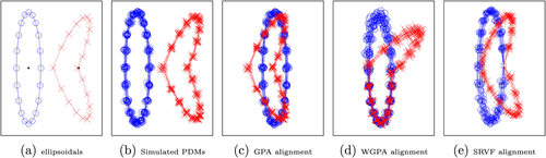
From several available alignment methods, we choose generalized Procrustes analysis (GPA), weighted GPA (WGPA) (Dryden and Mardia 2016), and square root velocity framework (SRVF) (Srivastava and Klassen 2016). Figure 1(c)–(e) illustrate alignments based on GPA, WGPA, and SRVF, respectively. Apparently, there are two main issues. First, the outcomes of different alignment methods are remarkably different as each method tries to minimize a specific type of distance. Thus, choosing the superior alignment method is challenging. Second, detecting locational dissimilarities could be extremely biased because alignment affects the distributions of noninvariant GOPs of points’ positions. As a result, PDM analysis introduces false positives and false negatives. In Figure 1(c), WGPA (based on a manually defined covariance matrix) reduces the variation of forearm GOPs and increases the variation of upper arm GOPs. Similarly, the right point at the elbow in Figure 1(e) has a remarkably smaller GOP variation in comparison with other points. Based on these types of observations, Lele and Richtsmeier (2001) explained why noninvariant methods are biased and why invariant methods are more reliable. However, also for invariant methods a local dissimilarity can lead to false positives and false negatives. For instance, if we convert each PDM of our example to an invariant shape representation, where GOPs are invariant Euclidean distances between points and the centroid of the PDM (i.e., center of gravity $\overline{\mathit{x}}=\frac{1}{n}{\sum }_{i=1}^n{\mathit{x}}_i$ depicted by bold points in Figure 1(a)), then almost all the GOPs in our example become significantly different. Note, in this example, the GOPs are defined as extrinsic distances between the points and the extrinsic centroid. If the centroid as well as the distances to the centroid are defined intrinsic (e.g., by barycentroid (Rustamov, Lipman, and Funkhouser 2009)), no differences would be detected. To some extent, the same discussion is valid for EDM analysis (EDMA) as discussed in supplementary material (SUP). Besides, when we consider only invariant GOPs, it is not always easy to map various analysis results from the feature space to the object space (Jermyn et al. 2017, 6). Consequently, some fundamental aspects of shape analysis, such as mean shape, are unattainable. For instance, it is easy to calculate the EDM of a point-based model like a PDM, but it is difficult or sometimes impossible to reconstruct the model based on its EDM. We have the same situation in persistent homology methods (Gamble and Heo 2010; Turner, Mukherjee, and Boyer 2014) where the information of the persistent diagram is not convertible to the object space.

In summary, on the one hand, noninvariant methods are biased due to alignment, and on the other hand, invariant methods based on extrinsic properties could be misleading. Thus, from our point of view, a suitable method should be invariant, based on intrinsic object properties, ensure good correspondence between the GOPs, and be able to answer the fourth question, that is, to provide a mathematical (and medical) interpretation of the type of dissimilarity such as bending, twisting, stretching, protrusion, etc. For example, boundary PDMs cannot explain the local bending in closed arms. In contrast, a skeletal model (see Figure 2(a)) can explain the bending mathematically, as we will discuss in Section 2.4. However, the main obstacle in the skeletal analysis is the definition of correspondence.

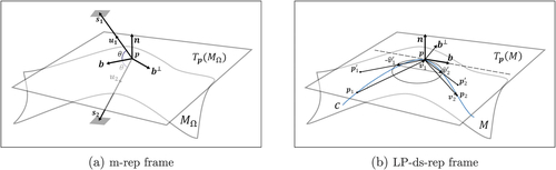
Fig. 2 Skeletal structure of ellipsoidal objects. (a) 2D m-reps. s and $\mathit{s}\prime$ are corresponding spokes with unit directions u and $\mathit{u}\prime$. (b) A fitted ds-rep to a left hippocampus’s mesh including up, down, crest spokes, and the skeletal sheet.

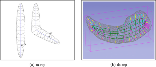
For a specific class of ellipsoidal objects, Pizer et al. (2013) introduced s-rep and defined correspondence based on its discrete version ds-rep (see Figure 2(b)). As pointed out above, ds-reps are noninvariant and thus might bias the analysis. Further, ds-rep analysis is able to identify only a few types of dissimilarities, for example, protrusion or bending. The identification of other types remains challenging. To overcome these limitations, we propose a novel hierarchical ds-rep parameterization based on local coordinate systems known as local frames. The proposed hierarchical local parameterization of ds-rep, called LP-ds-rep, is an invariant shape representation which supports sensitive hypothesis testing, that is, not biased by alignment. Note that the hierarchical structure equipped with local frames can be modified and fit to any kind of objects (not only ellipsoidals) as long as a robust tree structure can be established for the shape model. This is the subject of further studies.

The article is structured as follows. In Section 2, we first review basic notations and amenities of s-reps and discuss the conventional noninvariant definition of ds-rep with the discussed challenges. Then, in Sections 2.1.3 and 2.1.4, we propose the novel LP-ds-rep parameterization. Further, we explain the euclideanization of spherical data, mean shape, the transformation between two parameterizations, skeletal deformation, and simulation. Section 3 introduces a hypothesis test method and discusses controlling false positives. In Section 4 we study hippocampal differences between a group of patients with Parkinson’s disease and CG. Besides, we compare the results of both parameterizations plus EDMA and show the advantages of our method on simulated data. Finally, we summarize and conclude the work in Section 5. A flowchart depicting the framework of the presented methods can be found in the SUP.

2 Skeletal Representation

To understand skeletal representation, we need to review some fundamental definitions.

In this work, the set $\Omega \subset {\mathbb{R}}^d$ is a d-dimensional (or dD) object if it is homeomorphic to the d-dimensional closed ball, where d = 2, 3. We denote the boundary and the interior of Ω, by $\partial \Omega$ and Ω_in , respectively. Thus, $\Omega =\partial \Omega \cup {\Omega }_{in}$. Also, we consider only objects with smooth boundaries. Therefore, $\partial \Omega$ is a closed connected genus-zero smooth surface if d = 3, and it is a smooth closed curve if d = 2 (Jermyn et al. 2017, Ch.2). The medial locus of Ω is a collection of entirely connected curves or sheets in Ω_in forming the centers of all maximal inscribed spheres bi-tangent or multi-tangent to $\partial \Omega$. We denote the medial locus of Ω by $M_{\Omega }$. The skeleton of Ω is any curve or sheet from which non-crossing spokes to $\partial \Omega$ emanate at each point of it. Note that a spoke is a vector whose tail is on the object’s skeleton, and its tip is on $\partial \Omega$. We consider a skeletal of an object as a set of all non-crossing spokes emanating from its skeleton. Thus, the skeletal can be seen as a field of spokes on the skeleton. The medial locus is a form of skeleton where medial spokes connecting the center of maximal inscribed spheres to their tangency points. The union of the medial spokes forms the medial skeletal (Siddiqi and Pizer 2008).

Medial representation (m-rep) and its properties have been extensively studied in the literature (Pizer et al. 1999; Fletcher et al. 2004; Siddiqi and Pizer 2008). Figure 2(a) illustrates m-reps of two ellipsoidal objects. Briefly, an m-rep is a discrete medial skeletal (i.e., finite set of medial spokes). Thus, an m-rep reflects the interior object properties such as local widths and directions. However, as pointed out in (Pizer et al. 2013), the m-rep is sensitive to boundary noise because every protruding boundary kink results in additional medial branches. This sensitivity affects m-rep correspondence among a population as two versions of the same objects can result in significantly different m-reps. Thus, Pizer et al. (2013) relaxed the medial conditions and defined s-rep for a class of ellipsoidal objects like hippocampus (discussed in detail in Section 2.1.2) as a penalized version of m-rep. As Liu et al. (2021) described, the s-rep of 3D ellipsoidal object Ω has the form (M, S), where skeleton $M\subset {\Omega }_{in}$ known as skeletal sheet is a smooth 2-disk (i.e., an embedded, oriented two-dimensional manifold of genus-zero with a single boundary component), and skeletal S is the field of noncrossing spokes on M. The field S consists of three distinct fields of spokes: S₀ along M₀ where M₀ is the boundary of M, $S_{+}$ (respectively, $S_{-}$) defined on the relative interior of M, agreeing (respectively, disagreeing) with the orientation of M. Thus, $S_{+}$ and $S_{-}$ map $M\setminus M_0$ to two sides of $\partial \Omega$ considered as northern and southern part, and S₀ maps M₀ to the crest of $\partial \Omega$. We call a spoke s an up spoke, down spoke, or crest spoke if it belongs to $S_{+},S_{-}$, or S₀, respectively. The same definition is applicable for 2D objects where M is a smooth open curve. The relaxed conditions assure stability in the branching structure and thus good case-to-case correspondence across a population of s-reps. The ds-rep is a discrete form of s-rep (i.e., a finite set of spokes). The conventional ds-rep parameterization is noninvariant as explained in more detail in Section 2.1.1. Afterward, the proposed invariant parameterization based on a hierarchical structure of the local frames is introduced. Also, we name the conventional parameterization as globally parameterized ds-rep (GP-ds-rep), and the new parameterization as locally parameterized ds-rep (LP-ds-rep). Further, $s^{\text{GP}}$ and $s^{\text{LP}}$ denote GP-ds-rep and LP-ds-rep, respectively.

2.1 Parameterizations

2.1.1 GP-ds-rep

There are different ways to fit and parameterize a GP-ds-rep. Depending on the method of model fitting, for example, (Liu et al. 2021), some spokes may share a common tail position (see Figure 2(b)). Let n_s be the number of spokes, and n_p be the number of tail positions s.t. $n_p\le n_s$. A GP-ds-rep can be seen as a tuple $s^{\text{GP}}={({\mathit{p}}_j,{\mathit{u}}_i,r_i)}_{i,j}=({\mathit{p}}_1,\dots ,{\mathit{p}}_{n_p},{\mathit{u}}_1,\dots ,{\mathit{u}}_{n_s},r_1,\dots ,r_{n_s})$ where $\forall j\in \{1,\dots ,n_p\}$: ${\mathit{p}}_j\in {\mathbb{R}}^3$ is jth spoke’s tail position, $\forall i\in \{1,\dots ,n_s\}$: ${\mathit{u}}_i\in {\mathbb{S}}^2$, and $r_i\in {\mathbb{R}}^{+}$ are ith spoke’s direction, and length, respectively. Note ${\mathbb{S}}^d=\{\mathit{x}\in {\mathbb{R}}^{d+1}| \left|\right|\mathit{x}\left|\right|=1\}$ is the unit d-sphere where $d\in \mathbb{N}$. From now on we assume $i=1,\dots ,n_s$ and $j=1,\dots ,n_p$.

The set ${\left\{{\mathit{p}}_j\right\}}_{j=1}^{n_p}$ forms an $n_p\times 3$ configuration matrix P representing the skeletal PDM. Let $I_{n_p}$ be the $n_p\times n_p$ identity matrix and ${\mathit{1}}_{n_p}$ be the $n_p\times 1$ vector of ones. Location and scale can be removed by centering and normalizing P to obtain the pre-shape $\tilde{P}=\frac{C_{n_p}P}{\left|\right|C_{n_p}P\left|\right|}$, where $C_{n_p}=I_{n_p}-\frac{1}{n_p}{\mathit{1}}_{n_p}{\mathit{1}}_{n_p}^T$ is the centering matrix, and $\left|\right|X\left|\right|=\sqrt{\text{trace}(X^{T}X)}$ is the Euclidean norm. Since $\left|\right|\tilde{P}\left|\right|=1$, the pre-shape $\tilde{P}$ lives on the hypersphere ${\mathbb{S}}^{3n_p-1}$ (Pizer et al. 2013). Therefore, a GP-ds-rep lives on a manifold as a direct product of Riemannian symmetric spaces ${\mathbb{S}}^{3n_p-1}\times {({\mathbb{S}}^2)}^{n_s}\times {\mathbb{R}}_{+}^{n_s+1}$ where ${\mathbb{S}}^{3n_p-1}$ indicates the pre-shape space of the skeletal positions, ${({\mathbb{S}}^2)}^{n_s}$ is the space of n_s spokes’ directions, and ${\mathbb{R}}_{+}^{n_s+1}$ is the space of spokes’ lengths and the scaling factor. As we mentioned before, spoke positions and directions are noninvariant as they are in a global coordinate system (GCS). Thus, ds-rep analysis based on this representation is biased.

For m-rep, a semi-local parameterization was proposed by Fletcher, Lu, and Joshi (2003) based on local frames $(\mathit{n},\mathit{b},{\mathit{b}}^{\perp })\in SO(3)$, where n is normal to the medial locus $M_{\Omega }$ at $\mathit{p}\in M_{\Omega }$, $\mathit{b}=\frac{{\mathit{u}}_1+{\mathit{u}}_2}{\left|\right|{\mathit{u}}_1+{\mathit{u}}_2\left|\right|}$ is the bisector direction of two equal-length spokes with common position, ${\mathit{b}}^{\perp }=\mathit{n}\times \mathit{b}$, and SO(3) is the 3D rotation group. Spokes’ directions are defined relative to the local frames by the angle $\theta \in [0,\pi )$ between b and the spokes (see Figure 5(a)). Because the direction of b and ${\mathit{b}}^{\perp }$ depends on the spokes’ directions, if $\theta =\frac{\pi }{2}$ then b takes an arbitrary direction that violates the uniqueness and consistency of the fitted frame. Besides, the spokes’ tail positions and frame directions are noninvariant as they are in GCS.

Inspired by Cartan’s moving frames on space curves (Cartan 1937) and Fletcher’s semi-local parameterization, we propose a fully local ds-rep parameterization. By uisng the inherent hierarchical structure of ds-reps, we provide a consistent definition of local frames independent of GCS that avoids arbitrary frame rotation. This can be done by introducing a leaf-shaped skeletal structure for ellipsoidal objects, that is, reflected in (Liu et al. 2021) (see Figure 6 on page 7). For this, we need to discuss ellipsoidal objects.

2.1.2 Ellipsoidal Objects

Intuitively, an object is ellipsoidal if its skeletal structure corresponds to the skeletal of an eccentric ellipsoid (i.e., ellipsoid with unequal principal radii).

Let ${\mathcal{E}}_3\subset {\mathbb{R}}^3$ be a 3D eccentric ellipsoid. The medial locus of ${\mathcal{E}}_3$ is a 2D ellipsoid (i.e., an ellipse) ${\mathcal{E}}_2\subset {\mathbb{R}}^2$ that we call medial ellipse. The medial locus of ${\mathcal{E}}_2$ is a 1D ellipsoid (i.e., a line segment) ${\mathcal{E}}_1\subset {\mathbb{R}}^1$ that we call medial line. The medial locus of ${\mathcal{E}}_1$ is a 0D ellipsoid (i.e., a point) ${\mathcal{E}}_0\subset {\mathbb{R}}^0$ that we call medial centroid. Thus, $M_{{\mathcal{E}}_n}={\mathcal{E}}_{n-1}$ is the medial locus of ${\mathcal{E}}_n$ where n = 1, 2, 3. 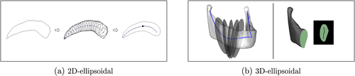Analogous to backward principal component analysis (PCA) (Damon and Marron 2014), we consider ${\mathcal{E}}_3$, ${\mathcal{E}}_2,{\mathcal{E}}_1$, and ${\mathcal{E}}_0$ as four principal ellipsoids (see Figure 4(Left)).

We call a 2D object a perfect 2D-ellipsoidal if its medial locus is a smooth open curve that we call medial curve (see Figures 2a and 3a). Let ${\Omega }_2$ be a perfect 2D-ellipsoidal with medial locus $M_{{\Omega }_2}$. Since $M_{{\mathcal{E}}_2}$ (i.e., medial line ${\mathcal{E}}_1$) is also a smooth open curve, we can define correspondence between $M_{{\mathcal{E}}_2}$ and $M_{{\Omega }_2}$ based on (Srivastava and Klassen 2016). We consider a point on $M_{{\Omega }_2}$ corresponding to ${\mathcal{E}}_0$ as the medial centroid of ${\Omega }_2$. Let γ represent the medial locus $M_{{\Omega }_2}$ (or $M_{{\mathcal{E}}_2}$) based on curve length parameterization l. We know that for each medial point $\gamma (l)$, there are two medial spokes, one for each side of the medial locus, with tail on $\gamma (l)$ and tip ${\gamma }^{\pm }$ on the object boundary at(1) $${\gamma }^{\pm }=\gamma (l)-\mathit{R}(l)|\frac{d}{dl}\mathit{R}(l)|\mathit{t}\pm \mathit{R}(l)\sqrt{1-|\frac{d}{dl}\mathit{R}(l){|}^2}\mathit{n},$$(1) where n and t are normal and tangent vectors of the medial locus at $\gamma (l)$, and $\mathit{R}$ is the radius function such that $\mathit{R}(l)$ is the radius of the maximal inscribe sphere centered at $\gamma (l)$ (Siddiqi and Pizer 2008, Ch.2). Note that the two spokes at the edge (i.e., endpoints) of the medial locus coincide. Thus, in addition to the medial locus, the medial skeletal of ${\Omega }_2$ corresponds to the medial skeletal of ${\mathcal{E}}_2$.

Fig. 3 (a) Illustration of a 2D-ellipsoidal (left) approximated by a perfect 2D-ellipsoidal (right). The solid curve and the bold dot (right) depict the medial curve and medial centroid, respectively. (b) Left: A mandible (without coronoid processes) as an example of a 3D-ellipsoidal with slicing planes. The solid curve is the center curve. Right: A cross-section as a 2D-ellipsoidal including its medial curve.

We say a 2D object ${\widehat{\Omega }}_2$ is 2D-ellipsoidal if its boundary can be precisely approximated¹ by the boundary of a perfect 2D-ellipsoidal ${\Omega }_2$. Following m-rep idea of Pizer et al. (1999), it is reasonable to consider the skeletal of ${\widehat{\Omega }}_2$ as the skeletal of ${\Omega }_2$ to have a better correspondence among a population. Thus, we assume $M_{{\Omega }_2}$ as the skeleton of ${\widehat{\Omega }}_2$ as depicted in Figure 3(a). In 3D, we define 3D-ellipsoidal analogous to generalized offset surface.

Damon (2008) defined generalized offset surfaces as 3D objects similar to generalized tubes² based on sequences of affine slicing planes (not necessarily parallel) such that the cross-sections of a generalized offset surface (i.e., the intersection of the slicing planes with the object) do not intersect within the object, and the boundary of the cross-sections forms the object’s boundary. The skeleton of a generalized tube is a smooth curve, and the skeleton of a generalized offset surface is a smooth two-disk. In practice, we can represent a generalized tube or an offset surface by a finite but large number of disjoint cross-sections. Similarly, we say an object is 3D-ellipsoidal if it can be represented by a large number of disjoint cross-sections such that all the cross-sections are 2D-ellipsoidals, and the length of a curve called the center curve connecting the medial centroids of the successive cross-sections is remarkably larger than the length of the medial curve of each cross-section. Since the union of the medial curves can be seen as a discrete skeletal sheet, Pizer et al. (2013) realized such 3D-ellipsoidals as slabular³ and introduced (slabular) ds-reps such that for a slabular, the implied boundary of its ds-rep (i.e., envelope of the spokes’ tips) approximates the slabular’s boundary. Examples of 3D-ellipsoidals are mandible (without considering the coronoid processes), caudate nucleus, kidney, and hippocampus. Figure 3(b) illustrates the center curve and the slicing planes of a mandible as a 3D-ellipsoidal (left) and a cross-section as a 2D-ellipsoidal (right).

Any eccentric ellipsoid ${\mathcal{E}}_3$ can be seen as a 3D-ellipsoidal such that parallel cross-sections are perpendicular to the center curve (i.e., the major axis of ${\mathcal{E}}_2$). In this sense, a meaningful correspondence⁴ between the skeletal of a 3D-ellipsoidal and skeletal of ${\mathcal{E}}_3$ is assumable as the skeleton of both of them consists of a center curve, a set of medial curves emanating from the center curves, and two spokes at each point of the medial curves pointing toward two sides of the skeletal sheet based on Equation (1)(1) $${\gamma }^{\pm }=\gamma (l)-\mathit{R}(l)|\frac{d}{dl}\mathit{R}(l)|\mathit{t}\pm \mathit{R}(l)\sqrt{1-|\frac{d}{dl}\mathit{R}(l){|}^2}\mathit{n},$$(1) . However, obtaining such correspondence is difficult as it is challenging to define corresponding cross-sections for a population of c-shape objects, for example, a set of hippocampi.

A possible approach for defining a skeletal sheet of a 3D-ellipsoidal is to understand the object via a diffeomorphism from a reference 3D-ellipsoidal such as ${\mathcal{E}}_3$. Assume ${\Omega }_3$ be a 3D-ellipsoidal. Since ${\mathcal{E}}_3$ as a reference object is a 3D-ellipsoidal and a meaningful correspondence between ${\Omega }_3$ and ${\mathcal{E}}_3$ is assumable, Liu et al. (2021) defined a (more or less) diffeomorphic transformation $\mathit{F}:{\Omega }_3\to {\mathcal{E}}_3$ based on stratified mean curvature flow (MCF). The transformation provides a boundary registration between ${\mathcal{E}}_3$ and ${\Omega }_3$. Then, they applied inverse transformation ${\mathit{F}}^{-1}$ (based on the obtained registration and inverse MCF) to deform ${\mathcal{E}}_3$ and its interior (i.e., skeletal) to ${\Omega }_3$. After deformation (i.e., ${\mathit{F}}^{-1}:{\mathcal{E}}_3\to {\Omega }_3$), ${\mathcal{E}}_2$ transforms to a nonlinear surface M that can be seen as a 2-disk. Consequently, straight lines on ${\mathcal{E}}_2$ (e.g., medial line and medial spokes) become curves. Since we assumed a diffeomorphic transformation, the generated curves do not cross each other. We call the deformed medial line ${\mathit{F}}^{-1}({\mathcal{E}}_1)$ the spine, and deformed medial spokes veins. Thus, veins are a set of noncrossing curves emanating from the spine. Also, we assume the displaced medial centroid ${\mathit{F}}^{-1}({\mathcal{E}}_0)$ as an intrinsic centroid, and call it skeletal centroid or s-centroid. Thus, M has curvilinear skeletal corresponding to the medial skeletal of ${\mathcal{E}}_2$. 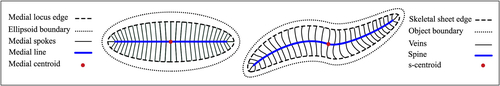Figure 4 provides an intuition about the ellipsoid’s medial locus deformation. Finally, Liu et al. (2021) generated non-crossing spokes on the skeletal sheet such that the implied boundary approximates $\partial {\Omega }_3$. The generated spokes represent a s-rep as a field of noncrossing spokes on the skeletal sheet.

Fig. 4 Skeletal sheet. Left: Ellipsoid’s medial locus. Right: s-rep skeletal sheet of a 3D-ellipsoidal.

Although we apply the method of Liu et al. (2021), we believe it is possible to improve the model fitting in many aspects such as a better boundary registration based on Jermyn et al. (2017) that we leave for future studies.

2.1.3 Local Frames

Based on the defined curves on the s-rep skeletal sheet of ellipsoidals, we can fit local frames. Let $c\subset M$ be a smooth curve in ${\mathbb{R}}^3$. We consider $\mathit{b}\in T_{\mathit{p}}(M)$ as the unit velocity vector tangent to c where $T_{\mathit{p}}(M)$ is the local tangent plane of M at $\mathit{p}\in c$ with normal n. The local frame can be defined as $(\mathit{n},\mathit{b},{\mathit{b}}^{\perp })\in SO(3)$ where ${\mathit{b}}^{\perp }=\mathit{n}\times \mathit{b}$ (see Figure 5(b)). The unit vector b chooses two opposite directions depending on the definition of the curve starting and ending points. Besides, the frame directions are noninvariant. To have a consistent invariant frame definition, we design a hierarchical structure. Then on the basis of the structure, we define consistent fitted frames in a population of GP-ds-reps.

Fig. 5 Illustration of a local frame. n is normal to tangent planes $T_{\mathit{p}}(M)$ and $T_{\mathit{p}}(M_{\Omega })$. (a) ${\mathit{s}}_1$ and ${\mathit{s}}_2$ are equal-length spokes with unit directions ${\mathit{u}}_1$ and ${\mathit{u}}_2$, and $\mathit{b}=\frac{{\mathit{u}}_1+{\mathit{u}}_2}{\left|\right|{\mathit{u}}_1+{\mathit{u}}_2\left|\right|}$ (b) c is a smooth curve on M. $-\mathit{p}{\prime }_1$ and $\mathit{p}{\prime }_2$ are the projection of ${\mathit{p}}_1$ and ${\mathit{p}}_2$ on $T_{\mathit{p}}(M)$. $\widehat{\mathit{v}}{\prime }_1=\frac{\mathit{p}-\mathit{p}{\prime }_1}{\left|\right|\mathit{p}-\mathit{p}{\prime }_1\left|\right|}$, $\widehat{\mathit{v}}{\prime }_2=\frac{\mathit{p}{\prime }_2-\mathit{p}}{\left|\right|\mathit{p}{\prime }_2-\mathit{p}\left|\right|}$, and $\mathit{b}=\frac{\widehat{\mathit{v}}{\prime }_2+\widehat{\mathit{v}}{\prime }_1}{\left|\right|\widehat{\mathit{v}}{\prime }_2+\widehat{\mathit{v}}{\prime }_1\left|\right|}$.

Consider the principal ellipsoids. Similar to Blum’s grassfire flow (Blum 1967), we can say each point on $\partial {\mathcal{E}}_2$ moves to reach the medial line ${\mathcal{E}}_1$, and then moves to reach the medial centroid ${\mathcal{E}}_0$. Thus, for each boundary point there is a path from the point to the medial centroid. In discrete format, each path can be represented by a finite set of consequent points sorted based on the distance they travel to reach the medial centroid. Imagine two consequent points on the same path. We consider the point that takes the shorter route as the parent, and the other one as the child. Therefore, like a spanning tree, each point (except medial centroid) has a parent but may have multiple children (see Figure 6(Top)). Similarly, based on the correspondence between the ${\mathcal{E}}_2$ and the skeletal sheet M, each point on the boundary (i.e., edge) of M moves on a vein to reach the spine and then moves to reach the s-centroid. Therefore, in discrete format, we define parent and child relationship on M as we defined on ${\mathcal{E}}_2$. In addition, given a frame at each skeletal point, we consider the same hierarchical structure for the frames.

Fig. 6 LP-ds-rep. Top: Hierarchical structure of the ellipsoid’s medial locus. Arrows are connections. The dot is the medial centroid. Bottom: A fitted LP-ds-rep to a hippocampus. Arrows indicate spokes, connections, and frames. The magnified image depicts a spinal frame. The dot is the s-centroid.

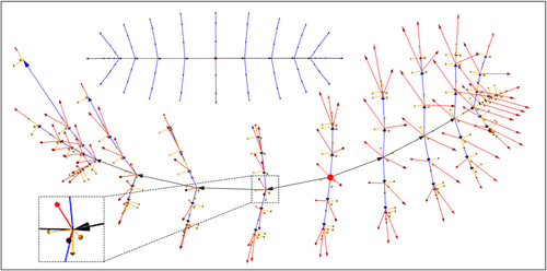
A vector that connects a frame to its parent frame is called connection. The tip of a connection is at the frame’s origin, and its tail is at the parent’s origin. Further, we assume that the s-centroid frame is its own parent without any connection to itself. We approximate the direction of b at point $\mathit{p}\in M$ based on three consecutive frames. Frames on the spine are parent of multiple children. To have a consistent frame definition first we fit frames on the spine. Except for the s-centroid frame and two critical endpoints of the spine that we will explain later, each spinal frame has a spinal parent frame and a spinal child frame. Let ${\mathit{p}}_1$ and ${\mathit{p}}_2$ be the position of the parent and the child frame of p. As illustrated in Figure 5, assume ${\mathit{v}}_1=\mathit{p}-{\mathit{p}}_1$ and ${\mathit{v}}_2={\mathit{p}}_2-\mathit{p}$ as connections. Let $\mathit{p}{\prime }_1$ and $\mathit{p}{\prime }_2$ be the projection of ${\mathit{p}}_1$ and ${\mathit{p}}_2$ on $T_{\mathit{p}}(M)$, respectively. We consider $\mathit{b}=\frac{\widehat{\mathit{v}}{\prime }_2+\widehat{\mathit{v}}{\prime }_1}{\left|\right|\widehat{\mathit{v}}{\prime }_2+\widehat{\mathit{v}}{\prime }_1\left|\right|}$ where $\widehat{\mathit{v}}{\prime }_1=\frac{\mathit{p}-\mathit{p}{\prime }_1}{\left|\right|\mathit{p}-\mathit{p}{\prime }_1\left|\right|}$, and $\widehat{\mathit{v}}{\prime }_2=\frac{\mathit{p}{\prime }_2-\mathit{p}}{\left|\right|\mathit{p}{\prime }_2-\mathit{p}\left|\right|}$. In this sense, b is a unit vector tangent to a circle (or a line) crossing $\mathit{p}-\widehat{\mathit{v}}{\prime }_1$, p, and $\mathit{p}+\widehat{\mathit{v}}{\prime }_2$.

The endpoints of the spine are critical because their frames have no children on the spine. By construction, the medial line is part of the major axis of the medial ellipse. Thus, there is a curve on the skeletal sheet correspond to the major axis that we call major curve. The major curve contains the spine and two veins. We consider the closest skeletal point (in geodesic sense) on these veins to the spine as the spine’s extension and treat the critical points as any other spinal point. The s-centroid frame has two spinal children. Let ${\mathit{p}}_1$ and ${\mathit{p}}_2$ be the position of the children. We define $\mathit{b}=\frac{\widehat{\mathit{v}}{\prime }_2-\widehat{\mathit{v}}{\prime }_1}{\left|\right|\widehat{\mathit{v}}{\prime }_2-\widehat{\mathit{v}}{\prime }_1\left|\right|}$, where $\widehat{\mathit{v}}{\prime }_1=\frac{\mathit{p}-\mathit{p}{\prime }_1}{\left|\right|\mathit{p}-\mathit{p}{\prime }_1\left|\right|}$, and $\widehat{\mathit{v}}{\prime }_2=\frac{\mathit{p}{\prime }_2-\mathit{p}}{\left|\right|\mathit{p}{\prime }_2-\mathit{p}\left|\right|}$. Since a vein frame has a parent and a child on the same vein, we consider the same definition for them as discussed for spinal frames. Note that we treat a vein frame at the intersection of a vein and the spine as a spinal frame. For the frames on the edge of the skeletal, we assume the tip of the crest spokes from Liu et al. (2021) as the position of the child frames. The same procedure is applicable for the ellipsoid’s GP-ds-rep.

Figure 6 illustrates the hierarchical structure and a fitted LP-ds-rep to a left hippocampus as we discuss in the next section.

2.1.4 LP-ds-rep

Given the fitted hierarchical frame structure introduced in the previous section, we are now in the position to define LP-ds-rep. In an LP-ds-rep, spokes and connections are measured based on their local frames, that is, their tails are located at the origin of a frame. Assume n_s , n_p , and n_c as the number of spokes, frames, and connections, respectively. Note that $n_c=n_p-1$. Let ${\mathit{u}}_i$ and ${\mathit{v}}_k$ be the ith spoke direction and kth connection direction in GCS, respectively, where $i=1,\dots ,n_s,j=1,\dots ,n_p$, and $k=1,\dots ,n_c$. Consequently, we denote ${\mathit{u}}_i^{\ast }$ and ${\mathit{v}}_k^{\ast }$ as spoke and connection directions based on their local frame, that is, we reparameterize ${\mathit{u}}_i$ and ${\mathit{v}}_k$ to ${\mathit{u}}_i^{\ast }$ and ${\mathit{v}}_k^{\ast }$, respectively. Similarly, if $F_j=({\mathit{n}}_j,{\mathit{b}}_j,{\mathit{b}}_j^{\perp })$ be the frame F_j in GCS then $F_j^{\ast }=({\mathit{n}}_j^{\ast },{\mathit{b}}_j^{\ast },{\mathit{b}}_j^{\ast \perp })$ denotes F_j based on its parent frame.

To calculate a vector direction according to a local frame, we use the spherical rotation matrix $R(\mathit{x},\mathit{y})=I_d+(\hspace{0.17em}\sin \hspace{0.17em}\alpha )(\mathit{y}{\mathit{w}}^T-\mathit{w}{\mathit{y}}^T)+(\hspace{0.17em}\cos \hspace{0.17em}\alpha -1)(\mathit{y}{\mathit{y}}^T+\mathit{w}{\mathit{w}}^T)$, where $\mathit{x},\mathit{y}\in {\mathbb{S}}^{d-1}$, $\mathit{w}=\frac{\mathit{x}-\mathit{y}({\mathit{y}}^T\mathit{x})}{\left|\right|\mathit{x-y}({\mathit{y}}^{\mathit{T}}\mathit{x})\left|\right|}$, and $\alpha ={\hspace{0.17em}\cos \hspace{0.17em}}^{-1}({\mathit{y}}^T\mathit{x})$. Therefore, $R(\mathit{x},\mathit{y})$ transfers x to y along the shortest geodesic and we have $R(\mathit{x},\mathit{y})\mathit{x}=\mathit{y}$ (Amaral, Dryden, and Wood 2007).

For example, let frame $F^{†}=(\mathit{n},\mathit{b},{\mathit{b}}^{\perp })$ be the parent of $\tilde{F}$, both in GCS. Let ${\mathit{e}}_1={(1,0,0)}^T,{\mathit{e}}_2={(0,1,0)}^T$, and ${\mathit{e}}_3={(0,0,1)}^T$ be the axes unit vectors of GCS. We align $F^{†}$ to $\tilde{I}=({\mathit{e}}_3,{\mathit{e}}_1,{\mathit{e}}_2)$ such that $R_2{R}_1{F}^{†}=\tilde{I}$, where $R_1=R(\mathit{n},{\mathit{e}}_3)$, and $R_2=R(R_1\mathit{b},{\mathit{e}}_1)$. Thus, ${\tilde{F}}^{\ast }=R_2{R}_1\tilde{F}$ represents $\tilde{F}$ in its parent coordinate system. In case we obtain $R_2{R}_1{F}^{†}=({\mathit{e}}_3,{\mathit{e}}_1,-{\mathit{e}}_2)$, we adjust the result by $R_2{R}_1\tilde{F}({\mathit{1}}_3,{\mathit{1}}_3,-{\mathit{1}}_3)$ because $R_2{R}_1{F}^{†}({\mathit{1}}_3,{\mathit{1}}_3,-{\mathit{1}}_3)=\tilde{I}$ where ${\mathit{1}}_3={(1,1,1)}^T$. Note that frame vectors are orthogonal, so after rotating n to the north pole by R₁, the shortest geodesic between b and ${\mathit{e}}_1$ would be on the equator. This preserves the direction of $R_1\mathit{n}$ while R₂ rotates $R_1\tilde{F}$.

We follow the same procedure to calculate the spokes’ and connections’ directions based on their local frames $F_j^{\ast }$. As a result, we consider a LP-ds-rep as a tuple $s^{\text{LP}}={({\mathit{u}}_i^{\ast },r_i,F_j^{\ast },{\mathit{v}}_k^{\ast },v_k)}_{i,j,k}=({\mathit{u}}_1^{\ast },\dots ,{\mathit{u}}_{n_s}^{\ast },r_1,\dots ,r_{n_s},F_1^{\ast },\dots ,$ $F_{n_p}^{\ast },{\mathit{v}}_1^{\ast },\dots ,{\mathit{v}}_{n_c}^{\ast },v_1,\dots ,v_{n_c})$, such that ${\mathit{u}}_i^{\ast }\in {\mathbb{S}}^2$ and ${\mathit{v}}_k^{\ast }\in {\mathbb{S}}^2$ are ith and kth spoke direction and connection direction relative to their local frame with lengths $r_i\in {\mathbb{R}}^{+}$ and $v_k\in {\mathbb{R}}^{+}$ respectively, and $F_j^{\ast }\in SO(3)$ is the jth frame in its parent coordinate system.

Thus, by construction, the LP-ds-rep is invariant under the act of rigid transformation. To remove the scale, we define LP-size as the geometric mean of the vectors’ lengths $\mathcal{l}=\hspace{0.17em}\exp \hspace{0.17em}(\frac{1}{n_s+n_c}({\sum }_{i=1}^{n_s}\hspace{0.17em}\ln \hspace{0.17em}(r_i)+{\sum }_{k=1}^{n_c}\hspace{0.17em}\ln \hspace{0.17em}(v_k)))$. Assume ${\rho }_i=\frac{r_i}{\mathcal{l}}$, and ${\tau }_k=\frac{v_k}{\mathcal{l}}$. A scaled LP-ds-rep can be expressed by $s^{\text{LP}}={({\mathit{u}}_i^{\ast },{\rho }_i,F_j^{\ast },{\mathit{v}}_k^{\ast },{\tau }_k)}_{i,j,k}$.

Result 1. The LP-size of a scaled LP-ds-rep is equal to one (see the proof in SUP).

Recall, for a GP-ds-rep, the GP-size is defined as the centroid size of the skeletal PDM. As we discussed in the introduction, the centroid is an extrinsic property. Thus, the centroid size might be a poor measure for the size of an object. The same discussion is also true for EDM-size where EDM-size is the geometric mean of all pairwise distances (Lele and Richtsmeier 2001, Ch.4.7.3). Intuitively, by opening or closing an arm, the arm’s volume remains the same despite its centroid size or EDM-size, that is, the closed arm has smaller centroid size and EDM-size in comparison with the open arm (see Figure 1(a)).

As Section 2.1.1 discussed, the GP-ds-rep space is ${\mathbf{S}}^{\text{GP}}={\mathbb{S}}^{3n_p-1}\times {({\mathbb{S}}^2)}^{n_s}\times {\mathbb{R}}_{+}^{n_s+1}$. In LP-ds-rep, we do not have any pre-shape space. The GOPs of an LP-ds-rep are directions and lengths of spokes, directions and lengths of connections, LP-size, and frames. Thus, the space is ${\mathbf{S}}^{\text{LP}}={({\mathbb{S}}^2)}^{n_s+n_c}\times {(SO(3))}^{n_p}\times {\mathbb{R}}_{+}^{n_s+n_c+1}$, where ${({\mathbb{S}}^2)}^{n_s+n_c}$ is the space of vectors’ directions, ${(SO(3))}^{n_p}$ is the space of the frames, and ${\mathbb{R}}_{+}^{n_s+n_c+1}$ is the space of vectors’ lengths plus LP-size. Further, we can represent an LP-ds-rep as $s^{\text{LP}}={({\mathit{u}}_i^{\ast },{\rho }_i,{\mathit{q}}_j^{\ast },{\mathit{v}}_k^{\ast },{\tau }_k)}_{i,j,k}$, where ${\mathit{q}}_j^{\ast }\in {\mathbb{S}}^3$ is the unit quaternion representation of the frame $F_j^{\ast }$ (Huynh 2009). Thus, we have ${\mathbf{S}}^{\text{LP}}={({\mathbb{S}}^2)}^{n_s+n_c}\times {({\mathbb{S}}^3)}^{n_p}\times {\mathbb{R}}_{+}^{n_s+n_c+1}$, where ${({\mathbb{S}}^3)}^{n_p}$ is the space of the frames based on their unit quaternion representations.

2.2 Euclideanization and Mean Shape

Having a population of ds-reps, suitable methods to calculate means are required in order to perform hypothesis tests on mean differences. The corresponding method should incorporate all geometrical components of the model. Both shape spaces, the GP-ds-rep space, and the LP-ds-rep space are composed of several spheres and a real space. This section will first discuss an approach to analyze the spherical parts by principal nested spheres (PNS). Afterward, approaches to produce GP-ds-rep means and LP-ds-rep means are discussed.

2.2.1 PNS

PNS (Jung, Dryden, and Marron 2012) estimates the joint probability distribution of data on d-sphere ${\mathbb{S}}^d$ by a backward view, that is, in decreasing dimension. Starting with ${\mathbb{S}}^d$, PNS fits the best lower-dimensional subsphere in each dimension. A subsphere is called great subsphere if its radius is equal to one; otherwise, it is called small subsphere. To choose between the great or small subsphere, we use the Kurtosis test from (Kim, Schulz, and Jung 2020).

PNS is designed for spherical data (particularly for small sphere distributions) to capture the curviness of circular distributions as discussed by Kim et al. (2019). PNS is similar to PCA because PCA provides observations’ coordinates called residuals as their distances from fitted (hyper)planes, while PNS residuals are the observations’ geodesic distances from the fitted subspheres. For example, the PNS residuals on ${\mathbb{S}}^2$ consist of the geodesic distances between the observations and the fitted circle and the minimal arc length between projected data on the fitted circle to the PNS mean. Basically, PNS euclideanize the data by defining a mapping from ${\mathbb{S}}^d$ to ${\mathbb{R}}^d$. In many cases, the distribution of the PNS residuals is similar to the multivariate normal distribution (see an example in SUP).

Alternatively, a simpler but faster euclideanization is to map the data on the tangent space. We transform observations to the north pole $\mathit{e}={(0,\dots ,0,1)}^T\in {\mathbb{S}}^d$ by $R({\mathit{\mu }}_F,\mathit{e})$, where ${\mathit{\mu }}_F$ is the Fréchet mean. Then, we map the transformed data to the tangent space $T_{\mathit{e}}({\mathbb{S}}^d)$ by the Log map ${\hspace{0.17em}\mathrm{Log}\hspace{0.17em}}_{\mathit{e}}(\mathit{v})=\frac{\theta }{\hspace{0.17em}\sin \hspace{0.17em}\theta }{(v_1,\dots ,v_d)}^T\in {\mathbb{R}}^d$, where $\mathit{v}={(v_1,\dots ,v_{d+1})}^T\in {\mathbb{S}}^d$, and $\theta ={\hspace{0.17em}\cos \hspace{0.17em}}^{-1}(v_{d+1})$ (Jung, Dryden, and Marron 2012; Kim, Schulz, and Jung 2020). For concentrated von Mises-Fisher distribution, the distribution of projected data to the tangent space is close to the distribution of PNS residuals (see SUP).

2.2.2 Mean GP-ds-rep

A method to produce means and shape distributions of a population of GP-ds-reps is composite PNS (CPNS) introduced by Pizer et al. (2013). The method consists of two steps. First, the two spherical parts of the GP-ds-rep shape space ${\mathbb{S}}^{3n_p-1}\times {({\mathbb{S}}^2)}^{n_s}\times {\mathbb{R}}_{+}^{n_s+1}$ are analyzed by PNS. Spokes’ lengths and scaling factor can be mapped to ${\mathbb{R}}^{n_s+1}$ with the log. Afterward, all Euclideanized variables are concatenated in addition to some scaling factors that make all variables commensurate. The covariance structure of the resulting matrix is investigated by PCA. Consequently, the mean GP-ds-rep is defined as the origin of the CPNS space. This method depends on a proper pre-alignment and is computationally expensive because PNS has to fit sequential high dimensional sub-spheres to ${\mathbb{S}}^{3n_p-1}$.

2.2.3 Mean LP-ds-rep

To formalize the estimation of LP-ds-rep mean, first we define a metric for the product space ${\mathbf{S}}^{\text{LP}}$. Assume metric spaces $({\mathbb{R}}^{+},d_l),({\mathbb{S}}^2,d_g)$ and $(SO(3),d_R)$, where $d_l(x,y)=|\hspace{0.17em}\ln \hspace{0.17em}x-\hspace{0.17em}\ln \hspace{0.17em}y|$ is the Euclidean distance of log-scaled values, $d_g(\mathit{x},\mathit{y})={\hspace{0.17em}\cos \hspace{0.17em}}^{-1}({\mathit{y}}^T\mathit{x})$ is the geodesic distance on the unit sphere (Jung, Dryden, and Marron 2012), and $d_R(F_1,F_2)=\frac{1}{\sqrt{2}}\left|\right|\hspace{0.17em}\log \hspace{0.17em}(F_1^T{F}_2)|{|}_F$ is the Riemannian distance on SO(3) where $\left|\right|.|{|}_F$ is the Frobenius norm (Moakher 2002). The distance between two scaled LP-ds-reps $s_1^{\text{LP}}={({\mathit{u}}_{1i}^{\ast },{\rho }_{1i},F_{1j}^{\ast },{\mathit{v}}_{1k}^{\ast },{\tau }_{1k})}_{i,j,k}$ and $s_2^{\text{LP}}={({\mathit{u}}_{2i}^{\ast },{\rho }_{2i},F_{2j}^{\ast },{\mathit{v}}_{2k}^{\ast },{\tau }_{2k})}_{i,j,k}$ is given by(2) $$\begin{array}{c}{d}_s(s_1^{\text{LP}},s_2^{\text{LP}})=(\sum _{i=1}^{n_s}{d}_g^2({\mathit{u}}_{1i}^{\ast },{\mathit{u}}_{2i}^{\ast })+\sum _{i=1}^{n_s}{d}_l^2({\rho }_{1i},{\rho }_{2i})\\ +\sum _{j=1}^{n_p}{d}_R^2(F_{1j}^{\ast },F_{2j}^{\ast })+\sum _{k=1}^{n_c}{d}_g^2({\mathit{v}}_{1k}^{\ast },{\mathit{v}}_{2k}^{\ast })\\ {+\sum _{k=1}^{n_c}{d}_l^2({\tau }_{1k},{\tau }_{2k}))}^{\frac{1}{2}}.\end{array}$$(2)

Remark 1.

LP-ds-rep space ${\mathbf{S}}^{\text{LP}}$ is a metric space equipped by $d_s(.)$ (see the proof in SUP).

If $s_1^{\text{LP}},\dots ,s_N^{\text{LP}}$ be a population of scaled LP-ds-reps then mean LP-ds-rep is(3) $${\overline{s}}^{\text{LP}}={\text{argmin}}_{s^{\text{LP}}\in {\mathbf{S}}^{\text{LP}}}\sum _{m=1}^N{d}_s^2(s^{\text{LP}},s_m^{\text{LP}}).$$(3)

Assume ${\overline{s}}^{\text{LP}}={({\overline{\mathit{u}}}_i^{\ast },{\overline{\rho }}_i,{\overline{F}}_j^{\ast },{\overline{\mathit{v}}}_k^{\ast },{\overline{\tau }}_k)}_{i,j,k}$ and $\forall i,j,k$ let(4) $$\begin{array}{c}{\overline{\mathit{u}}}_i^{\ast }={\text{argmin}}_{\mathit{u}\in {\mathbb{S}}^2}\sum _{m=1}^N{d}_g^2(\mathit{u},{\mathit{u}}_{im}^{\ast }),\\ {\overline{\rho }}_i={\text{argmin}}_{\rho \in {\mathbb{R}}^{+}}\sum _{m=1}^N{d}_l^2(\rho ,{\rho }_{im}),\\ {\overline{F}}_j^{\ast }={\text{argmin}}_{F\in SO(3)}\sum _{m=1}^N{d}_R^2(F,F_{jm}^{\ast }),\\ {\overline{\mathit{v}}}_k^{\ast }={\text{argmin}}_{\mathit{v}\in {\mathbb{S}}^2}\sum _{m=1}^N{d}_g^2(\mathit{v},{\mathit{v}}_{km}^{\ast }),\\ {\overline{\tau }}_k={\text{argmin}}_{\tau \in {\mathbb{R}}^{+}}\sum _{m=1}^N{d}_l^2(\tau ,{\tau }_{km}).\end{array}$$(4)

By assuming the existence of unique solutions for optimization problems (4), ${\overline{\mathit{u}}}_i^{\ast }$ and ${\overline{\mathit{v}}}_k^{\ast }$ can be estimated as the Fréchet or PNS mean of ${\left\{{\mathit{u}}_{im}^{\ast }\right\}}_{m=1}^N$ and ${\left\{{\mathit{v}}_{km}^{\ast }\right\}}_{m=1}^N$, respectively. Obviously, ${\overline{\rho }}_i$ and ${\overline{\tau }}_k$ represent the geometric means of ${\left\{{\rho }_{im}\right\}}_{m=1}^N$ and ${\left\{{\tau }_{km}\right\}}_{m=1}^N$, respectively. Further, we can calculate the mean frame ${\overline{F}}_j^{\ast }$ of ${\left\{F_{jm}^{\ast }\right\}}_{m=1}^N$ as discussed by Moakher (2002).

Result 2. If ${\overline{s}}^{\text{LP}}$ be the mean of a population of scaled LP-ds-reps, then LP-size of ${\overline{s}}^{\text{LP}}$ is equal to one (see the proof in SUP).

2.3 Converting LP-ds-rep to GP-ds-rep

Sections 2.1.3 and 2.1.4 discuss how to obtain an LP-ds-rep from a GP-ds-rep. For several reasons, for example, for visualization, we may need to reverse the procedure. For GP-ds-rep visualization, it is sufficient to draw spokes individually. To visualize an LP-ds-rep, we convert it to a GP-ds-rep. We start from $\tilde{I}$ as the s-centroid frame. Then, we reconstruct frames by finding the position and orientation of the frame’s children based on $\tilde{I}$. Afterward, we find the information of grandchildren frames based on their parents and so on.

Let frame $F^{\ast }$ be in the coordinate system of its parent $F^{†}$. To find $F^{\ast }$ based on GCS, we rotate $F^{†}$ by $R_2{R}_1$ such that $R_2{R}_1{F}^{†}=\tilde{I}$. Then ${[R_2{R}_1]}^{-1}{F}^{\ast }$ is the representation of $F^{\ast }$ in GCS. Similarly, we find the direction of connections and spokes in GCS.

Finding the mean shape of a set of objects’ boundaries without an alignment is almost impossible. But we can use LP-ds-reps to estimate the mean boundary without alignment. First, we calculate the mean LP-ds-rep. Then, we convert the mean LP-ds-rep to a GP-ds-rep. Finally, we generate the implied boundary from the GP-ds-rep as demonstrated in (Liu et al. 2021). Therefore, it is possible to approximate the mean boundary without alignment, which shows the power of LP-ds-reps.

2.4 Deformation

In statistical shape analysis generating random shapes is a matter of interest. Designing simulations based on GP-ds-reps is challenging as we usually need to identify a local frame to bend or twist the object locally. It turned out that LP-ds-reps support naturally skeletal deformations. We can stretch, shrink, bend, and twist the skeletal by manipulating the frames’ orientations and vectors’ lengths. Then, we convert the LP-ds-rep to a GP-ds-rep to generate the boundary. Consequently, we can add variation to a set of deformed LP-ds-reps’ GOPs to simulate random ds-reps. Figure 7 shows a deformed hippocampus including bending and twisting. The deformation is based on the rotation of spinal frames.

Fig. 7 Skeletal deformation by LP-ds-rep. Left: A ds-rep with its implied boundary in two angles. Middle: Shape bending by spinal frame rotation about n and ${\mathit{b}}^{\perp }$ axes. Right: Shape twisting by spinal frames rotation about b axis.

3 Hypothesis Testing

For LP-ds-rep hypothesis testing, we consider frames as unit quaternions (i.e., $s^{\text{LP}}={({\mathit{u}}_i^{\ast },{\rho }_i,{\mathit{q}}_j^{\ast },{\mathit{v}}_k^{\ast },{\tau }_k)}_{i,j,k}$). In this sense, euclideanization of the frames based on their unit quaternion representation is the same as other spherical data as we discussed in Section 2.2.

Let $A={\left\{s_A{}_m\right\}}_{m=1}^{N_1}$ and $B={\left\{s_B{}_m\right\}}_{m=1}^{N_2}$ be two groups of either GP-ds-reps or LP-ds-reps of sizes N₁ and N₂. Let $n_{\text{GOP}}$ be the total number of GOPs. To test GOPs’ mean difference, we design $n_{\text{GOP}}$ partial tests. Let ${\overline{s}}_A(n)$ and ${\overline{s}}_B(n)$ be the observed sample mean of the nth GOP from A and B respectively. The partial test is $H_{0n}:{\overline{s}}_A(n)={\overline{s}}_B(n)$ versus $H_{1n}:{\overline{s}}_A(n)\ne {\overline{s}}_B(n)$. Note that for GP-ds-rep, LP-ds-rep, and EDM of the skeletal PDM, $n_{\text{GOP}}$ is $(n_p+2n_s+1),(2n_s+n_p+2n_c+1)$, and $(\frac{(n_p-1)n_p}{2}+1)$, respectively.

To test mean differences, we adapted a nonparametric permutation test with minimal assumptions similar to Styner’s approach (Styner et al. 2006). For the univariate data, that is, vectors’ lengths and shapes’ sizes, the test statistic is t-statistic $T=\frac{\overline{x}-\overline{y}}{S_p\sqrt{\frac{1}{N_1}+\frac{1}{N_2}}}$ where S_p is the pooled standard deviation. For the multivariate data, that is, euclideanized directions and GP-ds-rep skeletal positions, the test statistic is Hotelling’s T² metric $T^2={(\overline{\mathit{x}}-\overline{\mathit{y}})}^T{\widehat{\Sigma }}^{-1}(\overline{\mathit{x}}-\overline{\mathit{y}})$, where $\widehat{\Sigma }$ is an unbiased estimate of common covariance matrix (Martin and Maes 1979, ch.3). Given the pooled group {A, B}, the permutation method randomly partitions B times the pooled group into two paired groups of sizes N₁ and N₂ without replacement, where usually we consider $B\ge {10}^4$. Afterward, it measures the test statistic between the paired groups. The empirical p-value for the nth GOP is ${\eta }_n=\frac{1+{\sum }_{h=1}^B{\chi }_E(|T_{nh}|\ge T_{no})}{B+1}$, where T_no is the nth observed test statistics, T_nh is the hth permutation test statistic, and χ_E is the indicator function, that is, ${\chi }_E(\phi )=1$ if $\phi$ is true, otherwise ${\chi }_E(\phi )=0$. Note that if we have normally distributed data, it is reasonable to apply Hotelling’s T² test (with normality assumption) instead of the permutation test as it is much faster.

In order to account for the problem of multiple hypothesis testing, one could use the method of Bonferroni (1936). Bonferroni’s method tests each hypothesis at level $\alpha /n_{\text{GOP}}$ and guarantees the probability of at least one Type I error $P(v\ge 1)$ be less than the significance level $\alpha$. Since the method is highly conservative we prefer to use Benjamini and Hochberg (1995) (BH) method as a more moderate approach.

4 Evaluation

4.1 Data

To test our method, we study the hippocampal difference between early Parkinson’s disease (PD) and CG at baseline. Data are provided by ParkWest (http://parkvest.no), in cooperation with Stavanger University Hospital (https://helse-stavanger.no). At the baseline, we have 182 magnetic resonance images for PD and 108 for CG with corresponding segmentation of hippocampi. As described in Section 2, GP-ds-reps are fitted to left hippocampi by SlicerSALT toolkit (http://salt.slicer.org) and reparameterize into LP-ds-reps. For the model fitting, we used GP-ds-reps with 122 spokes consisting of 51 up, 51 down, and 20 crest spokes. As up and down spokes share the same tail positions, we have in total 71 tail positions. The generated LP-ds-reps have 122 spokes, 71 local frames, and 70 connections. Before analyzing the ParkWest data, we first study our method based on simulations.

4.2 Simulation

For the simulation study, we select a LP-ds-rep close to the mean LP-ds-rep of CG as a template. Based on the template, we generate two groups of LP-ds-reps each of size 150 with different amount of tail bending, that is, bending in a local region. Such bending was observed, for example, in (Pizer et al. 2003) between schizophrenics and controls. Let ${\mathcal{M}}_d(\mathit{\mu },\kappa )$ denotes von Mises-Fisher distribution with mean $\mathit{\mu }$ and concentration parameter κ on ${\mathbb{S}}^{d-1}$ (Dhillon and Sra 2003). For the special case d = 2 we assume the distribution in radian, that is, $\theta ,\mu \in [0,2\pi )$ if $\theta \sim {\mathcal{M}}_2(\mu ,\kappa )$. Given a random rotation angle of bending $\theta \sim {\mathcal{M}}_2(\mu =0,\kappa =100)$ for the first group and $\theta \sim {\mathcal{M}}_2(\mu =\frac{-\pi }{15},\kappa =100)$ for the second group, we simulate the orientation of three spinal frames by successively rotating them about their ${\mathit{b}}^{\perp }$-axis with ${[R_2{R}_1]}^{-1}R({\mathit{e}}_3,{(\hspace{0.17em}\cos \hspace{0.17em}\theta ,0,\hspace{0.17em}\sin \hspace{0.17em}\theta )}^T)\tilde{I}$. This means the tails in the second group are successively bent on average ${12}^{°}$ downward for three consecutive spinal frames. Chosen frames are the closest ones on the hippocampus tail to the s-centroid. Thus, in total, we have a slight downward bending about ${36}^{°}$ at the hippocampus tail. Finally, by preserving frame orthogonality, we add noise to all directions by ${\mathcal{M}}_3(\mathit{\mu },\kappa )$, where κ for frames’ vectors, spokes, and connections is equal to 600, 250, and 5000, respectively. 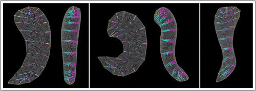Further additional noise is added to vectors’ lengths by the truncated normal distribution $\psi (\mu ,\sigma ,a>0,b<\infty )$ where μ is the vector length of the template, and parameters σ, a, and b are heuristically chosen. As a result, we have two groups of random LP-ds-reps, which are approximately similar in most of their GOPs but only different in the orientation of three frames. Figure 8 illustrates twenty samples of each group. Note that LP-ds-reps are not aligned, but since we reconstruct them from the s-centroid frame, shapes have Bookstein’s alignment (Dryden and Mardia 2016, Ch.2) because the s-centroid frames are perfectly aligned.

Fig. 8 Simulation. Left: Two groups of simulated ds-reps. Middle: Overlaid mean LP-ds-reps. Right: Illustration of local frames. Bold frames are statistically significant.

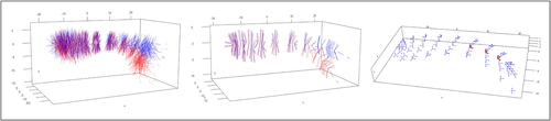
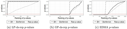
As depicted in Figure 8(Right), hypothesis test on LP-ds-rep from Section 3 correctly detects significant frame directions and label almost all other GOPs as statistically nonsignificant given a significance level $\alpha =0.05$. On the contrary, as depicted in Figure 9, the test on GP-ds-reps indicates a large number of false positives, that is, almost all of the positions and directions are statistically significant. Also, from EDMA on the skeletal PDM we can see that about half of the distances are significant. This example confirms our observation from Figure 1 in Section 1, and highlights the fact that noninvariant GP-ds-rep analysis is biased and invariant EDMA could be misleading. The power of LP-ds-rep is further highlighted by additional simulation examples provided in SUP.

Fig. 9 Sorted raw and adjusted p-values. The horizontal line indicates significance level $\alpha =0.05$.

4.3 Real Data Analysis

The Parkinson dataset described in Section 4.1 was studied earlier by (Apostolova et al. 2012) based on radial distance analysis and parallel slicing and showed some regional atrophy. Since shape correspondence in noninvariant parallel slicing method is controversial, we attempt to reanalyze data by utilizing LP-ds-reps.

First let us compare the shape sizes from Table 1. The volume measurement confirms the LP-size is more compatible with the object volume because both, the mean object volume and the LP-size of CG, are greater than PD. In opposite the mean GP-size and EDM-size of CG are smaller than PD. Also, tests on shape size indicate significant difference in LP-size.

Table 1 T-test on shape size.

	Mean CG	Mean PD	SD CG	SD PD	p-value
Object volume (mm^3)	3352.23	3271.44	563.39	616.68	0.26
LP-size	2.37	2.33	0.17	0.18	0.04
GP-size of spokes’ tips	161.05	162.51	8.97	8.62	0.17
EDM-size of skeletal PDM	12.66	12.76	0.83	0.84	0.36

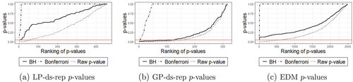
Figure 10 illustrates significant LP-ds-rep and GP-ds-rep GOPs before and after BH adjustment. In LP-ds-rep, all the spokes directions are insignificant. In contrast, about 40% of GP-ds-rep spokes’ directions are significant. Also, in LP-ds-rep, there are a few significant connection and frame directions after the adjustment. Based on the LP-ds-rep analysis, it seems the main difference comes from connections’ lengths on the spine. Figure 11 shows sorted p-values before and after adjustment of the applied methods. Based on Bonferroni adjustment, PD and CG are similar because almost all adjusted p-values are greater than 0.05. Based on BH adjustment, all GOPs in EDMA are not significant but about 30% of them are significant before BH adjustment. The reason is the sensitivity of BH to the number of tests, that is, by increasing the number of tests, BH becomes conservative. In GP-ds-rep half of the GOPs are significant even after the BH adjustment. In contrast, LP-ds-rep shows a small portion of significant GOPs before and after the adjustment. In addition, we analyzed the shapes without scaling to show the sensitivity of GP-ds-rep to the scaling and the superiority of LP-ds-rep compared to GP-ds-rep and EDMA. Detailed results are available in SUP.

Fig. 10 ds-rep significant GOPs. Bold indicate significant GOPs. FDR = 0.05 for BH adjustment.

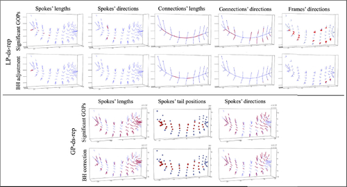
Fig. 11 Test on real data. Sorted raw and adjusted p-values. The horizontal line indicates significance level 0.05.

5 Conclusion

Generally, it is common to detect locational dissimilarity between two groups of objects based on the alignment. As discussed, noninvariant (i.e., alignment-dependent) methods such as GP-ds-rep analysis could be highly biased, and invariant methods based on extrinsic object properties like EDMA could be misleading. Thus, we propose an invariant shape representation called LP-ds-rep by putting a partial order on the skeletal positions of a GP-ds-rep and constructing local frames at each skeletal position. Such partial order exists on any tree structure, by considering the flow away from a chosen basepoint. Therefore, the proposed idea is not limited to ellipsoidal objects, neither to skeletal models, as long as a tree structure can be established for a shape model that ensures good correspondence between objects. Further, we compared LP-ds-rep analysis with GP-ds-rep analysis and EDMA to show the power and the advantages of LP-ds-reps. For comparison, we applied simulation and real data analysis. The simulation confirmed that even if two populations of ds-reps differ only in a small local region, the hypothesis tests based on GP-ds-reps and EDMs result in a large number of significant GOPs while the tests based on LP-ds-reps indeed detect the true underlying differences. We studied left hippocampi of PD versus CG for real data analysis. Although hypothesis tests on GP-ds-reps and EDMs indicated many significant GOPs, tests on LP-ds-reps showed only a few, which seems medically more reasonable. We concluded that PD and CG groups are very similar, but the main difference comes from the spine length.

Acknowledgments

Special thanks to Profs. Stephen M. Pizer (UNC), Steve Maron (UNC), James Damon (UNC), and Jan Terje Kvaløy (UiS) for insightful discussions and inspiration for this work. We are indebted to Prof. Guido Alves (UiS) for providing ParkWest data. We also thank Zhiyuan Liu (UNC) for the model fitting toolbox.

Supplementary Materials

Supplementary: SUP materials referenced in this work are available as a pdf. (pdf)

R-code: In Supplementary.zip, simulation codes and files are placed. (zip)

Additional information

Funding

This research is funded by the Department of Mathematics and Physics of the University of Stavanger (UiS).

Notes

1 The required energy to deform one object to the other one is negligible, for example, see Sorkine (2006).

2 Tube refers to a 3D object made by a sweeping disk such that its medial locus is a smooth curve.

3 Slab refers to a 3D object such that its medial locus is a sheet.

4 See Van Kaick et al. (2011) for a comprehensive discussion about meaningful correspondence.

References

- Amaral, G. A., Dryden, I., and Wood, A. T. A. (2007), “Pivotal Bootstrap Methods for k-Sample Problems in Directional Statistics and Shape Analysis,” Journal of the American Statistical Association, 102, 695–707. DOI: 10.1198/016214506000001400.
- Apostolova, L., Alves, G., Hwang, K. S., Babakchanian, S., Bronnick, K. S., Larsen, J. P., Thompson, P. M., Chou, Y. Y., Tysnes, O. B., and Vefring, H. K. (2012), “Hippocampal and Ventricular Changes in Parkinson’s Disease Mild Cognitive Impairment,” Neurobiology of Aging, 33, 2113–2124. DOI: 10.1016/j.neurobiolaging.2011.06.014.
- Benjamini, Y., and Hochberg, Y. (1995), “Controlling the False Discovery Rate: A Practical and Powerful Approach to Multiple Testing,” Journal of the Royal Statistical Society, Series B, 57, 289–300. DOI: 10.1111/j.2517-6161.1995.tb02031.x.
- Berger, J. (1985), Statistical Decision Theory and Bayesian Analysis. Springer Series in Statistics, Berlin: Springer. https://books.google.no/books?id=oY/_x7dE15/_AC.
- Blum, H. (1967), “A Transformation for Extracting New Descriptors of Shape,” Symp. on Models for the Perception of Speech and Visual Form. Cambridge, MA: MIT Press.
- Bonferroni, C. (1936), “Teoria Statistica delle Classi e Calcolo delle Probabilita,” Pubblicazioni del R Istituto Superiore di Scienze Economiche e Commericiali di Firenze, 8, 3–62.
- Cartan, E. (1937), La théorie des groupes finis et continus et la géométrie différentielle: traitées par la méthode du repère mobile/leçons professées la Sorbonne par Elie Cartan,…; rédigées par Jean Leray,…Cahiers scientifiques, Paris: Gauthier-Villars.
- Damon, J. (2008), “Swept Regions and Surfaces: Modeling and Volumetric Properties,” Theoretical Computer Science, 392, 66–91. DOI: 10.1016/j.tcs.2007.10.004.
- Damon, J., and Marron, J. (2014), “Backwards Principal Component Analysis and Principal Nested Relations,” Journal of Mathematical Imaging and Vision, 50, 107–114. DOI: 10.1007/s10851-013-0463-2.
- Dhillon, I. S., and Sra, S. (2003), “Modeling Data Using Directional Distributions,” Technical Report, Citeseer.
- Dryden, I., and Mardia, K. (2016), Statistical Shape Analysis: With Applications in R. (Vol. 995). Chichester: John Wiley & Sons.
- Fletcher, P. T., Lu, C., and Joshi, S. (2003), “Statistics of Shape via Principal Geodesic Analysis on Lie Groups,” In Proceedings, 2003 IEEE Computer Society Conference on Computer Vision and Pattern Recognition, 2003. IEEE, vol 1, pp. I–I.
- Fletcher, P. T., Lu, C., Pizer, S. M., and Joshi, S. (2004), “Principal Geodesic Analysis for the Study of Nonlinear Statistics of Shape,” IEEE Transactions on Medical Imaging, 23, 995–1005. DOI: 10.1109/TMI.2004.831793.
- Gamble, J., and Heo, G. (2010), “Exploring Uses of Persistent Homology for Statistical Analysis of Landmark-Based Shape Data,” Journal of Multivariate Analysis, 101, 2184–2199. DOI: 10.1016/j.jmva.2010.04.016.
- Huynh, D. Q. (2009), “Metrics for 3D Rotations: Comparison and Analysis,” Journal of Mathematical Imaging and Vision, 35, 155–164. DOI: 10.1007/s10851-009-0161-2.
- Jermyn, I. H., Kurtek, S., Laga, H., Srivastava, A. (2017), “Elastic Shape Analysis of Three-Dimensional Objects,” Synthesis Lectures on Computer Vision, 12, 1–185.
- Jung, S., Dryden, I. L., and Marron, J. (2012), “Analysis of Principal Nested Spheres,” Biometrika, 99, 551–568. DOI: 10.1093/biomet/ass022.
- Kendall, D. G. (1977), “The Diffusion of Shape,” Advances in Applied Probability, 9, 428–430. DOI: 10.2307/1426091.
- Kim, B., Huckemann, S., Schulz, J., and Jung, S. (2019), “Small-Sphere Distributions for Directional Data with Application to Medical Imaging,” Scandinavian Journal of Statistics, 46, 1047–1071. DOI: 10.1111/sjos.12381.
- Kim, B., Schulz, J., and Jung, S. (2020), “Kurtosis Test of Modality for Rotationally Symmetric Distributions on Hyperspheres,” Journal of Multivariate Analysis, 178, 104603. DOI: 10.1016/j.jmva.2020.104603.
- Laga, H., Guo, Y., Tabia, H., Fisher, R., and Bennamoun, M. (2018), 3D Shape Analysis: Fundamentals, Theory, and Applications. Hoboken, NJ: Wiley. https://books.google.no/books?id=ds16DwAAQBAJ.
- Lele, S. R., and Richtsmeier, J. T. (1991), “Euclidean Distance Matrix Analysis: A Coordinate-Free Approach for Comparing Biological Shapes Using Landmark Data,” American Journal of Physical Anthropology, 86, 415–427. DOI: 10.1002/ajpa.1330860307.
- Lele, S. R., and Richtsmeier, J. T. (2001), An Invariant Approach to Statistical Analysis of Shapes. Boca Raton, FL: Chapman and Hall/CRC.
- Liu, Z., Hong, J., Vicory, J., Damon, J. N., and Pizer, S. M. (2021), “Fitting Unbranching Skeletal Structures to Objects,” Medical Image Analysis, 70, 102020. DOI: 10.1016/j.media.2021.102020.
- Martin, N., and H. Maes. (1979). Multivariate analysis. London, UK: Academic Press.
- Moakher, M. (2002), “Means and Averaging in the Group of Rotations,” SIAM Journal on Matrix Analysis and Applications, 24, 1–16 DOI: 10.1137/S0895479801383877.
- Pizer, S. M., Fritsch, D. S., Yushkevich, P. A., Johnson, V. E., and Chaney, E. L. (1999), “Segmentation, Registration, and Measurement of Shape Variation via Image Object Shape,” IEEE Transactions on Medical Imaging, 18, 851–865. DOI: 10.1109/42.811263.
- Pizer, S. M., Fletcher, P. T., Thall, A., Styner, M., Gerig, G., and Joshi, S. (2003), “Object Models in Multiscale Intrinsic Coordinates via m-Reps,” Image and Vision Computing, 21, 5–15. DOI: 10.1016/S0262-8856(02)00130-0.
- Pizer, S. M., Jung, S., Goswami, D., Vicory, J., Zhao, X., Chaudhuri, R., Damon, J. N., Huckemann, S., and Marron, J. (2013), “Nested Sphere Statistics of Skeletal Models,” in Innovations for Shape Analysis, Berlin, Heidelberg: Springer, pp. 93–115.
- Rustamov, R. M., Lipman, Y., and Funkhouser, T. (2009), “Interior Distance Using Barycentric Coordinates,” in Computer Graphics Forum, Oxford, UK: Blackwell Publishing Ltd, Vol. 28, pp. 1279–1288. DOI: 10.1111/j.1467-8659.2009.01505.x.
- Schulz, J. (2013), “Statistical Analysis of Medical Shapes and Directional Data,” PhD thesis, UiT Norges arktiske universitet.
- Siddiqi, K., and Pizer, S. (2008), Medial Representations: Mathematics, Algorithms and Applications. Computational Imaging and Vision, Dordrecht, Netherlands: Springer Netherlands
- Sorkine, O. (2006), “Differential Representations for Mesh Processing,” in Computer Graphics Forum, Oxford, UK: Blackwell Publishing Ltd, vol. 25, pp. 789–807. DOI: 10.1111/j.1467-8659.2006.00999.x.
- Srivastava, A. and Klassen, E. (2016), Functional and Shape Data Analysis. Springer. Series in Statistics, New York: Springer, https://books.google.no/books?id=0cMwDQAAQBAJ.
- Styner, M., Oguz, I., Xu, S., Brechbühler, C., Pantazis, D., Levitt, J. J., Shenton, M. E., and Gerig, G. (2006), “Framework for the Statistical Shape Analysis of Brain Structures Using spharm-pdm.” The Insight Journal, 242–250. DOI: 10.54294/owxzil.
- Tabia, H., and Laga, H. (2015), “Covariance-Based Descriptors for Efficient 3D Shape Matching, Retrieval, and Classification,” IEEE Transactions on Multimedia, 17, 1591–1603. DOI: 10.1109/TMM.2015.2457676.
- Turner, K., Mukherjee, S., and Boyer, D. M. (2014), “Persistent Homology Transform for Modeling Shapes and Surfaces,” Information and Inference: A Journal of the IMA, 3, 310–344. DOI: 10.1093/imaiai/iau011.
- Van Kaick, O., Zhang, H., Hamarneh, G., and Cohen-Or, D. (2011), “A Survey on Shape Correspondence,” in Computer Graphics Forum, Oxford, UK: Blackwell Publishing Ltd, vol. 30, pp. 1681–1707. DOI: 10.1111/j.1467-8659.2011.01884.x.