EM Algorithm for the Estimation of the RETAS Model

Abstract

The Renewal Epidemic-Type Aftershock Sequence (RETAS) model is a recently proposed point process model that can fit event sequences such as earthquakes better than preexisting models. Evaluating the log-likelihood function and directly maximizing it has been shown to be a viable approach to obtain the maximum likelihood estimator (MLE) of the RETAS model. However, the direct likelihood maximization suffers from numerical issues such as premature termination of parameter searching and sensitivity to the initial value. In this work, we propose to use the Expectation-Maximization (EM) algorithm as a numerically more stable alternative to obtain the MLE of the RETAS model. We propose two choices of the latent variables, leading to two variants of the EM algorithm. As well as deriving the conditional distribution of the latent variables given the observed data required in the E-step of each EM-cycle, we propose an approximation approach to speed up the E-step. The resulting approximate EM algorithms can obtain the MLE much faster without compromising on the accuracy of the solution. These newly developed EM algorithms are shown to perform well in simulation studies and are applied to an Italian earthquake catalog. Supplementary materials for this article are available online.

KEYWORDS:

• MLE
• Point process
• Renewal process
• Seismology
• Self-exciting

1 Introduction

The self-exciting point process of Hawkes (1971) has an intensity process which consists of a long-term constant background rate plus short-term self-excitement effects due to the points (events) in its history. By the cluster process representation of the Hawkes process (Hawkes and Oakes 1974), each event of the process can be interpreted as either an immigrant or an offspring, where the immigrants arrive according to a homogeneous Poisson process and each immigrant potentially generates offspring according to a common inhomogeneous Poisson process, and each offspring can then trigger additional offspring of their own according to the same inhomogeneous Poisson process.

Since the introduction of the Hawkes (1971) process, several model innovations have been proposed in the literature with widespread use in many application domains. The RHawkes process (Wheatley, Filimonov, and Sornette 2016) is one such innovation that replaces the constant background rate in the intensity of the Hawkes process with a time-dependent function that resets on the arrival of each immigrant and then evolves according to a fixed function of time. This is equivalent to replacing the homogeneous Poisson immigrant arrival process with a renewal process where the waiting times between successive events have the fixed function of time as their common hazard rate function. Similar to the Poisson process, the renewal process has iid inter-event waiting times, but it differs in that a general waiting time distribution can be used instead of the exponential distribution. With this generalization of the immigrant arrival process it becomes possible to model diverse temporal clustering characteristics such as those with roughly evenly distributed clusters, and those with occasional large gaps between events.

The ETAS model (Ogata 1988) is an extended version of the Hawkes self-exciting point process where the excitation effect of an event is allowed to depend on the mark associated with the event (e.g., the magnitude of an earthquake). The ETAS model also has a spatiotemporal extension (Ogata 1998) which has been influential in various fields, such as seismology (Ogata and Zhuang 2006; Guo, Zhuang, and Zhou 2015), criminology (Mohler et al. 2011; Lewis and Mohler 2011; Zhuang and Mateu 2019) and epidemiology (Meyer, Elias, and Höhle 2012). Specifically, in seismology, the immigrant events can be interpreted as main-shocks and the offspring events as aftershocks. In the same spirit of the RHawkes process being a modification to the Hawkes process, the RETAS model (Stindl and Chen 2022, 2023) is a modification to the ETAS model, where the main-shock arrival times follow a renewal process rather than a homogeneous Poisson process. The RETAS model might be considered a special case of the general modulated renewal process proposed by Lin and Fine (2009) with the backward recurrence time V_t defined as the time lapsed from the previous immigrant (mainshock), although an important difference to note is that the backward recurrence time is unobserved in the RETAS model, while it is assumed part of the data in Lin and Fine (2009).

Likelihood based inferences such as maximum likelihood estimation are typically straightforward to implement for self-exciting point processes. However, this is not the case for the RETAS model since the conditional intensity process depends on the unobserved index of the most recent immigrant, and the standard formula for point processes likelihood cannot be used directly to calculate its likelihood. Instead, Stindl and Chen (2022) proposed a recursive algorithm to calculate the likelihood and demonstrated that the MLE can be obtained by numerically maximizing the likelihood. However, direct optimization of the likelihood might be numerically unstable or computationally costly, as noted by Veen and Schoenberg (2008) for the ETAS model. These issues can be mitigated using the Expectation-Maximization (EM) algorithm of Dempster, Laird, and Rubin (1977), as shown in Marsan and Lengliné (2008), Veen and Schoenberg (2008), and Lewis and Mohler (2011).

Rather than maximizing the log-likelihood directly, the EM algorithm iteratively maximizes the conditional expectation of the complete data log-likelihood given the observed data and the current estimate of the parameter before setting the maximizer as the updated parameter. This achieves the same objective of maximizing the observed data log-likelihood while mitigating some of the numerical instabilities of direct maximization caused by multi-modality and flat surfaces. Although the EM algorithm does not completely resolve the issues associated with converging to a local maximum, its numerical performance tends to be more stable. The estimation of the ETAS and RETAS model can be posed in the EM framework where the observed data consists of the occurrence times of the earthquakes and the associated marks such as the epicenters and magnitudes and the branching structure consisting of the indicators for main-shocks and triggered aftershocks serves as the set of unobserved latent variables.

Wheatley, Filimonov, and Sornette (2016) proposed an EM algorithm in the spirit of Dempster, Laird, and Rubin (1977) for the RHawkes process. This is a promising endeavor due to its success for the Hawkes and ETAS models. The approach by Wheatley, Filimonov, and Sornette (2016) modified the EM algorithms of Veen and Schoenberg (2008), Marsan and Lengliné (2008), and Lewis and Mohler (2011) to allow for a renewal immigrant arrival process. They also introduced a version of the EM algorithm with a reduced set of latent variables that only included a binary variable for immigrants rather than the complete branching structure. However, in their implementation of the EM algorithm, the expectation in the E-step is calculated with respect to a conditional distribution that conditions on a varying subset of the observed data rather than the entire set. For the classical ETAS model this did not cause concern because of the conditional independence of past immigrant/offspring indicators and future events times given past event times. However, this is not the case for the RETAS model and the objective of this article is to amend the aforementioned EM algorithms of Wheatley, Filimonov, and Sornette (2016) by conditioning on the whole set of observed data in implementing the E-step.

Hence, we propose a recursive algorithm to calculate the conditional probabilities needed in the E-step. We first calculate the filtered most recent immigrant probabilities which only condition on a subset of the observed data. Then, we smooth the filtered probabilities to obtain the smoothed most recent immigrant probabilities which condition on the entire observed data. These probabilities facilitate the calculation of the smoothed branching structure probabilities such as the immigrant and parent probabilities. The M-step can then be implemented as in Wheatley, Filimonov, and Sornette (2016). We also provide a strategy to reduce the computational time of the EM algorithm that follows the procedure discussed in Stindl and Chen (2021) to accelerate the calculation of the log-likelihood for the RHawkes process. This approach truncates the distribution of the most recent immigrant and restricts the longevity of the self-excitation effects.

The remainder of this article is devoted to the following. Section 2 describes the RETAS model and the log-likelihood evaluation algorithm. Section 3 presents the whole data EM algorithm for the RETAS model. Section 4 introduces an approximation in the E-step to accelerate the EM algorithms. Section 5 provides numerical evidence that the EM algorithms converge to the MLE using simulated data, and a comparison to direct log-likelihood maximization to obtain the MLE is also presented. The article concludes with a case study of an Italian earthquake catalog in Section 6.

2 RETAS Model

Let the occurrence time be denoted by τ_i with ${\tau }_{i-1}<{\tau }_i$ and the associated mark be denoted by m_i. The cumulative number of events up to and including time t is given by the counting process $\left\{N(t),t\ge 0\right\}$ with $N(t)={\sum }_{i=1}^{n}1\{{\tau }_i\le t\}$, where $1\{·\}$ is the indicator function. Suppose that the marked point process is realized over the interval $[0,T]$ with T denoting the censoring time, $n=N(T)$ being the total number of events, ${\tau }_{1:n}=({\tau }_1,\dots ,{\tau }_n)$ containing all the observed event times and $m_{1:n}=(m_1,\dots ,m_n)$ containing all the corresponding event marks. The conditional intensity process of the RETAS model describes the instantaneous arrival rate of events at time t which depends on all past event occurrence times and marks. We define ${\mathcal{H}}_{t-}=\left\{N(t-),({\tau }_i,m_i) : i=1,2,\dots ,N(t-)\right\}$ to be the internal history of the process just prior to time t. We also extend the definition of internal history to include the index of the most recent immigrant $I(t)=\max \left\{i ; {\tau }_i<t,B_i=0\right\}$ where B_i = 0 indicates that the ith event is an immigrant, and define ${\tilde{\mathcal{H}}}_{t-}={\mathcal{H}}_{t-}\cup \{I(s),0\le s\le t\}$ to be the extended history.

The conditional intensity process for the RETAS model with respect to the extended history ${\tilde{\mathcal{H}}}_{t-}$ is a superposition of a time-varying background rate that renews at immigrant arrivals and a self-exciting term consisting of cumulative excitation effects due to past events (1) $$\lambda (t|{\tilde{\mathcal{H}}}_{t-})=\mu (t-{\tau }_{I(t)})+\sum _{j=1}^{N(t-)}\psi (t-{\tau }_j,m_j),$$(1) see (1) in Stindl and Chen (2019). The function $\mu :{\mathbb{R}}^{+}\to {\mathbb{R}}^{+}$ is a deterministic hazard rate function of the renewal distribution for the waiting time between successive immigrants. The excitation function $\psi (t-{\tau }_j,m_j)$ describes the intensity of an inhomogenous Poisson process for an offspring originating at the occurrence time τ_j with mark m_j. Herein, we assume that the excitation function is separable, $\psi (t,m)=g(t)k(m)$ and comprises of a temporal response function $g:{\mathbb{R}}^{+}\to {\mathbb{R}}^{+}$ and a boost function $k:\mathcal{M}\to {\mathbb{R}}^{+}$ where $\mathcal{M}$ represents the mark space. If g is a density function such that ${\int }_0^{\infty }g(t)\mathrm{d}t=1$ then the boost function k determines the expected number of offspring due to a single event (with mark m) while the temporal response function describes the arrival time of the offspring event relative to its parent.

This model generalization introduces intricate dependencies between the clusters where a cluster consists of an immigrant and its multi-generational sequence of offspring. This additional flexibility comes at a cost as the classical formula of the observed data log-likelihood (see e.g., Daley and Vere-Jones 2003) given by (2) $$\mathcal{l}(\theta )=\sum _{i=1}^{N(T)}\hspace{0.17em}\log \hspace{0.17em}\lambda ({\tau }_i|{\mathcal{H}}_{{\tau }_i-})-{\int }_0^T\lambda (s|{\mathcal{H}}_{s-})\mathrm{d}s,$$(2) is not convenient for likelihood evaluation, since for the RETAS model, knowledge of the most recent immigrant event is required to define the renewal times. However, Chen and Stindl (2018) bypassed the formula in (2) and developed an algorithm to evaluate the likelihood recursively for the RHawkes process by conditioning on the most recent immigrant. The algorithm provides an alternate but equivalent expression to calculate the likelihood in (2) without resorting to first calculating the intensity process with respect to the internal history ${\mathcal{H}}_t$, whose form is rather complex.

For ease of reference, we reproduce the log-likelihood evaluation algorithm for the RETAS model (adapted from Stindl and Chen 2021). Let the filtered probabilities for the index of the most recent immigrant be denoted by $p_{ij}=\mathbb{P}(I({\tau }_i)=j|{\tau }_{1:i-1},m_{1:i-1})$ for $j=1,\dots ,i-1$; $i=2,\dots ,n+1$. Define $$\begin{array}{c}\varphi (t)=\sum _{j:{\tau }_j<t}g(t-{\tau }_j)k(m_j),\\ \Phi (T)=\sum _{j:{\tau }_j<T}k(m_j){\int }_{{\tau }_j}^{T}g(t-{\tau }_j) \mathrm{d}t,\end{array}$$and for $j=1,\dots ,i-1$; $i=2,\dots ,n+1$ $$d_{ij}=\left(\mu ({\tau }_i-{\tau }_j)+\varphi ({\tau }_i)\right)S_{ij},\hspace{1em}{S}_{ij}=e^{-{\int }_{{\tau }_{i-1}}^{{\tau }_i}\mu (t-{\tau }_j)\mathrm{d}t},$$

where ${\tau }_{n+1}:=T$. Further define $d_1=\mu ({\tau }_1)e^{-{\int }_0^{{\tau }_1}\mu (t)\mathrm{d}t}$. The log-likelihood of the RETAS model is given by (3) $$\mathcal{l}(\theta )=\hspace{0.17em}\log \hspace{0.17em}{d}_1+\sum _{i=2}^n\hspace{0.17em}\log \hspace{0.17em}\left(\sum _{j=1}^{i-1}{p}_{ij} d_{ij}\right)+\hspace{0.17em}\log \hspace{0.17em}\left(\sum _{j=1}^n{p}_{n+1,j}{S}_{n+1,j}\right)+\Phi (T),$$(3) and the p_ij’s are calculated recursively by (4) $$p_{ij}=\{\begin{array}{cc}\frac{p_{i-1,j}\varphi ({\tau }_{i-1})S_{i-1,j}}{\sum _{k=1}^{i-2}{p}_{i-1,k}{d}_{i-1,k}},\hfill & j=1,\dots ,i-2\hfill \\ 1-\sum _{k=1}^{i-2}{p}_{ik},\hfill & j=i-1\hfill \end{array},\hspace{1em}i\ge 3,$$(4) with the initial condition $p_{21}=1$ which implies that the first event is an immigrant.

3 EM Algorithm for the RETAS Model

The EM algorithm, originally proposed by Dempster, Laird, and Rubin (1977) as a general method for obtaining the MLE of a statistical model, requires a choice of the set of unobserved latent variables, whose joint distribution with the observed data generally takes a tractable form. The EM algorithm is an iterative procedure that alternates between an Expectation step (E-step) which computes a criterion function, and a Maximization step (M-step) which maximizes this criterion function, until the maximizer in the M-step satisfies a pre-specified convergence criterion.

Let Y denote the observed data and B denote the unobserved latent variables. The criterion function in the E-step is the conditional expectation of the complete data log-likelihood $\hspace{0.17em}\log \hspace{0.17em}L(\theta |Y,B)$ given the observed data Y and the current estimate of the model parameters ${\widehat{\theta }}^{[m]}$ (i.e., the maximizer from the previous M-step or the initial estimate), that is, (5) $$Q(\theta )={\mathbb{E}}_{B|Y,{\widehat{\theta }}^{\left[m\right]}}[\log \hspace{0.17em}L(\theta |Y,B)].$$(5)

Under rather general conditions, the sequence of maximizers in the M-step (6) $${\widehat{\theta }}^{[m+1]}=\underset{\theta }{\text{arg} \max } Q(\theta ),$$(6) will converge to a local maximizer of the observed data log-likelihood $\hspace{0.17em}\log \hspace{0.17em}L(\theta |Y)$. It has been shown in Dempster, Laird, and Rubin (1977) that each consecutive estimate of the EM cycle will not decrease the value of the observed data log-likelihood.

An EM-type algorithm has been used by Wheatley, Filimonov, and Sornette (2016) to estimate the related but simpler (unmarked) RHawkes process. Their algorithm uses the branching structure as the unobserved latent variables $B_{1:n}=(B_1,\dots ,B_n)$ in which B_i = 0 if τ_i is the occurrence time of an immigrant, or B_i = j if τ_i is the occurrence time of an offspring with parent event occurring at time τ_j. They also introduced a second EM algorithm in which the latent variable was reduced to a binary variable in which the label j is replaced with one to simply indicate that it is an offspring event. The observed data contains all the event times up to the censoring time T. However, in their algorithms, while calculating the conditional distribution of the latent variable B_i, instead of conditioning on the entire observed data $\{{\tau }_{1:n},{\tau }_{n+1}>T\}$, they only conditioned on the subset $\left\{{\tau }_{1:i-1}\right\}$. Unfortunately, by reducing the conditioning information set, their algorithms do not lead to the MLE as expected of the EM algorithm (see the simulation studies in Chen and Stindl 2018). Since the direct likelihood maximization can suffer from convergence issues and the EM algorithms of Wheatley, Filimonov, and Sornette (2016) do not converge to the MLE, we propose bona fide EM algorithms that condition on the entire observed data in the E-step to overcome these issues. To distinguish from the EM algorithms of Wheatley, Filimonov, and Sornette (2016), we refer to our EM algorithms as the whole data EM algorithms.

3.1 Whole Data EM Algorithm

Let $Y=\left\{{\tau }_{1:n},m_{1:n},{\tau }_{n+1}>T\right\}$ denote the entire set of observed data. Similar to Wheatley, Filimonov, and Sornette (2016), we use the branching structure $B_{1:n}=(B_1,\dots ,B_n)$ as the latent variables. The complete data likelihood or the joint density of the observed data Y and the latent variable $B_{1:n}$ takes the form (7) $$\begin{array}{c}L(\theta )=\mu ({\tau }_1)e^{-{\int }_0^{{\tau }_1}\mu (s)\mathrm{d}s}\left\{\prod _{i=2}^n\prod _{j=1}^{i-1}{\left[\mu ({\tau }_i-{\tau }_j)\right]}^{1\{B_i=0,I\left({\tau }_i\right)=j\}}\right\}\\ \times \left\{\prod _{i=2}^n\prod _{j=1}^{i-1}{\left[e^{-{\int }_{{\tau }_{i-1}}^{{\tau }_i}\mu (s-{\tau }_j)\mathrm{d}s}\right]}^{1\{I({\tau }_i)=j\}}\right\}\\ \times \left\{\prod _{j=1}^n{\left[e^{-{\int }_{{\tau }_n}^T\mu (s-{\tau }_j)\mathrm{d}s}\right]}^{1\{I\left(T\right)=j\}}\right\}\\ \times \left\{\prod _{i=2}^n\prod _{j=1}^{i-1}{\left[\psi ({\tau }_i-{\tau }_j,m_j)\right]}^{1\{B_i=j\}}\right\}{e}^{-{\int }_0^T\varphi (s)ds}.\end{array}$$(7)

The criterion function to be maximized in the M-step is the conditional expectation of $\hspace{0.17em}\log \hspace{0.17em}L(\theta )$ given the observed data Y and the current parameter estimate ${\widehat{\theta }}^{[m]}$ and is given by (8) $$\begin{array}{c}Q(\theta )={\mathbb{E}}_{B_{1:n}|Y,{\widehat{\theta }}^{\left[m\right]}}[\log \hspace{0.17em}L(\theta )]\\ =\hspace{0.17em}\log \hspace{0.17em}\mu ({\tau }_1)-{\int }_0^{{\tau }_1}\mu (s)\mathrm{d}s\\ \hspace{1em}+\sum _{i=2}^n\sum _{j=1}^{i-1}\mathbb{P}(B_i=0,I({\tau }_i)=j|Y,{\widehat{\theta }}^{\left[m\right]})\hspace{0.17em}\log \hspace{0.17em}\mu ({\tau }_i-{\tau }_j)\\ \hspace{1em}-\sum _{i=2}^n\sum _{j=1}^{i-1}\mathbb{P}(I({\tau }_i)=j|Y,{\widehat{\theta }}^{\left[m\right]}){\int }_{{\tau }_{i-1}}^{{\tau }_i}\mu (s-{\tau }_j)\mathrm{d}s\\ \hspace{1em}-\sum _{j=1}^n\mathbb{P}(I(T)=j|Y,{\widehat{\theta }}^{\left[m\right]}){\int }_{{\tau }_n}^T\mu (s-{\tau }_j)\mathrm{d}s\\ \hspace{1em}+\sum _{i=2}^n\sum _{j=1}^{i-1}\mathbb{P}(B_i=j|Y,{\widehat{\theta }}^{\left[m\right]})\hspace{0.17em}\log \hspace{0.17em}\psi ({\tau }_i-{\tau }_j,m_j)\\ \mathrm{\hspace{1em}}\mathrm{\hspace{1em}}-{\int }_0^T\varphi (s)\mathrm{d}s.\end{array}$$(8)

Before optimization can be implemented in the M-step, a procedure to compute the conditional probabilities in (8) is needed. This can be obtained by drawing upon a recursive algorithm similar to that used for stochastic declustering of earthquakes using the RETAS model (Stindl and Chen 2023). Let ${\pi }_{ij}^{[m]}$ denote the conditional probability that the jth event is the parent to the ith event (9) $${\pi }_{ij}^{\left[m\right]}=\mathbb{P}(B_i=j|Y,{\widehat{\theta }}^{\left[m\right]}).$$(9)

Define ${\omega }_{ij}^{[m]}$ to be the probability that the ith event is an immigrant event and the most recent immigrant prior to this event was the jth event (10) $${\omega }_{ij}^{\left[m\right]}=\mathbb{P}(B_i=0,I({\tau }_i)=j|Y,{\widehat{\theta }}^{\left[m\right]}).$$(10)

Define $q_{ij}^{[m]}$ to be the most recent immigrant probability conditional on the entire observed data (11) $$q_{ij}^{\left[m\right]}=\mathbb{P}(I({\tau }_i)=j|Y,{\widehat{\theta }}^{\left[m\right]}),$$(11) with the convention that $q_{n+1,j}^{[m]}=\mathbb{P}(I(T)=j|Y,{\widehat{\theta }}^{[m]})$ is the most recent immigrant probabilities at the censoring time.

The most recent immigrant probabilities conditional on the whole observed data are calculated using (12) $$q_{ij}=\frac{f_{ij}}{\sum _{k=1}^{i-1}{f}_{ik}{p}_{ik}}{p}_{ij},$$(12) where $f_{ij}=p({\tau }_{i:n+1}|Y_{1:i-1},I({\tau }_i)=j)$ and is given by (13) $$f_{ij}=S_{ij}{e}^{-\{\Phi ({\tau }_i)-\Phi ({\tau }_{i-1})\}}\left[f_{i+1,j}·\varphi ({\tau }_i)+f_{i+1,i}·\mu ({\tau }_i-{\tau }_j)\right],$$(13)

which depends on $f_{i+1,j}$ and hence a backward recursion is implemented with initial conditions for $j=1,\dots ,n,$ $$\begin{array}{c}{f}_{n+1,j}=P({\tau }_{n+1}>T|{\tau }_{1:n},m_{1:n},I({\tau }_{n+1})=j)\\ =e^{-\{U(T-{\tau }_j)-U({\tau }_n-{\tau }_j)\}-\{\Phi (T)-\Phi ({\tau }_n)\}},\end{array}$$where $U(t)={\int }_0^t\mu (s)\mathrm{d}s$ is the cumulative hazard rate function. The derivation of (12) and (13) are provided in Appendix A.

3.1.1 Expectation Step (E-step)

The recursive procedure to compute the most recent immigrant probabilities q_ij facilitates the calculation of the smoothed branching structure probabilities. The probabilities ω_ij are calculated using (14) $${\omega }_{ij}=\frac{f_{i+1,i}·\mu ({\tau }_i-{\tau }_j)}{f_{i+1,j}·\varphi ({\tau }_i)+f_{i+1,i}·\mu ({\tau }_i-{\tau }_j)}·q_{ij},$$(14) for $i=n,\dots ,3$ and $j=1,\dots ,i-1$. The smoothed parent probabilities are calculated using (15) $${\pi }_{ij}=\sum _{k=1}^{i-1}\frac{f_{i+1,k}·\psi ({\tau }_i-{\tau }_j,m_j)}{f_{i+1,k}·\varphi ({\tau }_i)+f_{i+1,i}·\mu ({\tau }_i-{\tau }_k)}·q_{ik},$$(15) for $i=n,\dots ,3$ and $j=1,\dots ,i-1$. The derivation of (14) and (15) are provided in Appendix B.

3.1.2 Maximization Step (M-step)

Suppose that the immigrant hazard rate function $\mu (·)$ and the excitation function $\psi (·,·)$ are parameterized by separate parameters ${\theta }_{\mu }$ and ${\theta }_{\psi }$, respectively. Then the optimization of the objective function in the M-step can simplify to two lower-order optimization problems. The M-step updates the estimated parameters for ${\theta }_{\mu }$ by maximizing the function (16) $$\begin{array}{c}{Q}_{\mu }({\theta }_{\mu })=\hspace{0.17em}\log \hspace{0.17em}\mu ({\tau }_1)-U({\tau }_1)\\ +\sum _{i=2}^n\sum _{j=1}^{i-1}[{\omega }_{ij}^{\left[m\right]}\hspace{0.17em}\log \hspace{0.17em}\mu ({\tau }_i-{\tau }_j)\\ -q_{ij}^{\left[m\right]}[U({\tau }_i-{\tau }_j)-U({\tau }_{i-1}-{\tau }_j)]]\\ -\sum _{j=1}^n{q}_{n+1,j}^{\left[m\right]}[U(T-{\tau }_j)-U({\tau }_n-{\tau }_j)],\end{array}$$(16)

where $U(t)={\int }_0^t\mu (s)\mathrm{d}s$ and the excitation function parameters ${\theta }_{\psi }$ are updated by maximizing the function (17) $$Q_{\psi }({\theta }_{\psi })=\sum _{i=2}^n\sum _{j=1}^{i-1}{\pi }_{i,j}^{\left[m\right]}\hspace{0.17em}\log \hspace{0.17em}\psi ({\tau }_i-{\tau }_j,m_j)-{\int }_0^T\varphi (s)\mathrm{d}s.$$(17)

Here, the functions μ and U depend on ${\theta }_{\mu }$ while ψ and $\varphi$ depend on ${\theta }_{\psi }$. The probabilities $q_{ij}^{[m]},{\omega }_{ij}^{[m]}$ and ${\pi }_{ij}^{[m]}$ are calculated based on the parameter estimate ${\widehat{\theta }}^{[m]}$. Solving these two optimization problems provides a new estimate ${\widehat{\theta }}^{[m+1]}$. The E-step and M-step are then continually repeated until some convergence criterion is satisfied.

3.2 Whole Data EM Algorithm with a Reduced Set of Latent Variables

Wheatley, Filimonov, and Sornette (2016) proposed an additional EM algorithm for the RHawkes process with a reduced set of latent variables. Similar to their EM2 algorithm, we reduce the latent variables by only labelling immigrants with Z_i = 0 and offspring with Z_i = 1 so that Z is a dichotomized variable of B. For the reduced latent variables, the E-step replaces the calculation of the parent probabilities π_ij with the probability that an event is an offspring ${\pi }_i:=\mathbb{P}(Z_i=1)=\mathbb{P}(B_i\ne 0|Y)$ and this can be calculated by ${\pi }_i=1-{\sum }_{j=1}^{i-1}{\omega }_{ij}.$ Hence, we only calculate ω_ij at each iteration while avoiding the calculation of π_ij completely. The M-step maximizes the same objective function $Q_{\mu }$ in (16) to update the parameters ${\theta }_{\mu }$ but instead of maximizing $Q_{\psi }$ in (17) to obtain updated parameter estimates of ${\theta }_{\psi }$, we now maximize (18) $${\tilde{Q}}_{\psi }({\theta }_{\psi })=\sum _{i=2}^n{\pi }_i^{\left[m\right]}\hspace{0.17em}\log \hspace{0.17em}\varphi ({\tau }_i)-{\int }_0^T\varphi (s)\mathrm{d}s.$$(18)

4 Accelerating the Whole Data EM Algorithms

The EM algorithms discussed in Section 3 demand quadratic computational time and can be impractical for obtaining estimates of model parameters for sequences with a large number of events. This issue is also encountered in the likelihood evaluation for the RHawkes process. Stindl and Chen (2021) proposed a linear time algorithm to approximate the likelihood function of the RHawkes process. Their approximation to the likelihood was shown to be 20–40 times faster on sequences with around 10,000 events and the resultant estimates had similar finite sample performances compared to the MLE obtained based on the exact likelihood function.

Motivated by these promising reductions in computational time, we propose a similar approximation to our whole data EM algorithms. The approximation truncates the distribution of the most recent immigrant and the longevity of the self-excitation effects. For the former truncation, the potential candidates for the most recent immigrant are restricted to a relatively small number of recent events. For the latter truncation, the excitation effect of an event is restricted to a small number of future events rather than lasting indefinitely. We use a dynamic approach to determine the range of truncation at different event times based on the data, parameters, and preset approximation tolerance.

It is also possible to speed up the convergence of the exact EM1 algorithm by employing the pure quasi-Newton accelerator as proposed in Jamshidian and Jennrich (1997). This method only requires the EM step and can considerably reduce the number of iterations required until convergence. However, for our numerical experiments in Section 5 we did not observe a decrease in the number of iterations because the true p parameter was close to the boundary and multiple adjustments to the step length are required to get the estimate back in the interior of the parameter space.

4.1 Truncation of the Most Recent Immigrant Distribution

The truncation of the most recent immigrant distribution assumes that only the most recent R_i events are potential candidates to be the most recent immigrant at time τ_i rather than all previous i–1 events. This approximation assumes that events beyond the most recent R_i events have zero probability of being the most recent immigrant. The different methods used to determine R_i will result in different approximations to the conditional distribution of $I({\tau }_i)$ given Y defined by the conditional probabilities q_ij in (12).

The strategy to determine R_i is based on the data, parameters, and preset approximation tolerance. The value of each R_i is determined such that the sum of the most recent R_i immigrant probabilities exceeds $1-ϵ$ for a small positive $ϵ\in (0,1)$. If we let c_ij denote the cumulative sum of the most recent j events at time τ_i then $c_{ij}={\sum }_{k=1}^j{p}_{i,i-k},$ and $R_i=\min \left\{j\ge 1 ; c_{ij}\ge 1-ϵ\right\}$. Here we use p_ij rather than q_ij since p_ij are calculated prior to the calculation of q_ij and rather than calculate all p_ij we can truncate here first to avoid unnecessary calculations of p_ij for $j=1,\dots ,i-R_i-1$. The probabilities p_ij and q_ij must sum to one, and therefore, the probabilities p_ij and q_ij for $j=i-R_i,\dots ,i-1$ must be renormalized with the remaining p_ij and q_ij for $j=1,\dots ,i-R_i-1$ all set equal to zero.

4.2 Truncation of the Longevity of Self-Excitation Effects

The evaluation of ω_ij in (14) and π_ij in (15) also depend on the calculation of the self-excitation effects $\varphi ({\tau }_i)={\sum }_{j=1}^{i-1}\psi ({\tau }_i-{\tau }_j,m_j)$. Furthermore, in the calculation of $Q_{\psi }$ in (17), for each event, we must evaluate the excitation function $\psi (·,·)$ at the time lags for all past events. Therefore, an approximation that restricts the longevity of the self-excitation effects will be employed to guarantee that the computation time stays bounded for each i. Similar truncations have also been used by Halpin (2013) and Stindl and Chen (2021).

For this purpose, we assume that the ith event only contributes to the self-excitation effects for the next F_i events. Hence, we assume that $\psi ({\tau }_i-{\tau }_j,m_j)=0$ for all $j<i-F_i-1$. This implies the following approximation for the self-excitation effects (19) $$\varphi ({\tau }_i)\approx \sum _{j=i-F_i}^{i-1}\psi ({\tau }_i-{\tau }_j,m_j).$$(19)

We choose F_i as the smallest integer $j\le i-1$ such that $G({\tau }_i-{\tau }_{i-j})\ge (1-\delta )G(\infty )$ for a small positive $\delta >0$ where $G(t)={\int }_0^{t}g(s)\mathrm{d}s$. That is, assuming that the temporal response function g is a density $$\begin{array}{c}{F}_i=\min \left\{j\le i-1;G({\tau }_i-{\tau }_{i-j})\ge 1-\delta \right\}\\ =\min \left\{j\le i-1;{\tau }_i-{\tau }_{i-j}\ge G^{-1}(1-\delta )\right\},\end{array}$$where $G^{-1}(·)$ denotes the quantile of the temporal response function $g(·)$, and when the set is empty we define $F_i=i-1$.

4.3 E-step of the Accelerated EM Algorithm

We define ${\tilde{q}}_{ij},{\tilde{\omega }}_{ij},{\tilde{\pi }}_{ij}$ to be the approximate probabilities using the truncations discussed in Sections 4.1 and 4.2 for a given level of approximation tolerance ϵ and δ. With these choices of approximation, the objective function $Q_{\mu }$ in (16) is approximated by (20) $$\begin{array}{c}{Q}_{\mu }(\theta )\approx \hspace{0.17em}\log \hspace{0.17em}\mu ({\tau }_1)-U({\tau }_1)\\ +\sum _{i=2}^n\sum _{j=i-R_i}^{i-1}[{\tilde{\omega }}_{ij}^{\left[m\right]}\hspace{0.17em}\log \hspace{0.17em}\mu ({\tau }_i-{\tau }_j)\\ -{\tilde{q}}_{ij}^{\left[m\right]}[U({\tau }_i-{\tau }_j)-U({\tau }_{i-1}-{\tau }_j)]]\\ -\sum _{j=n-R_{n+1}+1}^n{\tilde{q}}_{n+1,j}^{\left[m\right]}[U(T-{\tau }_j)-U({\tau }_n-{\tau }_j)],\end{array}$$(20) and the objective function $Q_{\psi }$ in (17) is approximated by (21) $$Q_{\psi }\approx \sum _{i=2}^n\sum _{j=i-F_i}^{i-1}{\tilde{\pi }}_{ij}^{\left[m\right]}\hspace{0.17em}\log \hspace{0.17em}\psi ({\tau }_i-{\tau }_j,m_j)-{\int }_0^T\varphi (s)\mathrm{d}s.$$(21)

A similar approximation holds for ${\tilde{Q}}_{\psi }$ in (18) in which $\varphi ({\tau }_i)$ is replaced with (19).

5 Numerical Experiments

This section performs numerical experiments to show that the whole data EM algorithms from Section 3 and the accelerated versions from Section 4 are suitable strategies for the estimation of the RETAS model. A comparison with the direct likelihood maximization method (Chen and Stindl 2018) is also provided. We show that the direct maximization method can fail in some situations, such as when using unintelligent starting values for the optimizer, but the EM estimation method has better numerical stability. This section concludes with a simulation study to show that the accelerated EM algorithms can obtain the MLE much faster without compromising on the accuracy of the solution.

The simulation model is motivated by the seismological context, and we consider a gamma main-shock renewal process with hazard function (22) $$\mu (t)=\frac{1}{\Gamma (t/\beta ,\kappa ){\beta }^{\kappa }}{t}^{\kappa -1}{e}^{-t/\beta },\hspace{1em}t\ge 0,$$(22) where $\kappa >0$ and $\beta >0$ are the shape and scale parameters, respectively, and $\Gamma (x,k)={\int }_x^{\infty }{s}^{k-1}{e}^{-s}\mathrm{d}s$ is the upper incomplete gamma function. The parameters are set to $\kappa =0.5$ and β = 200 which implies that the average waiting time between immigrants (or main-shocks in the seismology context) is 100 days. The form of the temporal response function is motivated by Omori’s Law (Omori 1894; Utsu 1961) with density function (23) $$g(t)=\frac{p-1}{c}{\left(1+\frac{t}{c}\right)}^{-p},\hspace{1em}t\ge 0,$$(23) where p > 1 is a shape parameter indicating the decay rate of aftershocks and c > 0 is a scale parameter. The parameters are set to p = 1.1 and c = 0.01 which are typical values for an earthquake catalog. The boost function is given by $k(m)=A{e}^{\alpha (m-m_0)}$ where $A>0$ and $\alpha >0$ are parameters and m₀ is the threshold magnitude of the catalog. The earthquake magnitudes are modeled using a shifted-exponential distribution as motivated by the Gutenberg-Richter law (Gutenberg and Richter 1944) with density $J(m)=\gamma e^{-\gamma (m-m_0)}$ where $\gamma >0$ is a rate parameter. With these forms for the boost function and magnitude density, the productivity, which is the average number of aftershocks for an earthquake is calculated as $\mathbb{E}\left[k(M)\right]=\frac{A\gamma }{\gamma -\alpha }$. For the simulation model we set A = 0.25, α = 1 and γ = 2 which implies that the productivity is 0.5 and hence on average half the earthquake are main-shocks and half aftershocks.

We simulate N = 1000 catalogs from the simulation model with a censoring time $T=25,\mathrm{}000$. The mean total number of earthquakes for the simulated catalogs is 472.1. For each catalog, we estimate the RETAS model parameters by directly maximizing the log-likelihood (MLE), the whole data EM algorithm with the full branching structure $B_{1:n}$ used as latent variables (EM1), and with the reduced set $Z_{1:n}$ used as latent variables (EM2). Each method begins its search from three different starting values from different parts of the parameter space given by ${\theta }_1=(0.5,100,1.2,0.1,0.25,1)$, ${\theta }_2=(0.25,50,1.1,0.05,0.125,0.5)$ and ${\theta }_3=(1,400,1.4,0.2,0.5,2)$ where θ₁ contains the true parameters. For the MLE, the BFGS method was implemented using the optim function in R to compute the minimizer of the negative log-likelihood function with reltol set to $1\times {10}^{-8}$. The EM algorithms consist of cycling between the E-step and M-step until the distance between each component of the parameter vector from consecutive iterations are all less than $1\times {10}^{-3}$. The M-step also calls the optim function in R using the Nelder-Mead method with reltol set to $1\times {10}^{-8}$. The Nelder-Mead method was used in the M-step because it was numerically more stable.

Tables 1 and 2 present the results for the direct ML and whole data EM estimation methods, respectively. Each table contains the bias (Bias), the standard deviation of the parameter estimates (SE), the average of the standard error estimates obtained by inverting the observed information matrix ($\widehat{\text{SE}}$), the root mean squared error (RMSE), the average running time (RT) on Intel Xeon X5675 processors (12M cache, 3.06 GHz, 6.4GT/S QPI) and the number of iterations required until convergence (Iter). An iteration is defined as the number of log-likelihood evaluations for the direct MLE or the number of E- and M-step cycles needed for the whole data EM algorithm. The standard errors for the estimates are computed based on an approximated Hessian obtained using numerical differentiation on the exact log-likelihood function. We use the hessian function in the R package numDeriv with the default Richardson extrapolation method to obtain the approximate Hessian which can then be inverted to obtain the standard errors.

Table 1 Direct MLE for the RETAS model based on 1000 simulated catalogs with three different starting values used for the BFGS optimization routine given by ${\theta }_1=(0.5,100,1.2,0.1,0.25,1)$, ${\theta }_2=(0.25,50,1.1,0.05,0.125,0.5)$ and ${\theta }_3=(1,400,1.4,0.2,0.5,2)$ where θ₁ contains the true parameters.

		κ	β	p	c	A	α	RT	Iter
	Truth	0.5	200	1.1	0.01	0.25	1
θ 1	Bias	0.0143	0.18	0.0223	0.00232	0.0087	0.0022	148	29
	SE	0.0769	26.89	0.0853	0.00553	0.0762	0.1373
	$\widehat{\text{SE}}$	0.0814	33.52	0.0868	0.00553	0.0719	0.1327
	RMSE	0.0782	26.88	0.0881	0.00600	0.0766	0.1373
θ 2	Bias	0.0459	−6.58	0.0268	0.00253	0.0163	−0.0013	285	60
	SE	0.2442	31.29	0.0842	0.00545	0.1683	0.1390
	$\widehat{\text{SE}}$	0.0835	30.94	0.0858	0.00551	0.0699	0.1318
	RMSE	0.2483	31.96	0.0883	0.00601	0.1690	0.1389
θ3	Bias	−0.0690	157.07	−0.1038	0.00182	−0.2246	−0.0774	297	59
	SE	0.0781	77.15	0.1010	0.09807	1.5369	0.5880
	$\widehat{\text{SE}}$	0.0709	39.56	0.0959	0.00655	0.0631	0.1310
	RMSE	0.1041	174.97	0.1448	0.09803	1.5523	0.5928

Table 2 EM estimation for the RETAS model based on 1000 simulated catalogs with three different starting values ${\theta }_1=(0.5,100,1.2,0.1,0.25,1),{\theta }_2=(0.25,50,1.1,0.05,0.125,0.5)$ and ${\theta }_3=(1,400,1.4,0.2,0.5,2)$ where θ₁ contains the true parameters.

			κ	β	p	c	A	α	RT	Iter
		Truth	0.5	200	1.1	0.01	0.25	1
EM1	θ 1	Bias	0.0138	1.05	0.0168	0.00173	0.0090	0.0046	440	35
		SE	0.0825	33.41	0.0799	0.00529	0.0808	0.1324
		$\widehat{\text{SE}}$	0.0813	33.04	0.0823	0.00516	0.0696	0.1290
		RMSE	0.0836	33.41	0.0816	0.00557	0.0813	0.1324
	θ 2	Bias	0.0111	0.51	0.0232	0.00199	0.0051	0.0090	714	55
		SE	0.0828	33.38	0.0851	0.00555	0.0823	0.1338
		$\widehat{\text{SE}}$	0.0801	32.59	0.0849	0.00534	0.0678	0.1291
		RMSE	0.0835	33.37	0.0882	0.00589	0.0824	0.1340
	θ 3	Bias	0.0164	1.91	0.0138	0.00163	0.0153	0.0020	845	67
		SE	0.0849	34.14	0.0817	0.00529	0.1070	0.1331
		$\widehat{\text{SE}}$	0.0825	33.45	0.0822	0.00514	0.0712	0.1289
		RMSE	0.0865	34.18	0.0828	0.00553	0.1080	0.1331
EM2	θ1	Bias	0.0138	1.07	0.0169	0.00174	0.0092	0.0047	450	34
		SE	0.0825	33.45	0.0802	0.00532	0.0835	0.1325
		$\widehat{\text{SE}}$	0.0813	33.05	0.0824	0.00517	0.0695	0.1290
		RMSE	0.0836	33.45	0.0820	0.00559	0.0839	0.1325
	θ2	Bias	0.0113	0.57	0.0229	0.00198	0.0056	0.0087	752	55
		SE	0.0828	33.41	0.0852	0.00555	0.0850	0.1338
		$\widehat{\text{SE}}$	0.0802	32.62	0.0848	0.00533	0.0680	0.1291
		RMSE	0.0836	33.40	0.0882	0.00589	0.0851	0.1340
	θ3	Bias	0.0163	1.84	0.0142	0.00164	0.0193	0.0023	885	67
		SE	0.0849	34.12	0.0817	0.00530	0.2239	0.1332
		$\widehat{\text{SE}}$	0.0825	33.43	0.0823	0.00515	0.0713	0.1289
		RMSE	0.0864	34.15	0.0829	0.00555	0.2246	0.1332

Veen and Schoenberg (2008) illustrated the difficulties that can arise when directly maximizing the log-likelihood in (2) using numerical optimization routines such as the Nelder-Mead method (Nelder and Mead 1965) for the ETAS model. The authors confirm that the optimization routine might perform poorly when the ETAS log-likelihood surface is extremely flat or has multiple local maxima, unless intelligent starting values are chosen, or clever supervision is imposed during the optimization routine. The same issues are also evident for the direct maximization of the log-likelihood of the RETAS model. The direct MLE results show poor performance when the optimization routine does not have intelligent starting values as seen in Table 1. For instance, both the bias and the root mean squared error can be incredibly large when starting from a value away from the global optimizer. Indeed, the empirical standard errors consistently over-estimate the standard errors and this holds even when the optimization routine is initialised at the true value. Furthermore, the direct maximization of the log-likelihood often fails to converge, with failure to converge observed on 200 of the simulated datsets when starting the iterations from an initial value away from the truth.

However, the EM algorithms are numerically more stable compared to the direct MLE method as seen in Table 2. The EM estimation results perform consistently well no matter the starting value. There are small biases compared to the standard errors and the empirical standard errors are more consistent with the standard errors compared to the direct MLE method. We noticed that the EM2 algorithm is on average slower than the EM1 algorithm. We suggest that even though the EM2 algorithm speeds up the calculation of the probabilities in the E-step, it often requires more calculations of the objective function ${\tilde{Q}}_{\psi }$ in (17) in the M-step when performing the optimization using Nelder-Mead. Since the criterion function in the M-step requires quadratic computational time it can lead to longer running times for estimation compared to the EM1 algorithm. The running times for the direct MLE are on average faster than that of both the EM algorithms. However, by applying the accelerated EM algorithms discussed in Section 4 we can reduce the running times but preserve the accurate estimates of the EM algorithms.

Since the running time of the EM1 algorithm is faster than the EM2 algorithm, we only apply the accelerated EM algorithm with the entire branching structure $B_{1:n}$ used as latent variables. The approximation parameters ϵ and δ are set equal and take values 0.01, 0.001, $1\times {10}^{-4},1\times {10}^{-10}$. Table 3 presents the estimation results for the accelerated EM algorithm with the same convergence criterion as before. For small values of ϵ and δ, the estimation results perform similarly in terms of bias and RMSE but with significantly reduced running times. The average running time for the exact EM1 algorithm was 440 sec while for the accelerated EM1 algorithm with $ϵ=\delta =1\times {10}^{-4}$ the average running time was only 139 sec which is slightly faster then the direct MLE at 148 sec.

Table 3 Accelerated EM1 estimation for the RETAS model based on 1000 simulated catalogs with tuning parameters ϵ and δ taking the same value from the set $\left\{0.01,0.001,1\times {10}^{-4},1\times {10}^{-10}\right\}$ with the starting value for the EM algorithm set at the true parameter ${\theta }_1=(0.5,100,1.2,0.1,0.25,1)$.

		κ	β	p	c	A	α	RT	Iter
$ϵ=\delta$	Truth	0.5	200	1.1	0.01	0.25	1
0.01	Bias	0.0126	1.41	0.0360	0.002883	0.0071	0.0073	126	50
	SE	0.0843	33.67	0.1406	0.008945	0.0829	0.1351
	$\widehat{\text{SE}}$	0.0824	33.16	0.1042	0.006742	0.0688	0.1293
	RMSE	0.0852	33.68	0.1450	0.009394	0.0831	0.1352
0.001	Bias	0.0145	1.60	0.0157	0.001680	0.0107	0.0031	132	48
	SE	0.0836	33.71	0.0834	0.005379	0.0814	0.1326
	$\widehat{\text{SE}}$	0.0820	33.23	0.0817	0.005147	0.0697	0.1286
	RMSE	0.0848	33.73	0.0848	0.005633	0.0821	0.1326
$1\times {10}^{-4}$	Bias	0.0145	1.61	0.0153	0.001664	0.0109	0.0029	139	48
	SE	0.0837	33.70	0.0820	0.005338	0.0817	0.1325
	$\widehat{\text{SE}}$	0.0820	33.24	0.0813	0.005124	0.0699	0.1287
	RMSE	0.0848	33.73	0.0834	0.005589	0.0824	0.1325
$1\times {10}^{-10}$	Bias	0.0145	1.61	0.0152	0.001659	0.0109	0.0029	178	48
	SE	0.0836	33.72	0.0818	0.005321	0.0813	0.1325
	$\widehat{\text{SE}}$	0.0820	33.24	0.0813	0.005121	0.0699	0.1287
	RMSE	0.0848	33.74	0.0831	0.005572	0.0820	0.1324

The EM algorithms can avoid some of the issues that direct likelihood maximization suffer, and the accelerated EM algorithms are able to provide accurate estimates while significantly reducing the running time. Hence, we suggest the following estimation procedure for real data. First, fit the RETAS model using the accelerated EM algorithm with a sequence of decreasing values of δ and ϵ in which the previous iterations estimate is used as the starting value for the next iteration. Then implement the exact EM1 algorithm to obtain a final estimate of the parameters. Use numerical differentiation to obtain an approximate Hessian based on the exact log-likelihood function which can then be inverted to obtain standard errors. We opt for numerical differentiation of the log-likelihood function rather than methods that differentiate the EM operator due to its ease of application and good performance (see e.g., (Jamshidian and Jennrich 2000)).

6 Analysis of an Italian Earthquake Catalog

Italy is a seismically active region with the L’Auila region in central Italy known for its persistent and severe earthquakes (Molkenthin et al. 2022). This section analyses an Italian earthquake catalog that contains earthquakes from February 04, 2001 to March 28, 2020 in a rectangular region from ${35}^{°}$–${49}^{°}$ latitude and $5^{°}$–${20}^{°}$ longitude. The catalog was obtained from the National Institute of Geophysics and Volcanology (http://terremoti.ingv.it/). 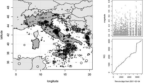The threshold magnitude of the catalog is $m_0=3$ resulting in 4100 earthquakes in the catalog. Figure 1 plots the earthquakes with the area of the circle indicating the relative size of the magnitude. The right plots contain the magnitude against occurrence time and cumulative count of earthquakes over the period.

Fig. 1 Left plot: Location of earthquakes in and around Italy from February 04, 2001 to March 28, 2020 with the area of the circle representing the relative size of the magnitude. Right plot: Cumulative number of earthquakes and dot-plot of magnitude against time.

Our proposed EM algorithm is used to estimate the RETAS model parameters for the Italian earthquake catalog. We fit RETAS models with Poisson, gamma renewal and Weibull renewal main-shock arrival processes where the gamma hazard rate function is given in (22), and the Weibull hazard rate function is given by (24) $$\mu (t)=\kappa \frac{t^{\kappa -1}}{{\beta }^{\kappa }},\hspace{1em}t\ge 0.$$(24)

We use a power-law temporal response function $g(t)=\frac{p-1}{c}{(1+\frac{t}{c})}^{-p}$ and exponential boost function $k(m)=A{e}^{\alpha (m-m_0)}$. With a Poisson arrival process, the model reduces to the classical ETAS model. We use the Akaike Information Criterion (AIC) to compare the three models. To fit the models, we sequentially apply the accelerated EM1 algorithm with progressively smaller tolerance parameters ϵ and δ which are set equal and take values $1\times {10}^{-2},1\times {10}^{-3},1\times {10}^{-4}$. In each iteration, the converged parameter value from the previous iteration is used as the starting value for the current iteration. In the final iteration, the exact EM1 algorithm is used to obtain the final estimate of the RETAS model parameters. The parameter estimates, their standard errors, and the AIC value are presented in Table 4. The standard errors were obtained by inverting the Hessian matrix computed at the EM estimate using the exact observed data log-likelihood in an additional step once the final estimate was obtained.

Table 4 Whole data EM algorithm estimation results for the Italian earthquake catalog with Poisson, gamma renewal, and Weibull renewal main-shock arrival processes.

	κ	β	p	c	A	α	AIC
Poisson	1.00	20.31	1.152	0.0189	0.625	1.143	267.01
	–	(4.133)	(0.0151)	(0.00266)	(0.0409)	(0.0507)
Gamma	0.498	20.58	1.181	0.0214	0.486	1.276	178.71
	(0.0345)	(2.823)	(0.0159)	(0.00306)	(0.0329)	(0.0551)
Weibull	0.646	3.96	1.229	0.0233	0.351	1.424	37.54
	(0.0180)	(0.330)	(0.0189)	(0.00330)	(0.0270)	(0.0600)

The parameter pairs $\left\{\kappa ,\beta \right\},\left\{p,c\right\}$, and $\left\{A,\alpha \right\}$ each describe a different feature of the earthquake sequence. The parameters κ and β describe the waiting time distribution between main-shocks. Since the gamma renewal and Weibull renewal processes are Poisson processes when their respective shape parameter κ is set equal to one it suggests that the RETAS models show a significant departure from the Poisson assumption of the ETAS model with an approximate 95% confidence interval for κ given by $(0.430,0.565)$ and $(0.611,0.681)$ for the gamma and Weibull models, respectively. The mean waiting time between main-shocks for the three models are 20.31, 10.24, and 5.45 for the Poisson, gamma, and Weibull models, respectively. 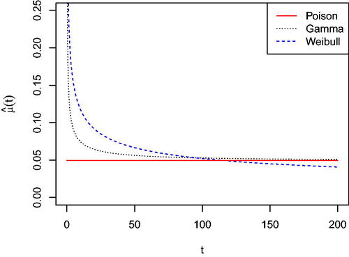Figure 2 plots the estimated hazard rate function $\widehat{\mu }(t)$ for the three models. The Poisson and the gamma hazard functions only differ in their short-term behavior with the longer-term hazard rate approaching similar levels. However, the estimated Weibull hazard function continues to decrease over the longer term and there is a noticeable difference in hazard rate for shorter waiting times. Both the gamma and Weibull hazard functions are monotonically decreasing from infinity with the Weibull hazard decreasing at a slower rate for smaller values of t.

Fig. 2 Estimated hazard function $\widehat{\mu }(t)$ for the RETAS models with Poisson, gamma renewal, and Weibull renewal main-shock processes for the Italian earthquake catalog.

The parameters p and c of the temporal response function g describe the temporal distribution of aftershocks relative to their triggering earthquake. The estimated parameters $\widehat{p}$ and $\widehat{c}$ for the three models are similar, although the Weibull model has aftershock effects that occur more rapidly after the triggering earthquake since it has the largest estimated $\widehat{p}$. The estimate of the magnitude density parameter is $\widehat{\gamma }=2.85$ and hence the productivity measure $\widehat{A}\widehat{\gamma }/(\widehat{\gamma }-\widehat{\alpha })$ is 1.043, 0.880, and 0.701 for the Poisson, gamma renewal and Weibull renewal models, respectively. This is consistent with the mean waiting time between main-shocks for the three models since for example the Weibull model has the smallest waiting time between main-shocks and hence has the smallest level of self-excitation effects.

The RETAS model with a Weibull renewal main-shock process is the preferred choice with a markedly smaller AIC value compared to the other two models. Indeed the Poisson main-shock process is not even a stationary model with a productivity that exceeds one. Hence, we conclude that the RETAS model outperforms the classical ETAS model and the whole data EM estimation method is able to avoid some of the convergence issues associated with direct maximization of the log-likelihood.

Supplementary Materials

The supplementary materials contain the code and data used in our real data analysis and we refer the reader to the readme file therein for details.

Acknowledgments

This research includes computations using the Linux computational cluster Katana supported by the Faculty of Science, UNSW Sydney, and the National Computational Infrastructure (NCI) supported by the Australian Government.

Disclosure Statement

No potential conflict of interest was reported by the author(s).

Additional information

Funding

Chen was partly supported by a UNSW SFRGP grant.

Appendix A.

Most Recent Immigrant Probabilities Conditional on the Whole Observed Data

Let $Y_{1:i-1}=\left\{{\tau }_{1:i-1},m_{1:i-1}\right\}$ be a subset of the observed data $Y=\left\{{\tau }_{1:n},m_{1:n},{\tau }_{n+1}>T\right\}$ and define ${\tau }_{i:n+1}$ to be $\left\{{\tau }_i,\dots ,{\tau }_n,{\tau }_{n+1}>T\right\}$. To calculate q_ij, we smooth the probabilities p_ij that facilitated likelihood evaluation in (4), by applying a suitable backward recursion. By applying Bayes’ theorem (A1) $$\begin{array}{c}{q}_{ij}=\frac{p({\tau }_{i:n+1}|Y_{1:i-1},I({\tau }_i)=j)}{p({\tau }_{i:n+1}|Y_{1:i-1})}·\mathbb{P}(I({\tau }_i)=j|Y_{1:i-1})\\ =\frac{p({\tau }_{i:n+1}|Y_{1:i-1},I({\tau }_i)=j)}{\sum _{k=1}^{i-1}p({\tau }_{i:n+1}|Y_{1:i-1},I({\tau }_i)=k)·p_{ik}}·p_{ij}.\end{array}$$(A1)

Define f_ij to be the joint density of ${\tau }_{i:n+1}$ conditional on $Y_{1:i-1}$ and $I({\tau }_i)=j$. Then it holds that (A2) $$\begin{array}{c}{f}_{ij}=p({\tau }_{i:n+1}|Y_{1:i-1},I({\tau }_i)=j)\\ =p({\tau }_i|Y_{1:i-1},I({\tau }_i)=j)·p({\tau }_{i+1:n+1}|Y_{1:i},I({\tau }_i)=j).\end{array}$$(A2)

The conditional density of the event time τ_i conditional on the previous times, marks and index of the most recent immigrant $I({\tau }_i)=j$ is given by (A3) $$\begin{array}{c}p({\tau }_i|Y_{1:i-1},I({\tau }_i)=j)\\ \hspace{1em}=(\mu ({\tau }_i-{\tau }_j)+\varphi ({\tau }_i))e^{-\{U({\tau }_i-{\tau }_j)-U({\tau }_{i-1}-{\tau }_j)\}-\{\Phi ({\tau }_i)-\Phi ({\tau }_{i-1})\}}.\end{array}$$(A3)

To calculate $p({\tau }_{i+1:n+1}|Y_{1:i},I({\tau }_i)=j)$ in (A2) we condition on the most recent immigrant at time ${\tau }_{i+1}$ denoted by $I({\tau }_{i+1})=k$ to obtain the following (A4) $$\begin{array}{c}\sum _{k=1}^{i}p({\tau }_{i+1:n+1}|Y_{1:i},I({\tau }_i)=j,I({\tau }_{i+1})=k)\\ \hspace{1em}·\mathbb{P}\left(I({\tau }_{i+1})=k|Y_{1:i},I({\tau }_i)=j\right).\end{array}$$(A4)

Since the conditioning information set contains both $I({\tau }_i)=j$ and $I({\tau }_{i+1})=k$, it implies that the only indexes contributing to the summation in (A4) are when k = j or k = i. Also, since we condition on the most recent immigrant at time ${\tau }_{i+1}$ we can remove $I({\tau }_i)=j$ from the conditioning information set since only the most recent renewal time provides information about the future evolution of the process given the history. Hence by the definition of f_ij, the summation in (A4) reduces to (A5) $$\sum _{k\in \left\{j,i\right\}}{f}_{i+1,k}·\mathbb{P}(I({\tau }_{i+1})=k|Y_{1:i},I({\tau }_i)=j).$$(A5)

The most recent immigrant index indicator function at time ${\tau }_{i+1}$, that is $I({\tau }_{i+1})$, is equal to $I({\tau }_i)$ if $B_i\ne 0$ or i if B_i = 0. Therefore, (A6) $$\begin{array}{c}\sum _{k\in \left\{j,i\right\}}{f}_{i+1,k}·\mathbb{P}(I({\tau }_{i+1})=k|Y_{1:i},I({\tau }_i)=j)\\ =[f_{i+1,j}·\mathbb{P}(I({\tau }_{i+1})=j|Y_{1:i},I({\tau }_i)=j)\\ +f_{i+1,i}·\mathbb{P}(I({\tau }_{i+1})=i|Y_{1:i},I({\tau }_i)=j)]\\ =[f_{i+1,j}·\mathbb{P}(B_i\ne 0|Y_{1:i},I({\tau }_i)=j)\\ +f_{i+1,i}·\mathbb{P}(B_i=0|Y_{1:i},I({\tau }_i)=j)]\\ =\left[f_{i+1,j}·\frac{\varphi ({\tau }_i)}{\mu ({\tau }_i-{\tau }_j)+\varphi ({\tau }_i)}+f_{i+1,i}·\frac{\mu ({\tau }_i-{\tau }_j)}{\mu ({\tau }_i-{\tau }_j)+\varphi ({\tau }_i)}\right]\end{array}$$(A6)

Hence, by substituting (A3) and (A6) into (A2) we obtain the following backward recursion to calculate f_ij (A7) $$f_{ij}=S_{ij}{e}^{-\{\Phi ({\tau }_i)-\Phi ({\tau }_{i-1})\}}\left[f_{i+1,j}·\varphi ({\tau }_i)+f_{i+1,i}·\mu ({\tau }_i-{\tau }_j)\right],$$(A7) with initial conditions $$\begin{array}{c}{f}_{n+1,j}=P({\tau }_{n+1}>T|{\tau }_{1:n},m_{1:n},I({\tau }_{n+1})=j)\\ =e^{-\{U(T-{\tau }_j)-U({\tau }_n-{\tau }_j)\}-\{\Phi (T)-\Phi ({\tau }_n)\}},\end{array}$$

for $j=1,\dots ,n.$

Appendix B.

Branching Structure Probabilities Conditioned on the Whole Observed Data

The recursive procedure to compute the most recent immigrant probabilities q_ij in Appendix A facilitates the calculation of the branching structure probabilities needed in the E-step. For the probabilities ω_ij we have (B1) $$\begin{array}{c}{\omega }_{ij}:=\mathbb{P}(B_i=0,I({\tau }_i)=j|Y)\\ =\mathbb{P}(B_i=0|Y,I({\tau }_i)=j)·\mathbb{P}(I({\tau }_i)=j|Y)\\ =\frac{\begin{array}{c}p({\tau }_{i+1:n+1},{\tau }_{n+1}>T|Y_{1:i},B_i=0,I({\tau }_i)=j)\hfill \\ ·\mathbb{P}(B_i=0|Y_{1:i},I({\tau }_i)=j)\hfill \end{array}}{p({\tau }_{i+1:n+1}|Y_{1:i},I({\tau }_i)=j)}·q_{ij}\\ =\frac{p({\tau }_{i+1:n+1}|Y_{1:i},I({\tau }_{i+1})=i)·\mathbb{P}(B_i=0|Y_{1:i},I({\tau }_i)=j)}{p({\tau }_{i+1:n+1}|Y_{1:i},I({\tau }_i)=j)}·q_{ij}.\end{array}$$(B1)

Hence, by the definition of $f_{i+1,j}$ and the expression provided in Appendix A, to compute the denominator in (A6), we obtain the following expression (B2) $${\omega }_{ij}=\frac{f_{i+1,i}·\mu ({\tau }_i-{\tau }_j)}{f_{i+1,j}·\varphi ({\tau }_i)+f_{i+1,i}·\mu ({\tau }_i-{\tau }_j)}·q_{ij}.$$(B2)

The parent probabilities conditional on the whole data Y required in the E-step can be calculated as follows $$\begin{array}{c}{\pi }_{ij}=\mathbb{P}\left(B_i=j|Y\right)\\ =\sum _{k=1}^{i-1}\mathbb{P}(B_i=j|Y,I({\tau }_i)=k)·q_{ik}\\ =\sum _{k=1}^{i-1}\frac{\begin{array}{c}p({\tau }_{i+1:n+1}|Y_{1:i},I({\tau }_i)=k,B_i=j)\hfill \\ ·\mathbb{P}(B_i=j|Y_{1:i},I({\tau }_i)=k)\hfill \end{array}}{p({\tau }_{i+1:n+1}|Y_{1:i},I({\tau }_i)=k)}·q_{ik}.\end{array}$$

Again, the denominator was computed in (A6), and using the definition of f_ij we obtain the following (B3) $${\pi }_{ij}=\sum _{k=1}^{i-1}\frac{f_{i+1,k}·\psi ({\tau }_i-{\tau }_j,m_j)}{f_{i+1,k}·\varphi ({\tau }_i)+f_{i+1,i}·\mu ({\tau }_i-{\tau }_k)}·q_{ik}.$$(B3)

References

- Chen, F., and Stindl, T. (2018), “Direct Likelihood Evaluation for the Renewal Hawkes Process,” Journal of Computational and Graphical Statistics, 27, 119–131. DOI: 10.1080/10618600.2017.1341324.
- Daley, D. J., and Vere-Jones, D. (2003), An Introduction to the Theory of Point Processes. Springer Series in Statistics. New York: Springer.
- Dempster, A. P., Laird, N. M., and Rubin, D. B. (1977), “Maximum Likelihood from Incomplete Data via the EM Algorithm,” Journal of the Royal Statistical Society, Series B, 39, 1–38. DOI: 10.1111/j.2517-6161.1977.tb01600.x.
- Guo, Y., Zhuang, J., and Zhou, S. (2015), “An Improved Space-Time ETAS Model for Inverting the Rupture Geometry from Seismicity Triggering,” Journal of Geophysical Research (Solid Earth), 120, 3309–3323. DOI: 10.1002/2015JB011979.
- Gutenberg, B., and Richter, C. F. (1944), “Frequency of Earthquakes in California,” Bulletin of the Seismological Society of America, 34, 185–188. DOI: 10.1785/BSSA0340040185.
- Halpin, P. F. (2013), “A Scalable EM Algorithm for Hawkes Processes,” in New Developments in Quantitative Psychology: Presentations from the 77th Annual Psychometric Society Meeting, eds. R. E. Millsap, L. A. van der Ark, D. M. Bolt, and C. M. Woods, pp. 403–414, New York: Springer.
- Hawkes, A. G. (1971), “Spectra of Some Self-Exciting and Mutually Exciting Point Processes,” Biometrika, 58, 83–90. DOI: 10.1093/biomet/58.1.83.
- Hawkes, A. G., and Oakes, D. (1974), “A Cluster Process Representation of a Self-Exciting Process,” Journal of Applied Probability, 11, 493–503. DOI: 10.2307/3212693.
- Jamshidian, M., and Jennrich, R. I. (1997), “Acceleration of the EM Algorithm by Using Quasi-Newton Methods,” Journal of the Royal Statistical Society, Series B, 59, 569–587. DOI: 10.1111/1467-9868.00083.
- Jamshidian, M., and Jennrich, R. I. (2000), “Standard Errors for EM Estimation,” Journal of the Royal Statistical Society, Series B, 62, 257–270. DOI: 10.1111/1467-9868.00230.
- Lewis, E., and Mohler, G. (2011), “A Nonparametric EM Algorithm for Multiscale Hawkes Processes,” Journal of Nonparametric Statistics, 1(1):1–20.
- Lin, F., and Fine, J. P. (2009), “Pseudomartingale Estimating Equations for Modulated Renewal Process Models,” Journal of the Royal Statistical Society, Series B, 71, 3–23. DOI: 10.1111/j.1467-9868.2008.00680.x.
- Marsan, D., and Lengliné, O. (2008), “Extending Earthquakes’ Reach through Cascading,” Science, 319, 1076–1079. DOI: 10.1126/science.1148783.
- Meyer, S., Elias, J., and Höhle, M. (2012), “A Space–Time Conditional Intensity Model for Invasive Meningococcal Disease Occurrence,” Biometrics, 68, 607–616. DOI: 10.1111/j.1541-0420.2011.01684.x.
- Mohler, G. O., Short, M. B., Brantingham, P. J., Schoenberg, F. P., and Tita, G. E. (2011), “Self-Exciting Point Process Modeling of Crime,” Journal of the American Statistical Association, 106, 100–108. DOI: 10.1198/jasa.2011.ap09546.
- Molkenthin, C., Donner, C., Reich, S., Zöller, G., Hainzl, S., Holschneider, M., and Opper, M. (2022), “GP-ETAS: Semiparametric Bayesian Inference for the Spatio-Temporal Epidemic Type Aftershock Sequence Model,” Statistics and Computing, 32, 29. DOI: 10.1007/s11222-022-10085-3.
- Nelder, J. A., and Mead, R. (1965), “A Simplex Method for Function Minimization,” The Computer Journal, 7, 308–313. DOI: 10.1093/comjnl/7.4.308.
- Ogata, Y. (1988), “Statistical Models for Earthquake Occurrences and Residual Analysis for Point Processes,” Journal of the American Statistical Association, 83, 9–27. DOI: 10.1080/01621459.1988.10478560.
- ———(1998), “Space-Time Point-Process Models for Earthquake Occurrences,” Annals of the Institute of Statistical Mathematics, 50, 379–402.
- Ogata, Y., and Zhuang, J. (2006), “Space–Time ETAS Models and an Improved Extension,” Tectonophysics, 413, 13–23. Critical Point Theory and Space-Time Pattern Formation in Precursory Seismicity. DOI: 10.1016/j.tecto.2005.10.016.
- Omori, F. (1894), “On the Aftershocks of Earthquakes,” Jounal of the College of Science, Imperial University of Tokyo, 7, 111–120.
- Stindl, T., and Chen, F. (2019), “Modeling Extreme Negative Returns Using Marked Renewal Hawkes Processes,” Extremes, 22, 705–728. DOI: 10.1007/s10687-019-00352-4.
- ———(2021), “Accelerating the Estimation of Renewal Hawkes Self-Exciting Point Processes,” Statistics and Computing, 31, 26.
- ———(2022), “Spatiotemporal ETAS Model with a Renewal Main-Shock Arrival Process,” Journal of the Royal Statistical Society, Series C, 71, 1356–1380.
- ———(2023), “Stochastic Declustering of Earthquakes with the Spatiotemporal RETAS Model,” Annals of Applied Statistics. Forthcoming.
- Utsu, T. (1961), “A Statistical Study of the Occurrence of Aftershocks,” Geophysical Magazine, 30, 521–605.
- Veen, A., and Schoenberg, F. P. (2008), “Estimation of Space–Time Branching Process Models in Seismology Using an EM–Type Algorithm,” Journal of the American Statistical Association, 103, 614–624. DOI: 10.1198/016214508000000148.
- Wheatley, S., Filimonov, V., and Sornette, D. (2016), “The Hawkes Process with Renewal Immigration & its Estimation with an EM Algorithm,” Computational Statistics & Data Analysis, 94, 120–135. DOI: 10.1016/j.csda.2015.08.007.
- Zhuang, J., and Mateu, J. (2019), “A Semiparametric Spatiotemporal Hawkes-Type Point Process Model with Periodic Background for Crime Data,” Journal of the Royal Statistical Society, Series A, 182, 919–942. DOI: 10.1111/rssa.12429.