Convolutional Neural Networks for Valid and Efficient Causal Inference

Abstract

Convolutional neural networks (CNN) have been successful in machine learning applications. Their success relies on their ability to consider space invariant local features. We consider the use of CNN to fit nuisance models in semiparametric estimation of the average causal effect of a treatment. In this setting, nuisance models are functions of pretreatment covariates that need to be controlled for. In an application where we want to estimate the effect of early retirement on a health outcome, we propose to use CNN to control for time-structured covariates. Thus, CNN is used when fitting nuisance models explaining the treatment and the outcome. These fits are then combined into an augmented inverse probability weighting estimator yielding efficient and uniformly valid inference. Theoretically, we contribute by providing rates of convergence for CNN equipped with the rectified linear unit activation function and compare it to an existing result for feedforward neural networks. We also show when those rates guarantee uniformly valid inference. A Monte Carlo study is provided where the performance of the proposed estimator is evaluated and compared with other strategies. Finally, we give results on a study of the effect of early retirement on hospitalization using data covering the whole Swedish population. Supplementary materials are available online at https://github.com/stat4reg/Causal/_CNN.

KEYWORDS:

• Augmented inverse probability weighting
• Average causal effect
• Early retirement
• Post-machine learning inference

1 Introduction

Convolutional Neural Networks (CNN) have been found successful in discovering location-invariant patterns in speech, images, and time series data (LeCun and Bengio 1995). In particular, they have been shown to have a universal approximation property and be more efficient in terms of number of hidden layers than fully connected multi-layer networks in high-dimensional situations (Zhou 2020). In this article we show how CNN can be useful in controlling confounding information, including location-invariant patterns in time series, in order to perform semiparametric inference on a low dimensional causal parameter: we focus on average causal effects of a binary treatment on an outcome of interest, although our results are relevant for the semiparametric estimation of other low dimensional parameters of interest (see e.g., Chernozhukov et al. 2018).

Augmented Inverse Probability Weighting (AIPW) estimators (also called Double Robust (DR) estimators, Robins, Rotnitzky, and Zhao 1994) attain the semiparametric efficiency bound and yield uniformly valid inference as long as the nuisance functions of the confounding covariates are fitted consistenlty with fast enough convergence rates; for example, all nuisance functions are estimated with order $n^{-1/4}$ (Belloni, Chernozhukov, and Hansen 2014; Farrell 2015; Kennedy 2016; Moosavi, Häggström, and de Luna 2021). In this article, we contribute to this theory by showing that CNN fits of nuisance functions achieve the $n^{-1/4}$ convergence rate required to obtain uniformly valid inference on causal parameters. To show this we use a result obtained by Farrell, Liang, and Misra (2021) for Rectified Linear Unit (ReLU)-based Feed-forward Neural Networks (FNN). They show that, for large samples, the estimation error rate of FNN are bounded by the following term, with a probability at least $1-e^{-\gamma }$: (1) $$\begin{array}{c}\sqrt{\hspace{0.17em}\log \hspace{0.17em}n/n}\times \text{Model complexity}+\sqrt{(\hspace{0.17em}\log \hspace{0.17em}\hspace{0.17em}\log \hspace{0.17em}n+\gamma )/n}\\ \mathrm{\hspace{1em}}\mathrm{\hspace{1em}}+\text{approximation rate}.\end{array}$$(1)

We deduce the above approximation rate for CNN architectures inspired by earlier work by Zhou (2020). However, in contrast to the latter paper, we consider a larger number of free parameters by considering multi-channel convolutional neural network, so as to achieve a tradeoff between complexity penalty of the function class and approximation rate in (1), and thereby obtain the convergence rate $n^{-1/4}$ for the CNN fit of the nuisance functions.

In the next section we formally define the causal parameters of interest using the potential outcome framework (Rubin 1974), and introduce the assumptions yielding identification, and locally efficient and uniformly valid inference when using AIPW estimators. We also introduce the convolutional network architectures with which we propose to fit the nuisance functions used by AIPW, followed by our main theoretical results, including conditions to obtain uniformly valid inference when using CNN based AIPW estimation. Section 3 presents numerical experiments illustrating the finite sample behavior of this estimation strategy under different data generating mechanisms. The proposed estimator is compared to AIPW, Targeted Maximum Likelihood Estimation (TMLE) (van der Laan and Rose 2011) and Outcome Regression (OR) estimation (Tan 2007; Moosavi, Häggström, and de Luna 2021) using fully-connected feed-forward ReLU based neural networks (Multilayer Perceptron (MLP) in Farrell, Liang, and Misra, 2021) and Lasso to fit the nuisance functions. In Section 4, we study the effect of early retirement (at 62 years old), compared to retiring later in life, on morbidity and mortality outcomes (Barban et al. 2020). We use population wide Swedish register data and follow cohorts born in 1946 and 1947 for which we have a rich reservoir of potential pretreatment confounders, including hospitalization and income histories. CNN allows us to consider that such life histories may contain location-invariant patterns that confound the causal effects of the treatment (decision to retire early).

2 Theory and Method

2.1 Causal Parameters and Uniformly Valid Inference

The Average Causal Effect (ACE) and Average Causal Effect among the Treated (ACET) of a binary treatment (T) are parameters defined using potential outcomes ((Rubin 1974)), respectively: $$\begin{array}{c}\tau =\mathbb{E}(Y(1))-\mathbb{E}(Y(0)),\\ {\tau }_t=\mathbb{E}(Y(1)-Y(0)|T=1),\end{array}$$where Y(1) and Y(0) are the outcomes that would be observed if T = 1 and T = 0, respectively. For a given individual only one of these potential outcomes can be observed. This intrinsic missing data problem implies that assumptions need to be made to identify τ and τ_t. For this purpose, and given a vector of observed pretreatment covariates X, we assume:

Assumption 1.

1. No unmeasured confounders:

   1. $Y(0)\perp \mathrm{}\mathrm{}\perp T|X$.

   2. $Y(1)\perp \mathrm{}\mathrm{}\perp T|X$.

2. Overlap:

   1. $\mathbb{P}(T=0|X)>0$.

   2. $\mathbb{P}(T=1|X)>0$.

3. Consistency: The observed outcome is $Y=Y(1)T+Y(0)(1-T).$

Note that ACET is identified if only 1a(i), 1b(i), and 1c hold. Assumption 1a requires that the observed vector X includes all confounders. Assumption 1b requires that for any value X both treatment levels have nonzero probability to occur, and by Assumption 1c one of the potential outcomes is observed for each individual, and its value is not affected by the treatment received by other individuals in the sample.

We aim at uniformly (over the class of Data Generating Processs (DGP)s, for which Assumption 2 hold) valid inference while using semiparametric estimation (Moosavi, Häggström, and de Luna 2021). Therefore, the following AIPW estimators of ACE are considered (Robins, Rotnitzky, and Zhao 1994; Scharfstein, Rotnitzky, and Robins 1999): $$\widehat{\tau }={\mathbb{E}}_n[{\widehat{\psi }}_1(z_i)-{\widehat{\psi }}_0(z_i)]$$where ${\mathbb{E}}_n[·]$ is the empirical mean operator, $${\widehat{\psi }}_t(z_i)=\frac{\mathbb{1}\{t_i=t\}(y_i-{\widehat{\mu }}_t(x_i))}{\widehat{\mathbb{P}}[T=t|X=x_i]}+{\widehat{\mu }}_t(x_i),$$ and ${\widehat{\mu }}_t(x)$ is an estimator of ${\mu }_t(x)=\mathbb{E}(Y(t)|X=x)$.

For ACET, we use the estimator ${\widehat{\tau }}_t={\mathbb{E}}_n[{\widehat{\psi }}_{1,1}(z_i)-{\widehat{\psi }}_{0,1}(z_i)],$ where $$\begin{array}{c}{\widehat{\psi }}_{t,t\prime }(z_i)=\frac{\widehat{\mathbb{P}}[T=t\prime |X=x_i]}{\widehat{\mathbb{P}}[T=t\prime ]}\frac{\mathbb{1}\{t_i=t\}(y_i-{\widehat{\mu }}_t(x_i))}{\widehat{\mathbb{P}}[T=t|X=x_i]}\\ +\frac{\mathbb{1}\{t_i=t\prime \}{\widehat{\mu }}_t(x_i)}{\widehat{\mathbb{P}}[T=t\prime ]}.\end{array}$$

We use the following assumptions for the DGP’.

Assumption 2.

We have

1. Let $\{(y_i,t_i,x_i),i=1,\dots ,n\}$ be an iid sample from (Y, T, X).

2. Let $U=Y(t)-{\mu }_t(X)$. There is some r > 0 for which $\mathbb{E}({\left|{\mu }_t(x_i){\mu }_{t^{\prime }}(x_i)\right|}^{1+r})$ and $\mathbb{E}({\left|u_i\right|}^{4+r})$ are bounded, for given values of t and $t\prime$.

The estimators of the nuisance functions have yet to be introduced for these AIPW estimation strategies. In order to get the desired results, the proposed estimators should be well behaved. More precisely, the following consistency and rate conditions are considered for the nuisance function estimators.

Assumption 3.

Let $\widehat{p}(x)$ be an estimator of $\mathbb{P}[T=1|X=x_i]$ which only depends on ${\{x_i,t_i\}}_{i=1}^n$ (assumption of “no additional randomness,” Farrell 2015). Moreover, for a given t we have

1. ${\mathbb{E}}_n[{(\widehat{p}(x_i)-p(x_i))}^2]=o_P(1)$ and ${\mathbb{E}}_n[{({\widehat{\mu }}_t(x_i)-{\mu }_t(x_i))}^2]=o_P(1),$

2. ${\mathbb{E}}_n{[{({\widehat{\mu }}_t(x_i)-{\mu }_t(x_i))}^2]}^{1/2}{\mathbb{E}}_n{[{(\widehat{p}(x_i)-p(x_i))}^2]}^{1/2}=o_P(n^{-1/2}),$

3. ${\mathbb{E}}_n[({\widehat{\mu }}_t(x_i)-{\mu }_t(x_i))(1-\mathbb{1}\{t_i=t\}/\mathbb{P}[T=t|X=x_i])]=o_P(n^{-1/2})$.

The following proposition describes uniform validity results obtained by Farrell (2018, Corollaries 2 and 3) under the above regularity conditions.

Proposition 1.

For each n, let ${\mathcal{P}}_n$ be the set of distributions obeying Assumptions 1a(i), 1b(i), 1c, and 2a. Further, assume Assumption 2b holds for $t=t\prime =0$, and let $\widehat{p}(x)$ and ${\widehat{\mu }}_0(x)$ fulfill Assumption 3. Then, we have: $$\begin{array}{c}\underset{P\in {\mathcal{P}}_n}{\sup }\left|{\mathbb{P}}_P\left({\tau }_t\in \left\{{\widehat{\tau }}_t\pm c_{\alpha }\sqrt{{\widehat{V}}_t/n}\right\}\right)-\left(1-\alpha \right)\right|\to 0,\hfill \end{array}$$where $$\begin{array}{c}{\widehat{V}}_t=\frac{n^2}{n_t^2}{\mathbb{E}}_n\left[\mathbb{1}(t_i=1){\left(y_i-{\widehat{\mu }}_0\left(x_i\right)-{\widehat{\tau }}_t\right)}^2\right]\\ \mathrm{\hspace{1em}}\mathrm{\hspace{1em}}+\frac{n^2}{n_t^2}{\mathbb{E}}_n\left[\frac{\widehat{p}{\left(x_i\right)}^2}{{\left(1-\widehat{p}\left(x_i\right)\right)}^2}\mathbb{1}(t_i=0){\left(y_i-{\widehat{\mu }}_0\left(x_i\right)\right)}^2\right],\end{array}$$

$n_t={\Sigma }_{i=1}^n\mathbb{1}(T=t)$ and $c_{\alpha }={\Phi }^{-1}(1-\alpha /2)$.

Let also Assumptions 1a(ii), 1b(ii) be fulfilled and Assumption 2b hold for $t,t\prime \in \{0,1\}$. Additionally, assume ${\widehat{\mu }}_1(x)$ fulfills Assumption 3. Then, we have: $$\begin{array}{c}\underset{P\in {\mathcal{P}}_n}{\sup }\left|{\mathbb{P}}_P\left(\tau \in \left\{\widehat{\tau }\pm c_{\alpha }\sqrt{\widehat{V}/n}\right\}\right)-\left(1-\alpha \right)\right|\to 0,\hfill \end{array}$$where $$\begin{array}{cc}\widehat{V}\hfill & ={\mathbb{E}}_n\left[\frac{\mathbb{1}(t_i=1){\left(y_i-{\widehat{\mu }}_1\left(x_i\right)\right)}^2}{\widehat{p}{\left(x_i\right)}^2}\right]\hfill \\ \hfill & \mathrm{\hspace{1em}}\mathrm{\hspace{1em}}+{\mathbb{E}}_n\left[{\left({\widehat{\mu }}_1\left(x_i\right)-{\mathbb{E}}_n[{\widehat{\psi }}_1(z_i)]\right)}^2\right]\hfill \\ \hfill & +{\mathbb{E}}_n\left[\frac{\mathbb{1}(t_i=0){\left(y_i-{\widehat{\mu }}_0\left(x_i\right)\right)}^2}{{\left(1-\widehat{p}\left(x_i\right)\right)}^2}\right]\hfill \\ \hfill & \mathrm{\hspace{1em}}\mathrm{\hspace{1em}}+{\mathbb{E}}_n\left[{\left({\widehat{\mu }}_0\left(x_i\right)-{\mathbb{E}}_n[{\widehat{\psi }}_0(z_i)]\right)}^2\right].\hfill \end{array}$$

Remark 1.

A multiplicative rate condition as Assumption 3(b) is weaker than separate conditions on the two nuisance model estimators. It only requires that one of the nuisance functions is estimated at faster rate if the other one is estimated at slower rate. However, in Section 2.3 the rate $o_P(n^{-1/4})$ is obtained for each of the nuisance function estimators separately. This is to make sure Assumption 3(c) for $\widehat{\mu }$ is also fulfilled. This latter assumption can be, however, dropped by considering sample splitting (Chernozhukov et al. 2018).

Assumption 3, or similar condition, has been used in the literature to obtain uniform valid inference of average causal effect estimators; see Belloni, Chernozhukov, and Hansen (2014), Farrell (2015), Farrell, Liang, and Misra (2021), Chernozhukov et al. (2018), and van der Laan and Rose (2011). Machine learning algorithms estimating regression functions with rate $o_P(n^{-1/4})$ include regression trees, lasso regressions, and neural networks (see (Kennedy 2016; Chernozhukov et al. 2018) for an overview). Concerning the neural networks, $o(n^{-1/4})$ rate of convergence was shown for shallow and deep feed-forward neural networks in Chen and White (1999) and Farrell, Liang, and Misra (2021), respectively. Note, finally, that because the AIPW estimators is based on the efficient influence function, its asymptotic variance is equal to the semiparametric efficiency bound (Tsiatis 2006).

2.2 Convolutional Neural Networks

We consider a specific CNN architecture with parallel hidden layers structured as follows. Let the input column vector be denoted by $h^0:=(x_1,\dots ,x_d)\prime \in \Omega$, where $\Omega \subseteq {\mathbb{R}}^d$. We consider L to be the number of hidden layers in which we have E number of parallel vectors. Let σ be the ReLU function defined on the space of real numbers as $\sigma (z)=\max (0,z)$ for $z\in \mathbb{R}$. The vectors in each hidden layer $l\in \{1,\dots ,Ł\}$ have size d_l and are defined by $h_e^l=\sigma (W_e^l{h}_e^{l-1}-b_l^e)$, where $e\in \{1,\dots ,E\},h_e^0=h^0,b_l^e$ is a vector called bias vector in the neural network literature, $W_e^l$ is a weight matrix defined as $$W_e^l=\left[\begin{array}{cccccc}{w}_{0,l}^e& 0& 0& 0& \cdots & 0\\ w_{1,l}^e& w_{0,l}^e& 0& 0& \cdots & 0\\ ⋮& \ddots & \ddots & \ddots & \cdots & ⋮\\ w_{s,l}^e& w_{s-1,l}^e& \cdots & w_{0,l}^e& 0\cdots & 0\\ 0& w_{s,l}^e& w_{s-1,l}^e& \cdots & w_{0,l}^e\cdots & 0\\ ⋮& \ddots & \ddots & \ddots & \cdots & ⋮\\ ⋮& \cdots & 0& w_{s,l}^e& \cdots & w_{0,l}^e\\ ⋮& \cdots & \cdots & 0& w_{s,l}^e\cdots & w_{1,l}^e\\ ⋮& \ddots & \ddots & \ddots & \ddots & ⋮\\ 0& \cdots & \cdots & \cdots & 0\hspace{1em}{w}_{s,l}^e& w_{s-1,l}^e\\ 0& \cdots & \cdots & \cdots & \cdots 0& w_{s,l}^e\end{array}\right],$$and the weight parameter $w_{i,l}^e$ is the ith element of the filter mask $(w_{0,l}^e,\dots ,w_{s,l}^e)$. s is considered fixed through all values of l and e. We have $d_l=d_0+sl$, where d_l is the size of vectors in the lth layer and $d_0=d$.

The structure of a CNN as defined above provides us with the following function space on Ω: $$\mathcal{C}=\left\{\sum _{e=1}^E{c}_e^{\prime }{h}_e^L:c_e\in {\mathbb{R}}^{d_L}\right\}.$$

Similar to Zhou (2020) (who, however, uses E = 1) we assume that for all values of e in $\{1,\dots E\}$ and l in $\{1,\dots ,L-1\}$ the vector $b_l^e$ has the form $(b_{l,1}^e,\dots ,b_{l,s}^e,b_{l,s+1}^e,\dots ,b_{l,s+1}^e,b_{l,d_l-s+1}^e,\dots ,b_{l,d_l}^e)\prime$ with the $d_l-2s$ repeated components in the middle. Therefore, the total number of parameters (duplicate/shared weights are counted more than once), Q for the neural network fulfills the following inequality: (2) $$Q=E(d(1+s)(L-1)+s(1+s)L(L-1)/2+(s+3)(d+sL))\asymp E{L}^2,$$(2) where the notation $x_n\asymp y_n$ for two sequences of random variables x_n and y_n means $x_n=O_P(y_n)$ and $y_n=O_P(x_n)$.

2.3 Main Results

In this section, we provide results that allow us to use the CNN architectures described above to fit the nuisance models needed for AIPW estimations of ACE and ACET, and obtain uniformly valid inference. In particular, we need to show that the rate conditions in Assumption 3 are fulfilled.

Assumption 4.

Assume that $z_i=(u_i^T,v_i),1\le i\le n$ are iid copies of $Z=(U,V)\in {[-1,1]}^d\times \mathcal{V}$, where U is continuously distributed. For an absolute constant M > 0 and a target $f^{*}$ (a nuisance function), assume $\mathcal{V}\in [-M,M]$ and ${\Vert f^{*}\Vert }_{\infty }\le M$.

Assumption 5.

Let $\mathcal{l}$ be a loss function that, for any arbitrary functions f and g and z a realization of Z, fulfills: $$\begin{array}{cc}\hfill & |\mathcal{l}(f,z)-\mathcal{l}(g,z)|\le C_{\mathcal{l}}|f(x)-g(x)|,\hfill \\ \hfill & c_1\mathbb{E}({(f-\tilde{f})}^2)\le \mathbb{E}(\mathcal{l}(f,Z))-\mathbb{E}(\mathcal{l}(\tilde{f},Z))\le c_2\mathbb{E}({(f-\tilde{f})}^2),\hfill \end{array}$$where $\tilde{f}=\text{arg} \min \mathbb{E}(\mathcal{l}(\mathrm{f},\mathrm{Z}))$.

Note that Assumption 5 holds for the usual mean squared error and log loss functions. Further, let $\mathcal{F}$ be an arbitrary set of functions. We define: (3) $${\widehat{f}}_{\mathcal{F}}:=\underset{\stackrel{f\in \mathcal{F}}{{\Vert f\Vert }_{\infty }\le M\prime }}{\text{arg} \min }\sum _{i=1}^n\mathcal{l}(f,z),$$(3) and (4) $${\epsilon }_{\mathcal{F},\mathcal{F}\prime }:=\underset{\stackrel{f\in \mathcal{F}}{}}{\sup }\underset{\stackrel{f\prime \in \mathcal{F}\prime }{{\Vert f\prime \Vert }_{\infty }\le M\prime }}{\inf }{\Vert f-f\prime \Vert }_{\infty },$$(4) where ${\Vert ·\Vert }_{\infty }$ is the supremum norm. The following result is a special case of Theorem 2(b) given in Farrell, Liang, and Misra (2021), and gives the rate of convergence for our estimate ${\widehat{f}}_{\mathcal{C}}$ of a target $f^{*}$ (a nuisance function). Prior to presenting the theorem, the target space in which we seek to find the nuisance functions need to be defined. We use the notation $W^{\beta ,\infty }(\Omega )$ for the Sobolev space with smoothness $\beta \in {\mathbb{N}}_{+}$. We consider $\mathcal{W}$ to be the unit ball in the Sobolev space defined on ${[-1,1]}^d$; $\mathcal{W}:=B_1(W^{\beta ,\infty }({[-1,1]}^d))$ such as $$\mathcal{W}:=\{f:\underset{{}_{\stackrel{\alpha ,\left|\alpha \right|\le \beta }{}}}{\max }{\Vert D^{\alpha }f(x)\Vert }_{L^{\infty }({[-1,1]}^d)}\le 1\},$$ where ${\Vert f\Vert }_{L^{\infty }(\Omega )}$ is the essential supremum norm of the absolute value of a function f defined on Ω, $\alpha =({\alpha }_1,\dots ,{\alpha }_d)\prime ,\left|\alpha \right|={\alpha }_1+\cdots +{\alpha }_d$, and $D^{\alpha }f$ is the weak derivative.

Theorem 1.

Let $f^{*}\in \mathcal{W}$, and assume that Assumptions 4-5 hold. For an absolute constant M > 0 and $M\prime =2M$, let the approximation error ${\epsilon }_{\mathcal{W},\mathcal{C}}$ be defined as in (4). With probability at least $1-e^{-\gamma }$, and for large enough n, (5) $$\begin{array}{c}{\mathbb{E}}_n\left[{({\widehat{f}}_{\mathcal{C}}-f^{*})}^2\right]\le C(\frac{QL\hspace{0.17em}\log \hspace{0.17em}Q}{n}\log \hspace{0.17em}n+\frac{\hspace{0.17em}\log \hspace{0.17em}\hspace{0.17em}\log \hspace{0.17em}n+\gamma }{n}+{\epsilon }_{\mathcal{W},\mathcal{C}}^2),\hfill \end{array}$$(5) where the constant C > 0 is independent of n, but may depend on d, M, and other fixed constants.

Our next step is to bound the term ${\epsilon }_{\mathcal{W},\mathcal{C}}^2$ in the above inequality on the estimation error. The following result is similar to Theorem 1 in Zhou (2020). However, we allow here the number of parallel layers to grow with n, which translates into faster growing function space for our specific CNN architectures, thereby a larger decay rate for the error.

Theorem 2.

Let $2\le s\le d$. If $L\ge 2d/(s-1)$ and $f\in \mathcal{W}$, ${\Vert f\Vert }_{\infty }\le M$ and an integer index $\beta >2+d/2$, then there exist w, b and $f_{L,E}^{w,b}\in \mathcal{C}$ such that $${\Vert f-f_{L,E}^{w,b}\Vert }_{C({[-1,1]}^d)}\le c{2}^{d/2}\sqrt{\hspace{0.17em}\log \hspace{0.17em}(LE)}{(LE)}^{-\frac{1}{2}-\frac{1}{d}},$$

where $C({[-1,1]}^d)$ is the space of continuous functions on the space ${[-1,1]}^d$ and c is an absolute constant and therefore $${\epsilon }_{\mathcal{W},\mathcal{C}}\le C\sqrt{\hspace{0.17em}\log \hspace{0.17em}(LE)}{(LE)}^{-\frac{1}{2}-\frac{1}{d}}.$$

Note that this theorem holds under more general Sobolev spaces for f. For simplicity, we use the condition $f\in \mathcal{W}$ because it is necessary in the other theorems in this section.

Finally, our main result gives conditions for the CNN nuisance function fit to fulfill Assumption 3, and therefore conditions for AIPW estimation based on CNN fit to yield uniformly valid inference for ACE and ACET (Proposition 1).

Theorem 3.

Let the conditions in Theorem 1 hold for u_i = x_i, v_i = y_i, and $f^{*}={\mu }_t\in \mathcal{W}$ with smoothness ${\beta }_{\mu }$. Let also the same conditions hold for u_i = x_i, v_i = t_i, and $f^{*}=p\in \mathcal{W}$ with smoothness β_p. Let also $E\asymp n^{\frac{d}{2d+4}},L\asymp n^{\frac{1}{4d+8}}{\hspace{0.17em}\log \hspace{0.17em}}^2(n),\beta ={\beta }_p\wedge {\beta }_{\mu }$, and s and d fulfill the assumptions of Theorem 2. Then, the rate conditions in Assumption 3 are fulfilled for nuisance functions estimators (3) with $\mathcal{F}=\mathcal{C}$ and any loss function $\mathcal{l}$ that fulfills Assumption 5.

Remark 2.

The rate result for CNN based estimators in Theorem 3 corresponds to similar results for MLP in Farrell, Liang, and Misra (2021, Theorem 3). However, the conditions on smoothness is less strict in our case. Moreover, the rate of growth for the number of parameters considered for MLP based estimators in Farrell, Liang, and Misra (2021, Theorem 1) is $n^{\frac{d}{\beta +d}}{\hspace{0.17em}\log \hspace{0.17em}}^{5}n$, while we have considered the growth rate $n^{\frac{d+1}{2d+4}}{\hspace{0.17em}\log \hspace{0.17em}}^4(n)$. These rates are similar up to a log factor if d is large and β is close to d. Notice, however, that these are not necessarily minimal rates required for valid inference on ACE(T).

Remark 3.

We have assumed that both width E and depth L are growing at given rates. One interesting question is what happens if we consider one of them constant and only grew the other? It is not difficult to check that assuming constant E, and $L=n^{\alpha }$, gives us the following result: $$\begin{array}{cc}\hfill & {\mathbb{E}}_n\left[{({\widehat{f}}_{\mathcal{C}}-f^{*})}^2\right]\hfill \\ \hfill & \le C(\frac{n^{3\alpha }\hspace{0.17em}\log \hspace{0.17em}{n}^{2\alpha }}{n}\log \hspace{0.17em}n+\frac{\hspace{0.17em}\log \hspace{0.17em}\hspace{0.17em}\log \hspace{0.17em}n+\gamma }{n}+\hspace{0.17em}\log \hspace{0.17em}(n^{\alpha })n^{-\alpha \frac{2+d}{d}}).\hfill \end{array}$$

Therefore, establishing a convergence rate of $o_p(n^{-1/4})$ for ${\mathbb{E}}_n[{({\widehat{f}}_{\mathcal{C}}-f^{*})}^2]$ requires each of these terms to have a growth rate smaller than $-\frac{1}{2}$. This implies for the first term: $3\alpha -1<-\frac{1}{2}\Rightarrow \alpha <\frac{1}{6}$, and for the third one: $-\alpha \frac{2+d}{d}<-\frac{1}{2}\Rightarrow \alpha >\frac{d}{2(2+d)}$. Thus, for a proper candidate for α we need: $\frac{d}{2(2+d)}<\frac{1}{6}\Rightarrow d<1$, which contradicts the assumption d > 2. Hence, E cannot be kept fixed here.

3 Simulation Study

We perform a simulation study to evaluate the use of the CNN together with AIPW estimation strategy of average causal effects proposed above. We focus here on τ_t (ACET) but similar results are obtained for τ. Comparisons are made with other algorithms to fit nuisance functions, including, MLP, (Farrell, Liang, and Misra 2021) and post-lasso estimators (Farrell 2015). Moreover, we also include alternative strategies to AIPW, including OR estimation (Tan 2007) and targeted learning (van der Laan and Rose 2011).

The simulation results are based on 1000 replications. The neural networks initial weights are different for each replication, which makes the results more robust. A sequence of 10 covariates are independently generated having normal distributions with increasing means and varying variances: $X_1\sim N(100,20),X_2\sim N(102,15),X_3\sim N(105,13),X_4\sim N(107,11),X_5\sim N(109,8),X_6\sim N(110,20),X_7\sim N(112,15),X_8\sim N(115,13),X_9\sim N(117,11)$, and $X_{10}\sim N(119,8)$. While these variables are independent, their ordering is going to be important in how the outcomes and treatment assignment are generated as described below in two different settings.

Setting 1 Potential outcomes and treatment assignment are generated as follows: $$\begin{array}{c}Y(0)=1+0.001({(X_2-X_1)}^2+{(X_4-X_3)}^3+{(X_6-X_5)}^2\\ \mathrm{\hspace{1em}}\mathrm{\hspace{1em}}+{(X_8-X_7)}^3+{(X_{10}-X_9)}^2)+e_0,\\ Y(1)=2-0.001({(X_2-X_1)}^2+{(X_4-X_3)}^3+{(X_6-X_5)}^2\\ \mathrm{\hspace{1em}}\mathrm{\hspace{1em}}+{(X_8-X_7)}^3+{(X_{10}-X_9)}^2)+e_1,\\ \mathbb{P}(T=1|X)=1/(1+\hspace{0.17em}\exp \hspace{0.17em}(5\times {10}^{-6}({(X_2-X_1)}^2+\\ {(X_4-X_3)}^3+{(X_6-X_5)}^2+{(X_8-X_7)}^3+{(X_{10}-X_9)}^2))).\end{array}$$

In this setting, polynomial functions of the difference of some neighboring variables in the sequence are used to generate the nuisance models.

Setting 2 Potential outcomes and treatment assignment are generated as follows: $$\begin{array}{c}Y(0)=1+(l_1(X_1,X_2,X_3,X_4)+l_2(X_4,X_5,X_6,X_7)\\ \mathrm{\hspace{1em}}\mathrm{\hspace{1em}}+l_3(X_6,X_7,X_8,X_9))+e_0,\\ Y(1)=2-(l_1(X_1,X_2,X_3,X_4)+l_2(X_4,X_5,X_6,X_7)\\ \mathrm{\hspace{1em}}\mathrm{\hspace{1em}}+l_3(X_6,X_7,X_8,X_9))+e_1,\\ \mathbb{P}(T=1|X)=1/(1+\hspace{0.17em}\exp \hspace{0.17em}(0.05X_5-\\ 0.1(l_1(X_1,X_2,X_3,X_4)+l_2(X_4,X_5,X_6,X_7)\\ +l_3(X_6,X_7,X_8,X_9)))),\end{array}$$where $$\begin{array}{c}{l}_1(x,y,z,w)=\{\begin{array}{cc}10,\hfill & \text{if }y/x,z/y,\text{ and }w/z>1.15,\hfill \\ 0,\hfill & \text{otherwise},\hfill \end{array}\\ l_2(x,y,z,w)=\{\begin{array}{cc}5,\hfill & \text{if }y/x,z/y,\text{ and }w/z<1.05,\hfill \\ 0,\hfill & \text{otherwise},\hfill \end{array}\\ l_3(x,y,z,w)=\{\begin{array}{cc}3,\hfill & \text{if }(y-1.1x)(z-1.1y)(w-1.1z)<0,\hfill \\ 0,\hfill & \text{otherwise}.\hfill \end{array}\end{array}$$

Here, the output of l₁ and l₂ are nonzero only if an increase by a factor bigger than 1.15 and a decrease by a factor bigger than 1.05 is found in all consecutive pair of covariates in the input of size four, respectively. The value of l₃ is nonzero if an increase by a factor bigger than 1.1 is followed by a decrease and followed by another increase by a factor of bigger than 1.1 or if the oscillation has the opposite direction.

Error terms for the outcome models, e₁ and e₀, are generated from the standard normal distribution as well as a heavy-tailed Gamma distribution, that is Gamma(2,0.5).

The following algorithms to estimate the nuisance functions are evaluated:

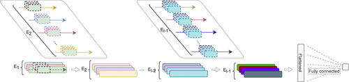
CNN A convolutional neural network using the ReLU activation function, with architecture illustrated in Figure 1. Note that this architecture is slightly more flexible than the one considered in Section 2.2, hence, we expect it to perform at least as well in terms of approximation rate. Both for the potential outcome model μ₀ and the propensity score p, the number of channels in the input layer is one. For the outcome models 128 channels in the first hidden layer and 16 channels in the second hidden layer have been used, while 32 channels in the first hidden layer and 8 channels in the second hidden layer have been used for fitting the propensity score. We have implemented the CNN together with AIPW estimation strategy in the package DNNcausal which is available at https://github.com/stat4reg/DNNcausal.

Fig. 1 Illustration of the convolutional neural network used in the simulations and the real data study. Each layer, $i\in \{0,\dots ,l\}$ contains different number of channels E_i, where E₀ (not shown in the figure) is the number of time series in the set of input covariates. Each channel (feature map) in a given layer is formed by first applying $E_{i-1}$ number of kernels (convolution filters) on the vectors in layer i–1 and then summing the results. There exist some covariates which are not time series. Inclusion of those vectors in the neural network is not illustrated in the figure for simplification purpose. A fully connected feed-forward structure has been used for those covariates and the results are then combined with the results from the time-series data in the flattening layer demonstrated above.

MLP A Rectified Linear Unit activation function based feedforward neural network with two hidden layers. Two different feedforward architectures are used in order to estimate μ₀, and p (propensity score). The networks for fitting the outcome model consist of 128 and 80 nodes within the two layers, respectively. For the propensity score, two layers contain 32 and 8 nodes, respectively.post-lasso Nuisance models are fitted in two steps, where all higher order terms up to order three are considered. First, a lasso variable selection step is performed using the R-package hdm (Chernozhukov, Hansen, and Spindler 2016), and then maximum likelihood is used to fit the models with the selected covariates (those with coefficients not shrinked to zero by lasso). The lasso penalty parameter is selected as $\lambda =2.2\sqrt{n}{\Phi }^{-1}([\log \hspace{0.17em}(n)-0.1]{[2p\hspace{0.17em}\log \hspace{0.17em}(n)]}^{-1})$ (Belloni et al. 2012). Variable selection is performed using two different strategies: double selection which takes the union of variables selected by regressing outcome and treatment variables and uses that to refit both models (Belloni, Chernozhukov, and Hansen 2014; Moosavi, Häggström, and de Luna 2021), and single selection, which uses two sets of variables selected by regressing outcome and treatment, and refits each of the models using their corresponding set (Farrell 2015).

We use the above nuisance function estimators in several different estimators of τ_t, as follows:

AIPW is implemented using CNN, MLP, and post-lasso with both single and double selection (denoted respectively: DRcnn, DRmlp, DRss, DRds).

OR estimator with post-lasso and double selection (denoted ORds).

TMLE using the R-package tmle and the function SL.nnet to fit all nuisance functions (denoted TMLE).

Full details with code and description of choice of architectures and hyperparameter for this simulation study are available in the Supplementary Materials.

We set sample sizes to n = 5000 and $10,000$, and run 1000 replicates. Bias, standard errors (both estimated and Monte Carlo), mean squared errors (MSE, bias squared plus variance) and empirical coverages for 95% confidence intervals are reported in Table 1 and 2.

Table 1 Setting 1 DGP: Bias, standard errors (both estimated, Est sd, and Monte Carlo, MC sd), MSEs and empirical coverages for 95% confidence intervals over 1000 replicates.

	bias	coverage	MC sd	Est sd	MSE
n = 5000
DRcnn	0.185	0.947	1.379	1.366	1.935
DRmlp	0.426	0.940	1.353	1.331	2.013
ORds	0.001	0.947	1.404	1.392	1.970
DRss	0.002	0.948	1.404	1.395	1.971
DRds	0.003	0.948	1.404	1.395	1.972
tmle	0.044	0.944	1.396	1.384	1.951
n = 10, 000
DRcnn	0.089	0.958	0.971	0.972	0.951
DRmlp	0.223	0.949	0.961	0.958	0.973
ORds	0.001	0.955	0.981	0.982	0.962
DRss	0.001	0.955	0.981	0.984	0.962
DRds	0.001	0.955	0.981	0.984	0.962
tmle	0.028	0.957	0.981	0.978	0.963

Table 2 Setting 2 DGP: Bias, standard errors (both estimated and Monte Carlo), MSEs and empirical coverages for 95% confidence intervals over 1000 replicates.

	bias	coverage	MC sd	Est sd	MSE
n = 5000
DRcnn	0.047	0.937	0.094	0.101	0.011
DRmlp	0.076	0.890	0.095	0.099	0.015
ORds	0.233	0.206	0.083	0.085	0.061
DRss	0.233	0.260	0.083	0.092	0.061
DRds	0.235	0.250	0.083	0.092	0.062
tmle	0.233	0.204	0.083	0.085	0.061
n = 10, 000
DRcnn	0.025	0.945	0.070	0.072	0.006
DRmlp	0.036	0.928	0.070	0.072	0.006
ORds	0.224	0.040	0.062	0.061	0.054
DRss	0.224	0.054	0.062	0.065	0.054
DRds	0.226	0.045	0.061	0.065	0.055
tmle	0.224	0.041	0.062	0.061	0.054

We first comment the results for the settings with normally distributed errors for the outcome models. The DGP of Setting 1 (Table 1) is the least complex one and its polynomial form is favorable to the post-lasso methods which are based on higher order terms. It is therefore expected that the post-lasso methods ORds, DRss, DRds have low bias. DRcnn has larger bias, but decreasing with n. All methods have similar MSEs even though DRcnn has the lowest MSE for the largest sample size. Empirical coverages are close to the nominal 95% level for all methods.

The DGP of Setting 2 (Table 2) is less smooth and we observe that the DRcnn and DRmlp methods have the lowest biases and MSEs, where DRcnn performs slightly better. TMLE and post-lasso both have such a large bias that the confidence interval coverages are far from being at the nominal level. It should be noted, however, that the TMLE uses the built-in feedforward neural network, which is not adjusted to the generated datasets, and so the comparison is not a fair one between TMLE and the DR estimators.

Results for the heavy-tailed Gamma errors are available in the supplementary materials.

The latter results are similar to those above, although Lasso approaches perform slightly worse while neural networks perform slightly better.

4 Effect of Early Retirement on Health

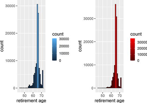
The existing theoretical and empirical evidence on the effects of early retirement on health are mixed, and both positive and negative results may be expected and have been reported in different situations; see Barban et al. (2020) and the references therein. In this context, we add to the empirical evidence by studying the effect of early retirement on health using a database linking at the individual level a collection of socio-economic and health registers on the whole Swedish population (Lindgren et al. 2016). This allows us to follow until 2017 two complete cohorts born in 1946 and 1947 and residing in Sweden in 1990. As health outcome we observe the number of days in hospital per year after retirement. To study the effects of early retirement we consider those who were still alive at age 62, and either retire at age 62 (T = 1, treatment) or retire later (T = 0, control group). For the cohorts studied, retirement pensions are accessible from age 61, although the usual age of retirement is 65 years of age (see Figure 2 for descriptive statistics on age of retirement). Therefore, retiring at age of 62 is considered as early retirement since it decreases your annual pension transfers compared to later retirement; see, for example, Barban et al. (2020) for details on the Swedish pension system. Barban et al. (2020) also contains a study on the effects of early retirement, although based on fewer measurements for time-dependent covariates and using a matching design. This study provides new evidence by taking into account richer histories of the time-dependent covariates, and by incorporating CNN to address complex dynamics in pretreatment confounding covariates.

Fig. 2 Retirement age for men and women who belong to the cohorts born in Sweden 1946 and 1947. The last staple in each histogram displays those who retired at age 71 or later.

More precisely, the design of the study is as follows. An individual alive at age 62 is considered as taking early retirement at that age if her/his pension transfers become larger than income from work at that age for the first time (i.e., they were never so earlier). For replicability, the exact definition using income and transfer variables from the Swedish registers are available in the supplementary materials. The health outcomes of interest are the number of hospitalization days per year during the next five years following early retirement. We, however, check first whether early retirement has an effect on survival during the five first years following early retirement. There were no (or hardly significant) such effects at the 5% level (results reported in the appendix, Table 4) and we therefore focus the analysis on the survivors when looking at effects on hospitalization. The following covariates are used as input in the CNN architures to fit treatment and outcome nuisance models. Besides the birth year we include the the following (pretreatment) covariates measured at 61 years of age: marriage status, municipality, education level, Spouse education level, and the number of biological children. Moreover, we consider the measurements of the following covariates for each of the 10 years preceding retirement: days of hospitalization and open health care, annual income from labor, annual income from pension, annual income from unemployment, annual income from early retirement and sickness benefit, annual compensation for illness, and spouse retirement status. Thus, covariates include eight time(-structured) series of 10 observations each per individual. We do separate analyses for men and women which gives two samples of approximately 100,000 individuals each.

Table 4 Effect of early retirement on survival (binary outcomes death = 1), during five years of follow up for the early retirees, and 95% confidence intervals.

	Women n = 106,916		Men n = 105,149
The first year after treatment is considered for the outcome
naive	0.002		–0.001
DRcnn	0.005	(0.002, 0.008)	–0.001	(–0.005, 0.003)
DRmlp	0.004	(0.000, 0.007)	–0.003	(–0.013, 0.007)
ORds	0.003	(–0.194, 0.200)	0.000	(–0.150, 0.151)
DRss	0.003	(0.000, 0.006)	0.000	(–0.002, 0.003)
DRds	0.003	(0.000, 0.007)	0.000	(–0.002, 0.003)
tmle	0.003	(0.000, 0.006)	0.000	(–0.002, 0.003)
The second year after treatment is considered for the outcome
naive	0.002		–0.002
DRcnn	0.007	(0.003, 0.012)	0.001	(–0.005, 0.007)
DRmlp	0.006	(0.002, 0.011)	0.001	(–0.003, 0.006)
ORds	0.005	(–0.164, 0.174)	0.002	(–0.130, 0.133)
DRss	0.005	(0.001, 0.009)	0.002	(–0.002, 0.005)
DRds	0.005	(0.001, 0.009)	0.002	(–0.002, 0.005)
tmle	0.005	(0.001, 0.009)	0.002	(–0.002, 0.005)
The third year after treatment is considered for the outcome
naive	0.000		–0.002
DRcnn	–0.052	(–0.166, 0.063)	0.005	(0.000, 0.010)
DRmlp	0.004	(–0.001, 0.009)	0.008	(0.003, 0.013)
ORds	0.004	(–0.150, 0.159)	0.004	(–0.114, 0.122)
DRss	0.005	(0.000, 0.009)	0.004	(–0.000, 0.009)
DRds	0.005	(0.001, 0.010)	0.005	(0.000, 0.009)
tmle	0.005	(0.000, 0.009)	0.004	(–0.000, 0.009)
The fourth year after treatment is considered for the outcome
naive	–0.003		& -0.006
DRcnn	0.002	(–0.005, 0.008)	–0.001	(–0.007, 0.005)
DRmlp	0.001	(–0.005, 0.006)	0.005	(–0.000, 0.011)
ORds	0.003	(–0.140, 0.145)	0.002	(–0.107, 0.110)
DRss	0.003	(–0.002, 0.008)	0.002	(–0.003, 0.007)
DRds	0.004	(–0.001, 0.009)	0.002	(–0.003, 0.007)
tmle	0.003	(–0.002, 0.008)	0.002	(–0.003, 0.007)
The fifth year after treatment is considered for the outcome
naive	–0.005		–0.007
DRcnn	0.002	(–0.004, 0.009)	0.001	(–0.006, 0.008)
DRmlp	0.009	(0.002, 0.016)	0.009	(0.002, 0.016)
ORds	0.001	(–0.131, 0.134)	0.002	(–0.098, 0.102)
DRss	0.002	(–0.004, 0.008)	0.002	(–0.003, 0.008)
DRds	0.003	(–0.003, 0.008)	0.003	(–0.003, 0.009)
tmle	0.002	(–0.004, 0.008)	0.002	(–0.003, 0.008)

The code giving details on the CNN architectures and tuning parameters can be found in the supplementary materials. We also apply the other methods evaluated in the simulation study above.

Results are presented in Table 3. Based on the naive estimation not controlling for confounders, early retirement has a clear positive effect on health (varying between 0.167 and 0.396 average number of days) and for the five years of follow up considered. These naive effects are larger for women in the beginning. These negative effects disappear when controlling for the considered covariates. This is seen most clearly with CNN which yields the effects smaller than 0.1 day (in absolute value) for all cases but one. Confidence intervals at the 95% level cover zero in most cases. Thus, while there appeared to be a positive effect on health of early retirement, this effect was probably due to confounding.

Table 3 Effect of early retirement on number of days in hospital during five years of follow up, for the early retirees, and 95% confidence intervals.

	Women		Men
The first year	n = 106,437		n = 104,459
naive	–0.396		–0.167
DRcnn	0.062	(–0.060, 0.183)	–0.037	(–0.256, 0.183)
DRmlp	–0.062	(–0.192, 0.069)	0.138	(–0.079, 0.355)
ORds	–0.135	(–0.231, –0.039)	0.018	(–0.156, 0.192)
DRss	–0.138	(–0.232, –0.045)	0.025	(–0.148, 0.199)
DRds	–0.128	(–0.222, –0.035)	0.028	(–0.145, 0.202)
tmle	–0.143	(–0.237, –0.049)	0.018	(–0.156, 0.192)
The second year	n = 105,776		n = 103,560
naive	–0.354		–0.192
DRcnn	–0.082	(–0.231, 0.067)	0.122	(–0.042, 0.285)
DRmlp	–0.083	(–0.224, 0.058)	0.214	(0.041, 0.387)
ORds	–0.104	(–0.215, 0.007)	–0.007	(–0.161, 0.146)
DRss	–0.098	(–0.207, 0.011)	0.011	(–0.142, 0.164)
DRds	–0.081	(–0.190, 0.027)	0.014	(–0.139, 0.167)
tmle	–0.111	(–0.220, –0.002)	0.011	(–0.142, 0.163)
The third year	n = 105,039		n = 102,547
naive	–0.277		–0.173
DRcnn	0.011	(–0.153, 0.175)	0.030	(–0.140, 0.200)
DRmlp	0.200	(0.029, 0.370)	1.094	(–0.894, 3.083)
ORds	–0.034	(–0.192, 0.124)	0.014	(–0.136, 0.165)
DRss	–0.018	(–0.174, 0.138)	0.024	(–0.126, 0.175)
DRds	–0.010	(–0.167, 0.146)	0.027	(–0.123, 0.178)
tmle	–0.018	(–0.174, 0.139)	0.027	(–0.123, 0.178)
The fourth year	n = 104,293		n = 101,502
naive	–0.179		–0.216
DRcnn	0.067	(–0.181, 0.315)	0.085	(–0.082, 0.252)
DRmlp	0.804	(–0.432, 2.040)	–0.517	(–1.723, 0.688)
ORds	0.032	(–0.186, 0.250)	–0.032	(–0.194, 0.131)
DRss	0.042	(–0.176, 0.259)	–0.016	(–0.178, 0.146)
DRds	0.056	(–0.162, 0.273)	–0.008	(–0.170, 0.154)
tmle	0.033	(–0.185, 0.251)	–0.015	(–0.177, 0.147)
The fifth year	n = 103,477		n = 100,325
naive	–0.232		–0.230
DRcnn	–0.012	(–0.185, 0.161)	–0.095	(–0.276, 0.085)
DRmlp	–0.979	(–2.982, 1.024)	–0.153	(–0.443, 0.138)
ORds	–0.019	(–0.169, 0.132)	–0.050	(–0.195, 0.095)
DRss	–0.013	(–0.163, 0.137)	–0.035	(–0.179, 0.109)
DRds	0.000	(–0.150, 0.151)	–0.029	(–0.173, 0.116)
tmle	–0.014	(–0.164, 0.136)	–0.034	(–0.178, 0.110)

5 Discussion

We have proposed and studied a semiparametric estimation strategy for average causal effects which combine convolutional neural network with AIPW. As long as the conditions given are met, this strategy yields locally efficient and uniformly valid inference. The use of CNN has the advantage over fully-connected feed forward neural networks that they are more efficient on the number of weights (free parameters) used for approximating the nuisance functions, and are geared to take into account time invariant local features (LeCun and Bengio 1995) in confounding time series variables. If no time series or other structured confounding is available in the data, then other machine learning algorithms may be as appropriate to use to fit nuisance functions.

A main contribution of the article is to show under which conditions CNN fits of nuisance functions achieve $n^{-1/4}$ convergence rate required to obtain uniformly valid inference on an ACE. Using the result in Farrell, Liang, and Misra (2021) in which convergence rate of a ReLU-based feed-forward network is shown to follow (1), we show that the rate conditions in Assumption 3 are fulfilled. Specifically, we use CNN with a given complexity for which we show that approximation rate in (1) is small enough. A key component of result in Farrell, Liang, and Misra (2021) is the upper bound on empirical process terms found in Bartlett, Bousquet, and Mendelson (2005) based on Rademacher averages, which are measures of function space complexity. Global Rademacher averages do not provide fast rates as in (1). To derive this fast rate, localization analysis is employed which takes into consideration only intersection of the function space with a ball around the goal function; considering that in reality the algorithm only searches in a neighborhood around the true function. Moreover, the tight bound on Pseudo-dimension of deep nets found in Bartlett et al. (2019) is used.

We also present numerical experiments showing the performance of the estimation strategy in finite sample and compare it to other machine learning based estimation strategies. The applicability of the method is illustrated through a population wide observational study of the effect of early retirement on hospitalization in Sweden.

Supplementary Materials

Supplementary materials are available on-line at https://github.com/stat4reg/Causal_CNN if nothing else stated.

R-package for DRcnn and DRmlp estimators:The R-package DNNcausal implements estimators of average causal effect and average causal effect on the treated, combining AIPW with deep neural networks fits of nuisance functions described in the article; available at https://github.com/stat4reg/DNNcausal. (GNU zipped tar file)

Simulation description: Code used for the simulations in Section 3. (.md file)

Simulations results: Results of simulations, and a description of how hyperparameters are tuned. (.md file)

Case study description: Supplementary material on the design of the study of the effects of early retirement on health reported in Section 4. (.md file)

Acknowledgments

We are grateful to Xijia Liu and Jenny Häggström for helpful comments that have improved the article. We acknowledge funding from the Swedish Research Council and the Marianne and Marcus Wallenberg Foundation. The Umeå SIMSAM Lab data infrastructure used in this study was developed with support from the Swedish Research Council, the Riksbanken Jubileumsfond and by strategic funds from Umeå University.

Disclosure Statement

The authors report there are no competing interests to declare.

Appendix

In this section we also consider the Sobolev space $H^{\beta }(\Omega )$ that is defined using the L² norm instead of the $L^{\infty }$ norm. Moreover, let ${\Vert f\Vert }_{L^2(\Omega )}$ be the L² norm of a function f defined on Ω.

A.1 Proof of Theorem 2

Proof.

Let $\Omega ={[-1,1]}^d$. For any α that satisfies $\left|\alpha \right|\le \beta$, by Hölder’s inequality, we have: $${\Vert D^{\alpha }f\Vert }_{L^2(\Omega )}\le 2^{d/2}{\Vert D^{\alpha }f\Vert }_{L^{\infty }(\Omega )}.$$

Therefore, $f\in H^{\beta }(\Omega )$ and $${\Vert f\Vert }_{H^{\beta }(\Omega )}=\sqrt{\sum _{\alpha ,\left|\alpha \right|\le \beta }{\Vert D^{\alpha }f\Vert }_{L^2(\Omega )}^2}\le \sqrt{\sum _{\alpha ,\left|\alpha \right|\le \beta }{2}^d}\le \sqrt{n_{\beta }}{2}^{d/2}$$hold by ${\max }_{\stackrel{\alpha ,\left|\alpha \right|\le \beta }{}}{\Vert D^{\alpha }f\Vert }_{L^{\infty }(\Omega )}\le 1$, where $n_{\beta }=\#\{\alpha ,|\alpha |\le \beta \}$. Moreover, Ω has a Lipschitz domain interior and measure zero boundary. Therefore, by Sobolev extension theorem (Stein 1970, Theorem 5) there is an extension $F\in H^{\beta }({\mathbb{R}}^d)$ of f for which $${\Vert F\Vert }_{H^{\beta }({\mathbb{R}}^d)}\le C{\Vert f\Vert }_{H^{\beta }(\Omega )}\le C\sqrt{n_{\beta }}{2}^{d/2},$$ where $n_{\beta }$ is a constant that depends on β and C is a constant independent of β.

Let $v_{F,2}:={\int }_{{\mathbb{R}}^d}{\Vert \omega \Vert }_1^2|\widehat{F}(\omega )|d\omega$, where $\widehat{F}(\omega )$ is the Fourier transform of F. $v_{F,2}$ is finite since ${\Vert F\Vert }_{H^{\beta }({\mathbb{R}}^d)}={\Vert {(1+|\omega {|}^2)}^{\beta /2}\widehat{F}(\omega )\Vert }_{L^2}$ (see Theorem 7 chapter 5.8.4 in Evans (2010); Characterization of H^k by Fourier transform), and ${\int }_{{\mathbb{R}}^d}{\Vert \omega \Vert }_1^2|\widehat{F}(\omega )|d\omega \le {\Vert {(1+|\omega {|}^2)}^{\beta /2}\widehat{F}(\omega )\Vert }_{L^2}·{\Vert \left|\right|\omega |{|}_1^2{(1+|\omega {|}^2)}^{-\beta /2}\Vert }_{L^2}$ by Cauchy–Schwarz inequality. Consequently, $v_{F,2}\le \left|\right|F\left|\right|·c_{d,\beta }$, where $c_{d,\beta }$ is ${\Vert \left|\right|\omega |{|}_1^2{(1+|\omega {|}^2)}^{-\beta /2}\Vert }_{L^2}$ and it is finite due to the assumption $\beta >\frac{d}{2}+2$.

Since $F\in H^{\beta }({\mathbb{R}}^d)$ and using Theorem 2 in Klusowski and Barron (2018) we have: $${\Vert F-F_m\Vert }_{C(\Omega )}\le c_0{v}_{F,2}\max \{\sqrt{\hspace{0.17em}\log \hspace{0.17em}m},\sqrt{d}\}{m}^{-\frac{1}{2}-\frac{1}{d}},$$where $m=E\lfloor \frac{(s-1)L}{d}-1\rfloor ,F_m(x)={\beta }_0+{\alpha }_{0}x+\frac{v}{m}{\sum }_{k=1}^m{\beta }_k{({\alpha }_k·x-t_k)}_{+},$ ${\beta }_k\in [-1,1]$, ${\Vert {\alpha }_k\Vert }_1=1,t_k\in [0,1],{\beta }_0=F(0)$, ${\alpha }_0=\nabla F(0),{(x)}_{+}$ is $\max (0,x)$ (ReLU).

Let $F_m^i:=\frac{1}{E}{\beta }_0+\frac{1}{E}{\alpha }_{0}x+\frac{v}{m}{\sum }_{k=im+1}^{(i+1)m}{\beta }_k{({\alpha }_{k}x-t_k)}_{+}$. It is shown in Zhou (2020), using $s\ge 2$ and $L\ge 2d/(s-1)$, that $F_m^i{|}_{\Omega }$ belongs to the following function space $${\mathcal{C}}_L^{w,b}=\left\{\sum _{k=1}^{d_L}{c}_k{h}_k^{(L)}(x):c\in {\mathbb{R}}^{d_L}\right\}.$$

Therefore, by the definition of $\mathcal{C}$, we can directly conclude that $F_m{|}_{\Omega }$ belongs to $\mathcal{C}$. Let $f_{L,E}^{w,b}:=F_m{|}_{\Omega }$. Then, we have (A.1) $$\begin{array}{cc}{\Vert f-f_{L,E}^{w,b}\Vert }_{C(\Omega )}\hfill & ={\Vert F-F_m\Vert }_{C(\Omega )}\hfill \\ \hfill & \le c_0{v}_{F,2}\max \{\sqrt{\hspace{0.17em}\log \hspace{0.17em}m},\sqrt{d}\}{m}^{-\frac{1}{2}-\frac{1}{d}}\hfill \\ \hfill & \le c_0{c}_{d,\beta }{\Vert F\Vert }_{H^{\beta }({\mathbb{R}}^d)}\max \{\sqrt{\hspace{0.17em}\log \hspace{0.17em}m},\sqrt{d}\}{m}^{-\frac{1}{2}-\frac{1}{d}}.\hfill \end{array}$$(A.1)

The final result is obtained from the facts that $\frac{1}{2}(s-1)LE\le md\le (s-1)LE,s\ge 2$ and $\beta >2+d/2$ ($c_{d,\beta }$ is bounded). □

A.2 Proof of Theorem 3

Proof.

The rate conditions (a) and (b) of Assumption 3 are fulfilled if both ${\mathbb{E}}_n[{({\widehat{\mu }}_t(x_i)-{\mu }_t(x_i))}^2]$ and ${\mathbb{E}}_n[{(\widehat{p}(x_i)-p(x_i))}^2]$ are $o_P(n^{-1/2})$. For this, the three terms in the upper bound (5) in Theorem 1 must be $o_P(n^{-1/2})$. For the first term, based on 2, we have $$\begin{array}{c}\frac{QL\hspace{0.17em}\log \hspace{0.17em}Q}{n}\log \hspace{0.17em}n\asymp \frac{E{L}^3\hspace{0.17em}\log \hspace{0.17em}(E{L}^2)}{n}\log \hspace{0.17em}n\asymp \frac{{\hspace{0.17em}\log \hspace{0.17em}}^6(n)\hspace{0.17em}\log \hspace{0.17em}\left(n^{\frac{d+1}{2d+4}}{\hspace{0.17em}\log \hspace{0.17em}}^{4}n\right)}{n^{\frac{2d+5}{4d+8}}}\\ \hspace{0.17em}\log \hspace{0.17em}n=o_P(n^{-1/2}).\end{array}$$

The second term is also $o_P(n^{-1/2})$ if $\gamma =o(n^{1/2})$. For the third term, using Theorem 2 we have $${\epsilon }_{\mathcal{W},\mathcal{C}}\le \frac{\sqrt{\frac{2d+1}{4d+8}\log \hspace{0.17em}n+\hspace{0.17em}\log \hspace{0.17em}{\hspace{0.17em}\log \hspace{0.17em}}^{2}n}}{n^{\frac{2d+1}{8d}}{\hspace{0.17em}\log \hspace{0.17em}}^{\frac{d+2}{d}}n}.$$

To prove condition (c) of Assumption 3, we use the proof of lemma Farrell, Liang, and Misra (2021, Lemma 10). In this proof it is shown that for an arbitrary class of feedforward neural networks with probability at least $1-\hspace{0.17em}\exp \hspace{0.17em}(-n^{\frac{d+3}{4d+8}}{\hspace{0.17em}\log \hspace{0.17em}}^{6}n)$ $$\begin{array}{cc}\hfill & {\mathbb{E}}_n[({\widehat{\mu }}_{t,\mathcal{C}}(x_i)-{\mu }_t(x_i))(1-\frac{\mathbb{1}\{t_i=t\}}{\mathbb{P}[T=t|X=x_i]}\left)\right]\hfill \\ \hfill & \le C(\frac{QL\hspace{0.17em}\log \hspace{0.17em}Q}{n}\log \hspace{0.17em}n+\frac{\hspace{0.17em}\log \hspace{0.17em}\hspace{0.17em}\log \hspace{0.17em}n+n^{\frac{d+3}{4d+8}}{\hspace{0.17em}\log \hspace{0.17em}}^{6}n}{n}+{\epsilon }_{\mathcal{W},\mathcal{C}}^2).\hfill \end{array}$$

Therefore, we can conclude that under the stated conditions $$\begin{array}{cc}\hfill & {\mathbb{E}}_n[({\widehat{\mu }}_t(x_i)-{\mu }_t(x_i))(1-\frac{\mathbb{1}\{t_i=t\}}{\mathbb{P}[T=t|X=x_i]}\left)\right]\hfill \\ \hfill & \le C{\mathbb{E}}_n\left[{({\widehat{\mu }}_t(x_i)-{\mu }_t(x_i))}^2\right]=o_P(n^{-1/2}).\hfill \end{array}$$

□

A.3 Early Retirement Effects on Survival

Additional results on the effect of early retirement on survival can be found in Table 4.

References

- Barban, N., de Luna, X., Lundholm, E., Svensson, I., and Billari, F. C. (2020), “Causal Effects of the Timing of Life-Course Events: Age at Retirement and Subsequent Health,” Sociological Methods & Research, 49, 216–249. DOI: 10.1177/0049124117729697.
- Bartlett, P. L., Bousquet, O., and Mendelson, S. (2005), “Local Rademacher Complexities,” The Annals of Statistics, 33, 1497–1537. DOI: 10.1214/009053605000000282.
- Bartlett, P. L., Harvey, N., Liaw, C., and Mehrabian, A. (2019), “Nearly-Tight vc-Dimension and Pseudodimension Bounds for Piecewise Linear Neural Networks,” The Journal of Machine Learning Research, 20, 2285–2301.
- Belloni, A., Chen, D., Chernozhukov, V., and Hansen, C. (2012), “Sparse Models and Methods for Optimal Instruments with an Application to Eminent Domain,” Econometrica, 80, 2369–2429.
- Belloni, A., Chernozhukov, V., and Hansen, C. (2014), “Inference on Treatment Effects After Selection Among High-Dimensional Controls,” The Review of Economic Studies, 81, 608–650. DOI: 10.1093/restud/rdt044.
- Chen, X., and White, H. (1999), “Improved Rates and Asymptotic Normality for Nonparametric Neural Network Estimators,” IEEE Transactions on Information Theory, 45, 682–691. DOI: 10.1109/18.749011.
- Chernozhukov, V., Chetverikov, D., Demirer, M., Duflo, E., Hansen, C., Newey, W., and Robins, J. (2018), “Double/Debiased Machine Learning for Treatment and Structural Parameters,” The Econometrics Journal, 21, C1–C68. DOI: 10.1111/ectj.12097.
- Chernozhukov, V., Hansen, C., and Spindler, M. (2016), “hdm: High-Dimensional Metrics,” R Journal, 8, 185–199. DOI: 10.32614/RJ-2016-040.
- Evans, L. C. (2010), Partial Differential Equations, Providence, RI: American Mathematical Society.
- Farrell, M. H. (2015), “Robust Inference on Average Treatment Effects with Possibly More Covariates than Observations,” Journal of Econometrics, 189, 1–23. DOI: 10.1016/j.jeconom.2015.06.017.
- Farrell, M. H. (2018), “Robust Inference on Average Treatment Effects with Possibly more Covariates than Observations,” arXiv:1309.4686v3.
- Farrell, M. H., Liang, T., and Misra, S. (2021), “Deep Neural Networks for Estimation and Inference,” Econometrica, 89, 181–213. DOI: 10.3982/ECTA16901.
- Kennedy, E. H. (2016), “Semiparametric Theory and Empirical Processes in Causal Inference,” in Statistical Causal Inferences and their Applications in Public Health Research, eds. H. He, P. Wu, D.-G. Chen, pp. 141–167, Cham: Springer.
- Klusowski, J. M., and Barron, A. R. (2018), “Approximation by Combinations of Relu and Squared Relu Ridge Functions with l1 and l0 Controls,” IEEE Transactions on Information Theory, 64, 7649–7656.
- LeCun, Y., and Bengio, Y. (1995), “Convolutional Networks for Images, Speech, and Time Series,” in The Handbook of Brain Theory and Neural Networks, 3361, ed. M. A. Arbib, pp. 255–258, Cambridge, MA: MIT Press.
- Lindgren, U., Nilsson, K., de Luna, X., and Ivarsson, A. (2016), “Data Resource Profile: Swedish Microdata Research from Childhood into Lifelong Health and Welfare (Umeå SIMSAM Lab),” International Journal of Epidemiology, 45, 1075–1075. DOI: 10.1093/ije/dyv358.
- Moosavi, N., Häggström, J., and de Luna, X. (2021), “The Costs and Benefits of Uniformly Valid Causal Inference with High-Dimensional Nuisance Parameters,” Statistical Science, to appear ArXiv preprint arXiv:2105.02071.
- Robins, J. M., Rotnitzky, A., and Zhao, L. P. (1994), “Estimation of Regression Coefficients When Some Regressors are not Always Observed,” Journal of the American statistical Association, 89, 846–866. DOI: 10.1080/01621459.1994.10476818.
- Rubin, D. B. (1974), “Estimating Causal Effects of Treatments in Randomized and Nonrandomized Studies,” Journal of Educational Psychology, 66, 688–701. DOI: 10.1037/h0037350.
- Scharfstein, D., Rotnitzky, A., and Robins, J. (1999), “Rejoinder to Comments on “Adjusting for Non-ignorable Drop-Out Using Semiparametric Non-response Models?” Journal of the American Statistical Association, 94, 1121–1146. DOI: 10.2307/2669930.
- Stein, E. M. (1970), Singular Integrals and Differentiability Properties of Functions (PMS-30), Princeton: Princeton University Press.
- Tan, Z. (2007), “Comment: Understanding OR, PS and DR,” Statistical Science, 22, 560–568. DOI: 10.1214/07-STS227A.
- Tsiatis, A. (2006), Semiparametric Theory and Missing Data, New York: Springer.
- van der Laan, M., and Rose, S. (2011), Targeted Learning: Causal Inference for Observational and Experimental Data. Springer Series in Statistics, New York: Springer.
- Zhou, D.-X. (2020), “Universality of Deep Convolutional Neural Networks,” Applied and Computational Harmonic Analysis, 48, 787–794. DOI: 10.1016/j.acha.2019.06.004.