Smooth and Probabilistic PARAFAC Model with Auxiliary Covariates

Abstract

As immunological and clinical studies become more complex, there is an increasing need to analyze temporal immunophenotypes alongside demographic and clinical covariates, where each subject receives matrix-valued time series observations for potentially high-dimensional longitudinal features, as well as other static characterizations. Researchers aim to find the low-dimensional embedding of subjects using matrix-valued time series observations and investigate relationships between static clinical responses and the embedding. However, constructing these embeddings can be challenging due to high dimensionality, sparsity, and irregularity in sample collection over time. In addition, the incorporation of static auxiliary covariates is frequently desired during such a construction. To address these issues, we propose a smoothed probabilistic PARAFAC model with covariates (SPACO) that uses auxiliary covariates of interest. We provide extensive simulations to test different aspects of SPACO and demonstrate its application to an immunological dataset from patients with SARS-CoV-2 infection. Supplementary materials for this article are available online.

KEYWORDS:

• Missing data
• Probabilistic model
• Tensor decomposition
• Time series

1 Introduction

Sparsely observed multivariate time series data are now common in immunological studies. For each subject or participant $i$ $(i=1,\dots ,I)$, we can collect multiple measurements on $J$ features over time, but often at $n_i$ different time stamps $\{t_{i,1},\dots ,t_{i,n_i}\}$. For example, for each subject, immune profiles are measured for hundreds of markers at irregular sampling times in Lucas et al. (2020) and Rendeiro et al. (2021). Let $X_i\in {\mathbb{R}}^{n_i\times J}$ be the longitudinal measurements for subject $i$, and $\mathit{X}\in {\mathbb{R}}^{I\times T\times J}$ be the sparse three-way tensor collecting $X_i$ for all $I$ subjects, where $T$ is the number of unique time points across all subjects, for example, $T=\left|{\cup }_i\right\{t_{i,1},\dots ,t_{i,n_i}\left\}\right|$. 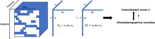A major computational task in practice is to construct low-dimensional embeddings that capture data variability in $\mathit{X}$ across subjects. Tensor decomposition is a widely used technique for achieving this goal. Figure 1 demonstrates the PARAFAC/CP tensor decomposition and utilization of the decomposition results (Harshman and Lundy 1994), where we approximate a tensor by the sum of rank-one tensors. Apart from tensor reconstruction and denoising, the decomposition of the three-way tensor X provides decomposed factors $U$, $V$, and $\Phi$, which aim to capture major variations along the subject, feature, and time directions, respectively. These factors can be used for further downstream analysis. For instance, factors $U$ (also denoted as the subject scores) serve as the aforementioned subject embeddings, which can be used to investigate the relationship between immune profiles and various clinical/demographic covariates.

Fig. 1 Illustration of the PARAFAC/CP decomposition method for immunoprofiles measured longitudinally. The white color represents missing data in the time direction. The three-way tensor is approximated as the sum of $K$ rank-one tensors $F^1,\dots ,F^K$. Each rank-one tensor $F^k$ $(k=1,\dots ,K)$ can be expressed using a factor along the subject direction $(U_k)$, a factor along the feature direction $(V_k)$, and a factor along the time direction $({\Phi }_k)$. The factors associated with the tensor decomposition can be used in downstream analysis.

The immune profiles are usually highly sparse observed along the time dimensions, that is, the sets {$t_{i,1},\dots ,t_{i,n_i}$} for different subjects i tend to be small in size and have low overlaps, resulting in a high missing rate along the time dimension of X (Figure 1). In addition, researchers may have access to nontemporal covariates for each subject, such as medical conditions and demographic information, which may partially explain the variation in the temporal measurements of X across subjects. As an example, the IMPACT study (Lucas et al. 2020) analyzed immune profiles of 98 COVID-19 infected individuals. Researchers measured immune profiles for more than 30 days after symptom onset, but only an average of 1.84 measured time points per subject. Auxiliary demographic information, including sex and age, and several preexisting medical conditions, were also collected. To better estimate $U$ in this example, a tensor decomposition tool that can properly model the longitudinal behavior of the factors and incorporate available auxiliary covariates is needed.

In this article, we propose SPACO (smooth and probabilistic PARAFAC model with auxiliary covariates) to adapt to the sparsity long the time dimension in X and use the auxiliary covariates Z. SPACO assumes that X is a noisy realization of some low-rank signal tensor whose time components are smooth and subject scores have a potential dependence on the auxiliary covariates Z: $$\begin{array}{c}{x}_{\mathit{itj}}=\sum _{k=1}^K{u}_{ik}{\varphi }_{tk}{v}_{jk}+{ϵ}_{\mathit{itj}},\hspace{1em}{ϵ}_{\mathit{itj}}\sim \mathcal{N}(0,{\sigma }_j^2)\\ {\mathit{u}}_i={(u_{ik})}_{k=1}^K\sim \mathcal{N}({\mathit{\eta }}_i,{\Lambda }_f),\hspace{1em}{\mathit{\eta }}_i={\beta }^{\top }{\mathbf{z}}_i.\end{array}$$

Here, (a) z_i is the ith row of Z and $\beta \in {\mathbb{R}}^{q\times K}$ describes the dependence of the expected subject score for subject i on z_i, (b) u_ik, ${\varphi }_{tk}$, v_jk are the subject score, trajectory value and feature loading for factor k in the PARAFAC model and the observation indexed by (i, t, j) where ${\mathit{u}}_i$ has a normal prior $\mathcal{N}({\mathit{\eta }}_i,{\Lambda }_f)$. We impose smoothness on time trajectories ${({\varphi }_{tk})}_{t=1}^{\top }$ and sparsity on β to deal with the irregular sampling along the time dimension and potentially high dimensionality in Z.

Alongside the proposal of the model, we will delve into several issues pertinent to SPACO, including model initialization, auto-tuning of smoothness and sparsity in β, and hypothesis testing on β. Effectively addressing these concerns is crucial for applying SPACO in practice. In the remainder of the article, we summarize work closely related to our study in Section 1.1. We describe the SPACO model in Section 2 and discuss model parameter estimation with predetermined tuning parameters in Section 3. Section 4 is dedicated to the examination of the aforementioned issues that bear practical significance. A comparative analysis of SPACO with existing methods on synthetic data is presented in Section 5. Lastly, in Section 6, we employ SPACO on a highly sparse tensor containing immunological measurements from SARS-COV-2 infected patients. We also provide a Python package, SPACO, for researchers who are interested in using the proposed method.

1.1 Related Work

Matrix-valued observations have become increasingly important in modern applications, particularly in the context of dimension reduction or matrix-valued data clustering (Chang 1983; Vichi, Rocci, and Kiers 2007; Viroli 2011; Anderlucci and Viroli 2015).

Tensor decomposition is a useful technique for modeling matrix-valued observations, and has been applied in various fields (Acar and Yener 2008; Kolda and Bader 2009; Sidiropoulos et al. 2017). In the study of multivariate longitudinal data, researchers in economics have combined tensor decomposition with auto-cross-covariance estimation and autoregressive models (Fan, Fan, and Lv 2008; Lam, Yao, and Bathia 2011; Fan, Liao, and Mincheva 2011; Bai and Wang 2015, 2016; Wang, Liu, and Chen 2019; Wang et al. 2021). However, these approaches are either not compatible with highly sparse data or do not scale well with the feature dimensions, both of which are important for medical applications.

Functional PCA (Besse and Ramsay 1986; Yao, Müller, and Wang 2005) is often used for modeling sparse longitudinal data in the matrix form. It uses the smoothness of time trajectories to handle sparsity in longitudinal observations and estimates the eigenvectors and factor scores under this smoothness assumption. Yokota, Zhao, and Cichocki (2016) and Imaizumi and Hayashi (2017) introduced smoothness into tensor decomposition and estimated the parameters by iteratively solving penalized regression problems. However, these methods do not consider auxiliary covariates.

It has been previously discussed that including auxiliary information could potentially improve our estimation. For example, Li, Shen, and Huang (2016) proposed the supervised sparse and functional principal component (SupSFPC) method and observed that auxiliary covariates improve signal estimation quality in the matrix setting for modeling multivariate longitudinal observations. In Chen, Tsay, and Chen (2020), the authors observed that inclusion of auxiliary constraints improve the quality of tensor decomposition. Lock and Li (2018) proposed SupCP, a supervised multiway factorization model with complete observation that employs a probabilistic tensor model (Tipping and Bishop 1999; Mnih and Salakhutdinov 2007; Hinrich and Mørup 2019). Although an extension to sparse tensor is straightforward, SupCP does not model smoothness and can be highly affected by severe missingness along the time dimension.

To address these limitations, we propose SPACO, an extension of functional PCA and SupSFPC to the setting of three-way tensor decomposition using the parallel factor (PARAFAC) model (Carroll, Pruzansky, and Kruskal 1980; Harshman and Lundy 1994). SPACO jointly models smooth longitudinal data with potentially high-dimensional static covariates Z using a probabilistic model. When Z is unavailable, we refer to the SPACO model as SPACO-. SPACO- itself is also an attractive alternative to existing tensor decomposition implementations with probabilistic modeling, smoothness regularization, and automatic parameter tuning. In our numerical experiments, we demonstrate the advantages of SPACO and SPACO- over several state-of-the-art tensor decomposition methods and the improvement of SPACO over SPACO- by using Z.

2 SPACO Model

2.1 Notations

We use (a) bolded uppercase letters to represent three-way tensors, (b) regular uppercase letters to represent a matrix, and (c) bolded lowercase to represent vectors. Following this convection, let $\mathit{X}\in {\mathbb{R}}^{I\times T\times J}$ be the tensor for some sparse multivariate longitudinal observations, where I is the number of subjects, J is the number of features, and T is the number of total unique time points. Let $X_I:=(\begin{array}{ccc}{\mathit{X}}_{:,:,1}& \dots & {\mathit{X}}_{:,:,J}\end{array})\in {\mathbb{R}}^{I\times (TJ)},X_T:=(\begin{array}{ccc}{\mathit{X}}_{:,:,1}^{\top }& \dots & {\mathit{X}}_{:,:,J}^{\top }\end{array})\in {\mathbb{R}}^{T\times (IJ)},X_J:=(\begin{array}{ccc}{\mathit{X}}_{:,1,:}^{\top }& \dots & {\mathit{X}}_{:,T,:}^{\top }\end{array})\in {\mathbb{R}}^{J\times (IT)}$ be the matrix unfolding of X in the subject/feature/time dimension respectively. For any matrix A, we let $A_{i:}/A_{:i}$ denote its ith row/column, and often write $A_{:i}$ as A_i for the ith column for convenience. We also define:

Tensor product $⊚$: $\mathit{a}\in {\mathbb{R}}^I,\mathit{b}\in {\mathbb{R}}^T,\mathit{c}\in {\mathbb{R}}^J$, then, $\mathit{A}=\mathit{a}⊚\mathit{b}⊚\mathit{c}\in {\mathbb{R}}^{I\times T\times J}$ with ${\mathit{A}}_{\mathit{itj}}={\mathit{a}}_i{\mathit{b}}_t{\mathbf{c}}_j$.

Kronecker product ⊗: $A\in {\mathbb{R}}^{I_1\times K_1},B\in {\mathbb{R}}^{I_2\times K_2}$, then $C=A\otimes B\in {\mathbb{R}}^{(I_1{I}_2)\times (K_1{K}_2)}$ is the Kronecker product of A and B: $C=A\otimes B=(\begin{array}{ccc}{A}_{11}B\hfill & \dots \hfill & A_{1K_1}B\hfill \\ ⋮\hfill & \ddots \hfill & ⋮\hfill \\ A_{I_{1}1}B\hfill & \dots \hfill & A_{I_1{K}_1}B\hfill \end{array})\in {\mathbb{R}}^{(I_1{I}_2)\times (K_1{K}_2)}$.

Column-wise Khatri-Rao product $\odot$: $A\in {\mathbb{R}}^{I_1\times K},B\in {\mathbb{R}}^{I_2\times K}$, then $C=A\odot B\in {\mathbb{R}}^{(I_1{I}_2)\times K}$ with $C_{:,k}=(A_{:,k}\otimes B_{:,k})$ for $k=1,\dots ,K$.

Element-wise multiplication $·$: $A,B\in {\mathbb{R}}^{I\times K}$, then $C=A·B\in {\mathbb{R}}^{I\times K}$ with $C_{ik}=(A_{ik}{B}_{ik})$; for $\mathit{b}\in {\mathbb{R}}^K,C=A·\mathit{b}=A\text{diag}\{{\mathit{b}}_1,\dots ,{\mathit{b}}_K\}$; for $\mathit{b}\in {\mathbb{R}}^I,C=\mathit{b}·A=\text{diag}\{{\mathit{b}}_1,\dots ,{\mathit{b}}_I\}A$.

2.2 Smooth and Probabilistic PARAFAC Model with Covariates

We assume X to be a noisy realization of an underlying signal array F which is a rank K tensor with $U/\Phi /V$ be the decomposed factor matrices, for example, $\mathbf{F}={\sum }_{k=1}^K{U}_k⊚{\Phi }_k⊚V_k$, where $U_k/{\Phi }_k/V_k$ are kth columns of $U/\Phi /V$. We denote the rows of $U/\Phi /V$ by ${\mathit{u}}_i/{\mathit{\varphi }}_t/{\mathit{v}}_j$, and their entries by $u_{ik}/{\varphi }_{tk}/v_{jk}$. We let x_itj denote the (i, t, j)-entry of X. Then, (1) $$x_{\mathit{itj}}=\sum _{k=1}^K{u}_{ik}{\varphi }_{tk}{v}_{jk}+{\epsilon }_{\mathit{itj}},{\mathit{u}}_i\sim \mathcal{N}({\mathit{\eta }}_i,{\Lambda }_f),{\epsilon }_{\mathit{ijt}}\sim \mathcal{N}(0,{\sigma }_j^2),$$(1) where ${\Lambda }_f=\text{diag}\{s_1^2,\dots ,s_K^2\}$ is a K × K diagonal covariance matrix and ${\mathit{\eta }}_i$ is a mean vector of length K. In practice, although the observation tensor X is almost always of high-rank, it is often assumed that F is (or approximately) low-rank with K being small.

We set ${\mathit{\eta }}_i=\mathbf{0}$ in the absence of auxiliary covariates $Z\in {\mathbb{R}}^{I\times q}$. In the setting where we are interested in explaining the heterogeneity ${\mathit{\eta }}_i$ across subjects using Z, we may model ${\mathit{\eta }}_i$ as a function of ${\mathbf{z}}_i:=Z_{i,:}$. Here, we consider a linear model ${\eta }_{ik}={\mathbf{z}}_i^{\top }{\beta }_k$ for $k=1,\dots ,K$, where η_ik is the kth entry of ${\mathit{\eta }}_i$ and $\beta \in {\mathbb{R}}^{q\times K}$ is the coefficients matrix describing the dependence of subject scores on Z. To avoid confusion, we will always call X the “features”, and Z the “covariates” or “variables”.

Recalling that $X_I\in {\mathbb{R}}^{I\times (TJ)}$ is the unfolding of X in the subject direction, we write $\overrightarrow{i}$ for the indices of observed values in the ith row of X_I, and $X_{I,\overrightarrow{i}}$ for the vector of these observed values. Each such observed value x_itj has noise variance ${\sigma }_j^2$, and we write ${\Lambda }_{\overrightarrow{i}}$ to represent the diagonal covariance matrix with diagonal values ${\sigma }_j^2$ being the corresponding variances for ${\epsilon }_{\mathit{ijt}}$ at indices in $\overrightarrow{i}$. Similarly, we define $\{\overrightarrow{t},X_{T,\overrightarrow{t}},{\Lambda }_{\overrightarrow{t}}\}$ for the unfolding $X_T\in {\mathbb{R}}^{T\times (IJ)}$, and $\{\overrightarrow{j},X_{J,\overrightarrow{j}},{\Lambda }_{\overrightarrow{j}}\}$ for the observed indices, the associated observed vector and diagonal covariance matrix for the jth row in $X_J\in {\mathbb{R}}^{J\times (IT)}$. We set $\Theta =\{V,\Phi ,\beta ,({\sigma }_j^2,j=1,\dots ,J),(s_k^2,k=1,\dots ,K)\}$ to denote all model parameters. Set $H=V\odot \Phi \in {\mathbb{R}}^{(TJ)\times K}$ and ${\mathbf{f}}_i=X_{I,\overrightarrow{i}}-H_{\overrightarrow{i},:}{\mathit{\eta }}_i$ as the residual vector after removing mean signals from observations for subject i. If U is observed, the complete log-likelihood is (2) $$\begin{array}{c}L(\mathit{X},U|\Theta )=-\frac{1}{2}\sum _i({\mathbf{f}}_i^{\top }{\Lambda }_{\overrightarrow{i}}^{-1}{\mathbf{f}}_i+{({\mathit{u}}_i-{\mathit{\eta }}_i)}^{\top }{\Lambda }_f^{-1}({\mathit{u}}_i-{\mathit{\eta }}_i)\\ +\hspace{0.17em}\log \hspace{0.17em}\left|{\Lambda }_{\overrightarrow{i}}\right|+I\hspace{0.17em}\log \hspace{0.17em}\left|{\Lambda }_f\right|).\end{array}$$(2)

Set ${\tilde{\Sigma }}_i={\Lambda }_{\overrightarrow{i}}+H_{\overrightarrow{i}}{\Lambda }_f{H}_{\overrightarrow{i}}^{\top }$. The marginalized log-likelihood integrating out the randomness in U enjoys a closed form (Lock and Li 2018): (3) $$L(\mathit{X}|\Theta )\propto -\frac{1}{2}\left(\sum _i{\mathbf{f}}_i^{\top }{\tilde{\Sigma }}_i^{-1}{\mathbf{f}}_i+\hspace{0.17em}\log \hspace{0.17em}\left|{\tilde{\Sigma }}_i\right|\right).$$(3)

Model parameters in (3) are not identifiable due to (a) parameters rescaling from $({\Phi }_k,V_k,{\beta }_k,s_k^2)$ to $(c_1{\Phi }_k,c_2{V}_k,c_3{\beta }_k,c_3^2{s}_k^2)$ for any $c_1{c}_2{c}_3=1$, and (b) reordering of different component k for $k=1,\dots ,K$. More discussions of the model identifiability can be found in Lock and Li (2018). Hence, adopting similar rules from Lock and Li (2018), we require

(C.1) $⏧V_k{⏧}_2^2=1,⏧{\Phi }_k{⏧}_2^2=T$.

(C.2)The latent components are in decreasing order based on their overall variances ${\Lambda }_{f,kk}+⏧Z{\beta }_k{⏧}_2^2/I$, and the first nonzero entries in V_k and ${\Phi }_k$ to be positive, for example, $v_{k1}>0$ and ${\varphi }_{k1}>0$ if they are nonzero.

In the immunological application being considered, U represents subject scores, which are latent variables characterizing differences across subjects, V represents feature loadings, revealing the composition of factors using the original features and aiding downstream interpretation, and $\Phi$ represents time trajectories interpreted as function values sampled from some underlying smooth functions ${\varphi }_k(t)$ at a set of discrete-time points where the sampling in the time direction is often highly sparse.

Algorithm 1:

SPACO with fixed penalties

Data: X, Ω, λ₁, λ₂, K

Result: Estimated V, $\Phi$, β, s², ${\sigma }^2$ and posterior distribution of $U|\Theta ,\mathit{X}$ and the marginalized density $\mathbf{P}(\mathit{X}|\Theta )$.

1. Initialization of V, $\Phi$, β, s², ${\sigma }^2$ and the posterior distribution of U;

2. while Not converged do

3. for $k=1,\dots ,K$ do

4. ${\beta }_k\leftarrow \arg {\min }_{{\beta }_k}\{-L(\mathit{X}|\Theta )+{\lambda }_{2k}\left|{\beta }_k\right|\}$

5. $V_k\leftarrow \arg {\min }_{V_k}\left[J(\Theta ;{\Theta }_0)+{\nu }_V⏧V_k{⏧}_2^2\right]$, ν_V is the largest value leading to the minimizer having $⏧V_k{⏧}_2^2=1$

6. ${\Phi }_k\leftarrow \arg {\min }_{{\Phi }_k}\left[J(\Theta ;{\Theta }_0)+{\nu }_{\Phi }⏧{\Phi }_k{⏧}_2^2\right],{\nu }_{\Phi }$ is the largest value leading to the minimizer having $⏧{\Phi }_k{⏧}_2^2=T$

7. $s_k^2\leftarrow \arg {\max }_{s_k^2}{\mathbb{E}}_{U|{\Theta }_0}L(\mathit{X},U|\Theta )$.

8. end

9. For $j=1,\dots ,J$: ${\sigma }_j^2\leftarrow \arg {\max }_{{\sigma }_j^2}{\mathbb{E}}_{U|{\Theta }_0}L(\mathit{X},U|\Theta )$.

10. Update the posterior distribution (posterior mean and covariance) of U.

11. end

We address the challenge of sparse sampling utilizing the smoothness assumption in ${\varphi }_k(t)$ and encourage it by directly penalizing the function values via a penalty term $\sum _k{\lambda }_{1k}{\Phi }_k^{\top }\Omega {\Phi }_k$. This article considers a Laplacian smoothing (Sorkine et al. 2004) with a weighted adjacency matrix Γ. Let $\mathcal{T}[t]$ be the time associated with the tth slice along the time dimension, for example, time associated with ${\mathit{X}}_{.,t.,}$. We define Ω and Γ as $$\begin{array}{c}\Omega ={\Gamma }^{\top }\Gamma ,\\ \Gamma =\left(\mathrm{}\mathrm{}\begin{array}{ccccc}\frac{1}{\mathcal{T}\left[2\right]-\mathcal{T}\left[1\right]}\hfill & -\frac{1}{\mathcal{T}\left[2\right]-\mathcal{T}\left[1\right]}\hfill & \dots \hfill & 0\hfill & 0\hfill \\ 0\hfill & \frac{1}{\mathcal{T}\left[3\right]-\mathcal{T}\left[2\right]}\hfill & \ddots \hfill & 0\hfill & ⋮\hfill \\ ⋮\hfill & ⋮\hfill & \ddots \hfill & ⋮\hfill & ⋮\hfill \\ 0\hfill & 0\hfill & \dots \hfill & \frac{1}{\mathcal{T}\left[T\right]-\mathcal{T}[T-1]}\hfill & -\frac{1}{\mathcal{T}\left[T\right]-\mathcal{T}[T-1]}\hfill \end{array}\mathrm{}\mathrm{}\right)\\ \in {\mathbb{R}}^{T\times (T-1)}.\end{array}$$

The Laplacian smoothing discourages abrupt trajectory changes in observations from close-by time points, which is usually a reasonable assumption biologically. Practitioners may choose other forms for Ω based on their applications. For example, if practitioners want ${\varphi }_k(t)$ to have slowly varying derivatives, they can also use a penalty matrix that penalizes changes in gradients over time.

Further, when the number of covariates q in Z is moderately large, we may wish to impose sparsity in the β parameter. We encourage such sparsity by including a lasso penalty (Tibshirani 2011) in the model. In summary, our goal is then to find parameters maximizing the expected penalized log-likelihood, or minimizing the penalized expected deviance loss $J(\Theta )$, under norm constraints: (4) $$\begin{array}{c}\min J(\Theta ):=-\frac{1}{2}L(\mathit{X}|\Theta )+\sum _{k=1}^K{\lambda }_{1k}{\Phi }_k^{\top }\Omega {\Phi }_k+\sum _k{\lambda }_{2k}|{\beta }_k|\\ \hspace{1em}\mathrm{s}.\mathrm{t}\hspace{1em}⏧{\mathrm{V}}_{\mathrm{k}}{⏧}_2^2\text{=1},⏧{\Phi }_{\mathrm{k}}{⏧}_2^2\text{=T},\text{ for all }k=1,\dots ,K.\end{array}$$(4)

The objective only incorporates the identifiability constraint (C.1). By changing the signs in V, $\Phi$, β and reordering them, we can always ensure (C.2) without altering the attained objective value.

Equation (4)(4) $$\begin{array}{c}\min J(\Theta ):=-\frac{1}{2}L(\mathit{X}|\Theta )+\sum _{k=1}^K{\lambda }_{1k}{\Phi }_k^{\top }\Omega {\Phi }_k+\sum _k{\lambda }_{2k}|{\beta }_k|\\ \hspace{1em}\mathrm{s}.\mathrm{t}\hspace{1em}⏧{\mathrm{V}}_{\mathrm{k}}{⏧}_2^2\text{=1},⏧{\Phi }_{\mathrm{k}}{⏧}_2^2\text{=T},\text{ for all }k=1,\dots ,K.\end{array}$$(4) characterizes a nonconvex problem. We will obtain local optimal solutions via an alternating update procedure: (a) we update β through lasso regressions while keeping other parameters fixed, (b) we update other model parameters using the EM algorithm while keeping β fixed. See Section 3 for more details.

3 Model Parameter Estimation

Given the model rank K and penalty terms ${\lambda }_{1k},{\lambda }_{2k}$, we alternately update parameters β, V, U, s², and ${\sigma }^2$ with a mixed EM procedure described in Algorithm 1. We briefly explain the updating steps here:

1. Given other parameters, we find β to directly minimize the objective by solving a least-squares regression problem with lasso penalty.

2. Fixing β, we update the other parameters using an EM procedure. Denote the current parameters as ${\Theta }_0$. At the M-step, we minimize the penalized expected negative log-likelihood

   $\begin{array}{c}\hspace{1em}J(\Theta ;{\Theta }_0)\\ :={\mathbb{E}}_{\mathit{U}|{\Theta }_0}\left\{-L(\mathit{X},U|\Theta )+\sum _k{\lambda }_{1k}{\Phi }_k^{\top }\Omega {\Phi }_k+\sum _k{\lambda }_{2k}|{\beta }_k|\right\},\end{array}$ (5)

   under the current posterior distribution $U|{\Theta }_0,\mathit{X}$. We adopt a block-wise parameter updating scheme where we update V_k, ${\Phi }_k$, Λ_f and ${\sigma }_j^2$ sequentially.

Algorithm 1 describes the high level ideas of our updating schemes. The posterior distribution of ${\mathit{u}}_i$ for each row in U is Gaussian, with posterior covariance Σ_i and posterior mean ${\mathit{\mu }}_i$ given below, (6) $${\Sigma }_i={(H_{\overrightarrow{i}}^{\top }{\Lambda }_{\overrightarrow{i}}^{-1}{H}_{\overrightarrow{i}}+{\Lambda }_f^{-1})}^{-1}$$(6) (7) $${\mathit{\mu }}_i={\Sigma }_i\left({\Lambda }_f^{-1}{\beta }^{\top }{\mathbf{z}}_i+H_{\overrightarrow{i}}^{\top }{\Lambda }_{\overrightarrow{i}}^{-1}{X}_{I,\overrightarrow{i}}\right).$$(7)

In line 5 and 6, we guarantee the norm constraints on V_k and ${\Phi }_k$ by adding an additional quadratic term and set the coefficient ν to guarantee the norm requirements. Although the problem is not convex, our proposed approaches yield optimal solutions for updating different parameter blocks in the sub-routines, and the penalized (marginalized) deviance loss is nonincreasing over the iterations.

Theorem 3.1.

In Algorithm 1, let ${\Theta }_{\mathcal{l}}$ and ${\Theta }_{\mathcal{l}+1}$ are the estimated parameters at the beginning and end of the $\mathcal{l}$th iteration of the outer while loop. We have $J({\Theta }^{\mathcal{l}})\ge J({\Theta }^{\mathcal{l}+1})$.

Proof of Theorem 3.1 is given in Appendix B.1. Derivations and explicit steps for carrying subroutines are deferred to Appendix A.1.

Algorithm 2:

Initialization of SPACO

1. Let $V_{\perp }$ be the top K₃ left singular vectors of X_J using only the observed columns.

2. Set $Y(k)=(Y_1(k),\dots ,Y_T(k))\in {\mathbb{R}}^{I\times T}$, where $Y_t(k)={\mathit{X}}_{:,t,:}{(V_{\perp })}_k\in {\mathbb{R}}^I$.

3. Let ${\Phi }_{\perp }$ be the top K₂ eigenvectors from functional PCA on the row aggregation of matrices Y(k) $k=1,\dots ,K_3$. (see Appendix A.2 for details on functional PCA.)

4. Let $\tilde{U}=\arg {\min }_U\{⏧X_I-U{(V_{\perp }\otimes {\Phi }_{\perp })}^{\top }{⏧}_F^2+\delta ⏧U{⏧}_F^2\}\in {\mathbb{R}}^{I\times K^2}$, where δ is a small regularization parameter to avoid severe over-fitting to the noise.

5. Let $U_{\perp }$ be the top K left singular eigenvectors of $\tilde{U}$, and $\tilde{G}=U_{\perp }^{\top }\tilde{U}\in {\mathbb{R}}^{K\times K^2}$. Let $\mathit{G}\in {\mathbb{R}}^{K\times K\times K}$ be the estimated core array from rearranging $\tilde{G}$.

6. Let ${\sum }_{k=1}^K{A}_k⊚B_k⊚C_k$ be the rank-K CP approximation of G. Stack these as the columns of $A,B,C\in {\mathbb{R}}^{K\times K}$, and set $[U,\Phi ,V]=[U_{\perp }A,{\Phi }_{\perp }B,V_{\perp }C]$.

7. For each $k=1,\dots ,K$, rescale the initializers to satisfy constraints on V and $\Phi$

4 Initialization, Tuning and Testing

4.1 Initialization

One popular initialization approach for PARAFAC decomposition is through the Tucker decomposition $[U_{\perp },{\Phi }_{\perp },V_{\perp };\mathit{G}]$ of X using HOSVD/MLSVD (De Lathauwer, De Moor, and Vandewalle 2000) where $\mathit{G}\in {\mathbb{R}}^{K_1\times K_2\times K_3}$ is the core tensor and $U_{\perp }\in {\mathbb{R}}^{I\times K_1},{\Phi }_{\perp }\in {\mathbb{R}}^{T\times K_2},V_{\perp }\in {\mathbb{R}}^{J\times K_3}$ are unitary matrices multiplied with the core tensors along the subject, time and feature directions respectively ($K_1\text{/}{K}_2\text{/}{K}_3$ is the smallest between K and $I\text{/}T\text{/}J$), and then perform PARAFAC decomposition on the small core tensor G (Bro and Andersson 1998; Phan, Tichavskỳ, and Cichocki 2013). Here, we propose to initialize SPACO with Algorithm 2, which combines the aforementioned approach with functional PCA (Yao, Müller, and Wang 2005) to handle sparse longitudinal data. Algorithm 2 proceeds as follows: (a) perform SVD on X_J to get $V_{\perp }$; (b) project X_J onto each column of $V_{\perp }$ and perform functional PCA to estimate ${\Phi }_{\perp }$; (c) a ridge-penalized regression regressing rows of X_I on $V_{\perp }\otimes {\Phi }_{\perp }$, and estimate $U_{\perp }$ and G from the regression coefficients.

In a noiseless model with δ = 0 and complete temporal observations, one may replace the functional PCA step of Algorithm 2 with standard PCA. Then $[U,\Phi ,V]$ becomes a PARAFAC decomposition of $\frac{1}{1+\delta }\mathit{X}$.

Lemma 4.1.

Suppose $\mathit{X}={\sum }_{k=1}^K{U}_k^{*}⊚{\Phi }_k^{*}⊚V_k^{*}$ and is completely observed. Replace ${\Phi }_{\perp }$ in Algorithm 2 by the top K eigenvectors of $W=\frac{1}{I}{\sum }_{k=1}^{K}Y{(k)}^{\top }Y(k)$. Then, the outputs $U,\Phi ,V$ of Algorithm 2 satisfy that $\mathit{X}=(1+\delta ){\sum }_{k=1}^K{U}_k⊚{\Phi }_k⊚V_k$.

By default, we set $\delta =\frac{1}{\sqrt{J\times T}}$. Proof of Lemma 4.1 is given in Appendix B.2.

4.2 Auto-Selection of Tuning Parameters

Selection of regularizers λ₁ and λ₂: One possible approach to select the tuning parameters ${\lambda }_{1k}$ and ${\lambda }_{2k}$ is through cross-validation. However, this can be computationally expensive even when tuning each parameter sequentially. Additionally, determining a suitable set of candidate values for the parameters before running the SPACO algorithm can be challenging. To address these issues, we adopt nested cross-validation, which has been empirically demonstrated to be useful (Huang, Shen, and Buja 2008; Li, Shen, and Huang 2016). Specifically, we tune the parameters within their corresponding subroutines as follows:

1. In the update for ${\Phi }_k$, we conduct column-wise leave-one-out cross-validation to select ${\lambda }_{1k}$, where all observations from a single time point are left out (See Appendix A.3.)

2. In the update for β_k, we perform K-fold cross-validation to select ${\lambda }_{2k}$.

Rank selection: Rank selection can be performed through cross-validation, as suggested in SupCP (Lock and Li 2018). To reduce computational costs, we adopt two strategies (see Appendix A.4 for more details):

1. We initialize the cross-validation parameters with estimates obtained from running a full SPACO/SPACO- analysis and only carry out a limited number of iterations to update the parameters. We find that using 5 or 10 iterations is sufficient in our experiments (the default maximum number of iterations is 10).

Algorithm 3:

Randomization test for Z_j

1 for $k=1,\dots ,K$ do

3 Construct responses and features as described in Lemma 4.2.

5 Define ${\widehat{\beta }}_k$ by $${\widehat{\beta }}_k=\arg \underset{{\beta }_k:{\beta }_{k,j}=0}{\min }\left\{\sum _{i=1}^I\frac{1}{w_i}{({\mathbf{z}}_i^{\top }{\beta }_k-{\tilde{y}}_i)}^2+{\lambda }_{2k}|{\beta }_k{|}_1\right\}.$$

7 Compute the designed test statistic T using $(Z_j,Z_{j^c},\tilde{\mathbf{y}},{\widehat{\beta }}_{j^c,k})$.

9 Compute randomized statistics ${\underset{¯}{T}}^b$ using $({\underset{¯}{Z}}_j^b,Z_{j^c},\tilde{\mathbf{y}},{\widehat{\beta }}_{j^c,k})$, where ${\underset{¯}{Z}}_j^b$ for $b=1,\dots ,B$ are (conditionally or marginally) independent copies of Z_j.

11 Let $\widehat{G}(.)$ be the empirical estimate of the CDF of T under H₀ using $\{{\underset{¯}{T}}_1,\dots ,{\underset{¯}{T}}^B,T\}$, and return the two-sided p-value $p=[1-\widehat{G}(\left|T\right|)]+\widehat{G}(-|T|)$.

12 end

2. We start the analysis with the smallest possible rank and gradually increase it. We terminate the analysis when either the cross-validated marginal log-likelihood stops improving or when we reach the maximum rank that we are willing to consider.

4.3 Covariate Importance

In Section 5 of our synthetic experiments, we found that incorporating Z could improve the estimation of subject scores when Z strongly influenced the subject scores. This leads us to question how to determine the significance of such covariates when they are present. Here, we consider the construction of approximated p-values from partial independence/marginal independence tests between Z_j and η_k: $$H_{0k}^{\text{partial}}:Z_j\perp \text{}\perp {\eta }_k|Z_{j^c},\mathrm{\hspace{1em}}\mathrm{\hspace{1em}}{H}_{0k}^{\text{margin}}:Z_j\perp \text{}\perp {\eta }_k,$$both of which are practical interest.

Recap on randomization-based hypothesis testing: Before introducing our proposal, we will revisit concepts of hypothesis testing via randomization in the traditional setting where we investigate the relationship between a response variable y and a covariate variable z.

First, we investigate the marginal independence between y and z, with the null hypothesis $H_0^{\text{margin}}:z\perp \text{}\perp y$. The randomization test, widely employed for independence testing, offers a valid p-value without assuming a specific dependence structure between y and z (Fisher 1936; Pitman 1937; Efron et al. 2001; Ernst 2004). Here, we outline the randomization test for marginal independence. Let $t(\mathbf{z},\mathbf{y})$ be a test statistic where $\mathbf{z}$ and $\mathbf{y}$ are the observation vectors for z and response y. For instance, one may set $t(\mathbf{z},\mathbf{y})=|\text{cor}(\mathbf{z},\mathbf{y})|$. Let $T:=t(\mathbf{z},\mathbf{y})$ and ${\underset{¯}{T}}_b:=t({\underset{¯}{\mathbf{z}}}^b,\mathbf{y})$, for $b=1,\dots ,B$, where ${\underset{¯}{\mathbf{z}}}^b$ is either a permutation of $\mathbf{z}$ or a vector of independent realizations from the marginal distribution of z. There are subtle differences between using ${\underset{¯}{\mathbf{z}}}^b$ generated from a permutation and using one generated from the marginal distribution (Onghena 2017); however, we will not distinguish them in this context. Under the null hypothesis $H_0^{\text{margin}},T,{\underset{¯}{T}}_1,\dots ,{\underset{¯}{T}}_B$ are exchangeable. Thus, for any $\alpha \in (0,1)$, we have $P(T>t_{1-\alpha }^{*}|\mathbf{y})\le \alpha$, where $t_{1-\alpha }^{*}$ is the $(1-\alpha )$-percentile of the empirical distribution constituted by $(T,{\underset{¯}{T}}_1,\dots ,{\underset{¯}{T}}_B)$.

In addition to marginal independence, many statistical inquiries focus on the conditional or partial independence between y and z given additional variable(s) z_o, with the null hypothesis $H_0^{\text{partial}}:z\perp \text{}\perp y|z_o$. For illustration, one may consider a linear regression model expressed by the following equation: $$y=z\beta +z_o^{\top }\gamma +\zeta ,$$where ζ is a mean-zero noise term independent of z and z_o. In recent years, the conditional randomization test has emerged as a popular method for testing the partial independence between variables z and y, given z_o. If the conditional distribution of $z|z_o$ is known, the conditional randomization test generates new copies of z from the distribution $z|z_o$, allowing the construction of randomized test statistics that are exchangeable with the original one under $H_0^{\text{partial}}$. This approach leverages the known conditional distribution to construct valid testing procedures without imposing additional constraints on the relationship between y and $(z,z_o)$ (Candes et al. 2018; Berrett et al. 2020). To be specific, we define the test statistic $t(\mathbf{z},{\mathbf{z}}_o,\mathbf{y})$ where z_o represents the observations for variables z_o. The test statistics $t(\mathbf{z},{\mathbf{z}}_o,\mathbf{y})$ can take any function form, for example, we can set $t(\mathbf{z},{\mathbf{z}}_o,\mathbf{y})=|\text{cor}(\mathbf{z},\mathbf{y})|$. Let $T:=t(\mathbf{z},{\mathbf{z}}_o,\mathbf{y})$ and ${\underset{¯}{T}}_b:=t({\underset{¯}{\mathbf{z}}}^b,{\mathbf{z}}_o,\mathbf{y})$, where ${\underset{¯}{\mathbf{z}}}^b$ is an independent copy of the observation vector generated from the distribution of $z|z_o$, for $b=1,\dots ,B$. Under the null hypothesis $H_0^{\text{partial}}$, the test statistics T and ${\underset{¯}{T}}^b$ have the same conditional distribution given ${\mathbf{z}}_o$ and $\mathbf{y}$. Hence, $P(T>t_{1-\alpha }^{*}|{\mathbf{z}}_o,\mathbf{y})\le \alpha$, where $t_{1-\alpha }^{*}$ is the $(1-\alpha )$-percentile of the conditional distribution of $(T,{\underset{¯}{T}}_1,\dots ,{\underset{¯}{T}}_B)$ (Candes et al. 2018).

In this article, we propose to adapt the idea of randomization tests to construct robust p-values for testing independence/conditional independence between factors and auxiliary covariates in SPACO, where the responses are not given beforehand.

Oracle randomization test in SPACO: Returning to SPACO, we first consider the ideal scenario where V, $\Phi$, s², and ${\sigma }^2$ are given. Lemma 4.2 forms the basis of our proposal.

Lemma 4.2.

Given $V,\Phi ,s^2,{\sigma }^2$, and let ${\beta }_{\mathcal{l}}^{*}$ be the true regression coefficients on the covariates Z for ${\mu }_{\mathcal{l}},\mathcal{l}=1,\dots ,K$. For any $k=1,\dots ,K$, set $${\underset{¯}{\Sigma }}_i={\left({(V\odot \Phi )}_{\overrightarrow{i}}^{\top }{\Lambda }_{\overrightarrow{i}}{(V\odot \Phi )}_{\overrightarrow{i}}\right)}^{-1},$$ $$w_i=s_k^2+{\left({\underset{¯}{\Sigma }}_i\right)}_{kk},$$ $$y_i={\left({\underset{¯}{\Sigma }}_i\right)}_{k,:}{H}_{\overrightarrow{i},:}^{\top }{\Lambda }_{\overrightarrow{i}}{X}_{I,\overrightarrow{i}}.$$

Then, we have $y_i={\mathbf{z}}_i^{\top }{\beta }_k^{*}+{\xi }_i$, where ${\xi }_i\sim \mathcal{N}(0,w_i)$ is independent of auxiliary covariates.

Lemma 4.2 is proved via direct calculation in Appendix B.3. Readers may recognize that y and Z match the regression model, potentially allowing the application of the standard randomization technique. Proposition 4.3 details our construction of both observed and randomized test statistics, the validity of which is a result of Lemma 4.2 and Lemma F.1 in Candes et al. (2018). A proof is provided in Appendix B.4 for completeness.

Proposition 4.3.

Set $T_{\text{partial}}=\frac{\sum _i\frac{1}{w_i}(y_i-Z_{i,j^c}^{\top }{\beta }_{j^c,k})Z_{ij}}{\sum _i\frac{1}{w_i}{Z}_{ij}^2}$ for ${\beta }_{j^c,k}$ estimated without the jth covariate Z_j, $T_{\text{margin}}=\frac{\sum _i\frac{1}{w_i}{y}_i{Z}_{ij}}{\sum _i\frac{1}{w_i}{Z}_{ij}^2}$. Replacing Z_j with the properly randomized ${\underset{¯}{Z}}_j$ to create ${\underset{¯}{T}}_{\text{margin}}$ and ${\underset{¯}{T}}_{\text{partial}}$, where ${\underset{¯}{Z}}_j$ is a permutation of Z_j for ${\underset{¯}{T}}_{\text{margin}}$ and ${\underset{¯}{Z}}_j$ is independently generated from $Z_j|Z_{j^c}$ for ${\underset{¯}{T}}_{\text{partial}}$, we have (8) $$T_{\text{margin}}\left|\tilde{\mathbf{y}}\stackrel{d}{=}{\underset{¯}{T}}_{\text{margin}}\right|\mathbf{y},\mathrm{\hspace{1em}}\mathrm{\hspace{1em}}\text{ under }{H}_{0k}^{\text{margin}},$$(8) (9) $$T_{\text{partial}}|(\mathbf{y},Z_{j^c})\stackrel{d}{=}{\underset{¯}{T}}_{\text{partial}}|(\mathbf{y},Z_{j^c}),\mathrm{\hspace{1em}}\mathrm{\hspace{1em}}\text{ under }{H}_{0k}^{\text{partial}}.$$(9)

Algorithm 3 outlines our proposal. The conditional randomization test involves generating ${\underset{¯}{Z}}_j$ from the conditional distribution $Z_j|Z_{j^c}$, which is estimated using an appropriate exponential family distribution. Further details on the generations of ${\underset{¯}{Z}}_j$ can be found in Appendix A.5.

Approximated p-value construction with estimated model paramters: The true model parameters V, $\Phi$, s², and ${\sigma }^2$ are unknown, so we will substitute the true parameters with their empirical estimates. However, the empirical estimates from a full SPACO fit tend to suffer from fitting toward the noise. To mitigate such influence, we use $V,\Phi$ from cross-validation described in Section 4.2. Specifically, for $i\in {\mathcal{V}}_m$, the index set for fold m, we construct ${\tilde{y}}_i$ using estimates $V^{-m},{\Phi }^{-m}$ and the prior covariance estimate ${\Lambda }_f^{-m}$ from other folds, by setting ${\tilde{y}}_i={({\underset{¯}{\Sigma }}_i)}_{k,:}{(V^{-m}\odot {\Phi }^{-m})}^{\top }{\Lambda }_{\overrightarrow{i}}{X}_{I,\overrightarrow{i}}$ with ${\underset{¯}{\Sigma }}_i$ is also estimated using $V^{-m}$, ${\Phi }^{-m}$, and ${\Lambda }_f^{-m}$. This procedure, referred to as cross-fit, employs data from other folds to estimate certain parameters, and forms the final quantity of interest with them and data from current fold. Additionally, initializing each fold at the global solution enhances the comparability of the constructed $\tilde{y}$ and $\tilde{z}$ across different folds. This cross-fit approach yields improved Type I error control compared to the naive incorporation of full estimates in our empirical experiments.

5 Numerical Studies with Synthetic Data

This section presents an evaluation of SPACO using synthetic Gaussian data. The noise variance is fixed at 1, and the true rank is set to K = 3. The simulated data consists of $(\mathit{X},Z)$ with dimensions $(I,T,J,q)\in \{(100,30,10,100),(100,30,500,100)\}$. The observed rate (i.e., $1-$ the missing rate) along the time dimension is set to $r\in \{100\%,50\%,10\%\}$, with observed time stamps chosen randomly for each subject. To generate the data, we first set $v_{jk}\stackrel{\text{iid}}{\sim }\mathcal{N}(0,\frac{1}{J})$ and $z_{i\mathcal{l}}\stackrel{\text{iid}}{\sim }\mathcal{N}(0,1)$ for $i=1,\dots ,I,j=1,\dots ,J$ and $\mathcal{l}=1,\dots ,q$. Then, we set ${\varphi }_1(t)={\theta }_1,{\varphi }_2(t)={\theta }_2\sqrt{1-{(\frac{t}{T})}^2}$, and ${\varphi }_3(t)={\theta }_3\hspace{0.17em}\cos \hspace{0.17em}\left(4\pi \frac{t}{T}\right)$ with random parameters ${\theta }_1,{\theta }_2,{\theta }_3\sim c_1·\mathcal{N}(0,\frac{\hspace{0.17em}\log \hspace{0.17em}J+\hspace{0.17em}\log \hspace{0.17em}T}{\mathit{rIT}})$ for $c_1\in 1,3,5$. We also set ${\beta }_{\mathcal{l},k}\sim c_2·\mathcal{N}(0,\frac{\hspace{0.17em}\log \hspace{0.17em}q}{I})$ for $c_2\in 0,3,10$ for the first $\mathcal{l}=1,2,3$, and set ${\beta }_{\mathcal{l}k}=0$ otherwise. Here, c₁ controls the signal-to-noise ratio (SNR) in the observed tensor X and is referred to as SNR1; c₂ captures the signal-to-noise ratio in the auxiliary covariates Z and is also referred to as SNR2. Each U_k is standardized to have mean 0 and variance 1 after generation. This generates 54 different simulation setups in total.

5.1 Reconstruction Quality Evaluation

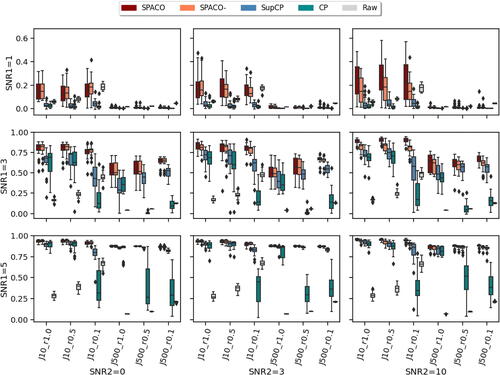
We compare SPACO, SPACO-, plain CP from python package tensorly, and a proxy to SupCP by setting ${\lambda }_{1k}={\lambda }_{2k}={10}^{-2}$ in SPACO as small fixed values (additional small penalties enhance numerical stability when dealing with large q and a high missing rate). Although this is not exactly SupCP, it bears high resemblance. This special case of SPACO is referred to as SupCP, which is included to assess gains from smoothness regularization on the time trajectory. Note that SPACO, SPACO-, and SupCP all employ our proposed initialization, improving stability and performance at high missing rates. An analysis contrasting SupCP with random and proposed initialization is presented in Appendix C.1. In our experiments, we used the true rank for all methods. The accuracy the rank estimation procedure proposed in Section 4.2 is assessed in Appendix C.3. In our experiments, the rank estimation procedure closely approximates the true model rank when the signal is strong, with a tendency to underestimate in cases of weaker signal. This underestimation does not, however, lead to significant increases in reconstruction loss.

Figure 2 shows the achieved correlation between the reconstructed tensors and the underlying signal tensors across various setups and 20 random repetitions. The correlation between two tensors F and $\widehat{F}$ is defined as $〈F_{\text{demean}},{\widehat{F}}_{\mathit{demean}}〉/(⏧F_{\text{demean}}{⏧}_2⏧{\widehat{F}}_{\text{demean}}{⏧}_2)$, where $F_{\text{demean}}$ and ${\widehat{F}}_{\text{demean}}$ are the demeaned version the original and estimated tensors, respectively, and $〈F_{\text{demean}},{\widehat{F}}_{\text{demean}}〉$ is their inner product. Each subplot corresponds to different signal-to-noise ratio combinations (SNR1, SNR2), as indicated by its row and column labels. The y-axis represents the achieved correlation, while the x-axis shows different combinations of J and observation rate. For example, x-axis label $J10\_r0.1$ means the feature dimension is 10, and 10% of entries are observed. The “Raw” method, which correlates the true signal with the empirical observation on non-missing entries, is included to demonstrate signal level in different simulation setups, even though it is not directly comparable to other others in the presence of missing data. A comparison of reconstruction quality on missing entries is provided in Appendix C.2.

Fig. 2 Reconstruction evaluation by the correlation between the estimates and the true signal tensor. In each subplot, the x-axis label indicates different J and observing rate, the y-axis is the achieved correlation, and the box colors represent different methods. The corresponding subplot column/row name represents the signal-to-noise ratio SNR1/SNR2.

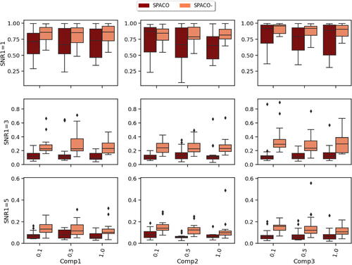
SPACO achieves better reconstruction than SPACO- when subject scores U depend strongly on Z. This is likely due to improved quality in estimating U. To confirm this, we evaluate the estimation quality of U at J = 10 and SNR2$=10$ and measure the estimation quality by R² (regressing the true subject scores on the estimated ones). In Figure 3, we show the achieved $(1-R^2)$ for SPACO and SPACO- (smaller is better), where the x-axis label represents the observing rate and column names represent the component, for example, Comp1$\to U_1$.

Fig. 3 Comparison of SPACO and SPACO- for reconstructing U at J = 10, SNR2$=10$. In each subplot, the x-axis label indicates different component and observing rate, the y-axis is the achieved $(1-R^2)$, and the box colors represent different methods. The corresponding subplot column/row name represents the signal-to-noise ratio SNR1/component.

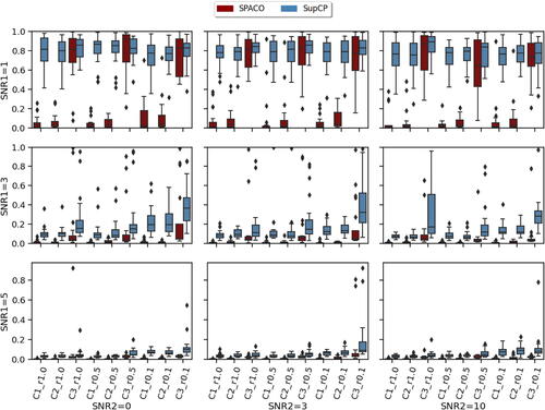
SPACO/SPACO- are both top performers for our smooth tensor decomposition problem and achieve significantly better performance than CP and SupCP when the signal is weak and when the missing rate is high by using the smoothness of the time trajectory. To see this, we compared the estimation quality of the time trajectories using SPACO and SupCP. In Figure 4, we show the achieved $(1-R^2)$ for SPACO and SupCP at J = 10. The x-axis label represents different trajectory and observing rate, for example, $C1\_r1.0$ represents estimation of ${\varphi }_1(t)$ at observing rate r = 1.0. When the signal is weak (SNR1 = 1), SPACO can approximate the constant trajectory component (C1) and begin to estimate other trajectories successfully as the signal increases. SPACO achieves significantly better estimation of the true underlying trajectories than SupCP for various signal-to-noise ratios.

Fig. 4 Comparison of SPACO and SupCP for reconstructing $\Phi$ at J = 10. In each subplot, the x-axis label indicates different component and observing rate, the y-axis is the achieved $(1-R^2)$, and the box colors represent different methods. The corresponding subplot column/row name represents the signal-to-noise ratio SNR1/SNR2.

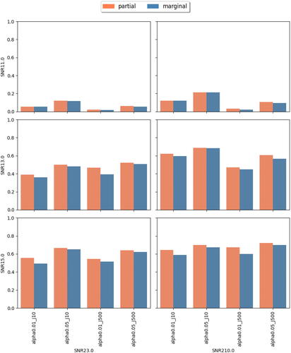
5.2 Variable Importance and Hypothesis Testing

We investigate the approximated p-values based on cross-fit for testing the partial and marginal associations of Z with U under the same simulation set-ups. Since our variables in Z are generated independently, the two null hypotheses coincide. Nevertheless, the two tests have different powers given the same p-value cutoff, as a result of different test statistics adopted. The proposed randomization tests for SPACO achieve reasonable Type I error controls. Using Cross-fit is important for maintaining good Type I error control. In Appendix C.5, we present qq-plots comparing p-values using cross-fitted V and $\Phi$ to the naive construction. The latter exhibits noticeable deviations from the uniform distribution for the later construction when the signal-to-noise ratio is low. Figures 5 and 6 show the achieved Type I error and power with p-value cutoffs at $\alpha =0.01,0.05$ and with an observing rate r = 0.5. The Type I errors are also well controlled for $r\in \{1.0,0.1\}$ (Appendix C.4).

Fig. 5 Achieved Type I errors at observing rate r = 0.5. In each subplot, x-axis label indicates different combination of feature dimension J and targeted level $\alpha \in \{0.01,0.05\}$, while the y-axis represents the achieved Type I errors. Different bar colors represent different tests (partial or marginal). The two dashed horizontal lines correspond to levels 0.01 and 0.05.

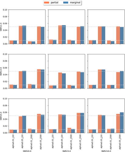
Fig. 6 Achieved power at observing rate r = 0.5. In each subplot, the x-axis label indicates different combinations of feature dimension J and targeted level $\alpha \in \{0.01,0.05\}$, the y-axis indicates the achieved power. Different bar colors represent different tests (partial or marginal).

6 Case Study

SPACO was employed to analyze a longitudinal immunological dataset on COVID-19 obtained from the IMPACT study (Lucas et al. 2020). The original dataset comprised 180 samples collected from 98 COVID-19 infected participants, measuring 135 immunological features. Features with more than 20% missing observations were excluded, and the remaining missing values were imputed using MOFA (Argelaguet et al. 2018) (see Appendix D for more details), resulting a complete matrix of 111 features and 180 samples. This matrix was organized into a sparsely observed tensor of size $(I,T,J)=(98,35,111)$, where T is the number of unique days from symptom onset (DFSO). The average observing rate along the time dimension was 1.84. Additionally, we had access to auxiliary covariates Z containing eight risk factors (COVID_risk1 - COVID_risk5, age, sex, BMI), as well as four symptom measures (ICU, Clinical score, Length of Stay, Coagulopathy). We ran SPACO with X and Z and SPACO- with X only, selecting a model rank of K = 3 based on 5-fold cross-validation. The three estimated components are denoted as C1/C2/C3. Integrating static covariates Z with the longitudinal measurements can sometimes improve the estimation quality of subject scores compared to SPACO-, as demonstrated in our synthetic data examples. While true subject scores are unobtainable in the real dataset, the clinical relevance of the estimated subject scores can still be assessed by comparing them with clinical responses.

SPACO and SPACO- yielded overall highly similar estimations and subject scores, as depicted in Figure 7(A), with the second component exhibiting the largest discrepancy, yet maintaining a correlation above 0.98. Despite this similarity, we observed a noticeable increase in correlations between C2 from SPACO and ICU/Clinical scores/Length of Stay. The permutation p-values from tests on whether the association between these clinical responses are higher with C2 from SPACO than with C2 from SPACO- are 0.006, 0.008, and 0.002 for ICU, Clinical scores and Length of Stay, respectively, as shown in Figure 7(B).

Fig. 7 Comparisons between subject scores estimated from SPACO and SPACO- as well as the static risk factors. Panel A displays the high concordance in the correlations between estimated subject scores from SPACO and SPACO-. Panel B shows the correlations with clinical responses (row label) using subject scores from the most distinct component, C2, estimated with SPACO and SPACO-. The associated permutation p-values, which assess the improvement in correlations with the four clinical responses using SPACO, are shown beneath the row label. Panel C shows the correlation between clinical responses and the two most significant risk factors identified through conditional independence testing, COVIDRISK_3 and BMI.

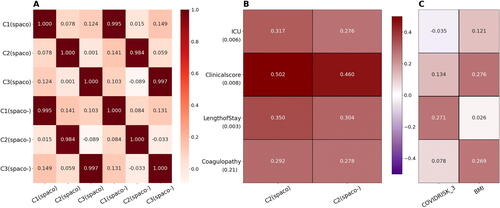
Through the use of the randomization test, we can assess the contribution of each Z_j to C2. Table 1 provides the p-value and adjusted p-value from the conditional independence test, with the number of randomization B = 2000. The top associated risk factor is COVIDRISK_3 (hypertension) with a p-value of 0.001 (adjusted p-value around 0.01). BMI is also weakly associated with C2, with a p-value of 0.07. Both these risk factors displayed much weaker associations with symptom measures when analyzed separately. By including these risk factors in SPACO, the method not only outperforms SPACO-, but also achieves a stronger association with the clinical responses compared to the risk factors themselve (Figure 7(B)–(C)).

Table 1 Results from randomization test for the second component (C2).

	COVIDRISK_1	COVIDRISK_2	COVIDRISK_3	COVIDRISK_4	COVIDRISK_5	Age	sex	BMI
pval	0.958	0.809	0.001	0.268	0.73	0.518	0.762	0.07
padj	0.958	0.924	0.009	0.714	1.00	1.000	1.000	0.28
nz_count	7	24	50	23	5	NaN	47	NaN

NOTE: The column nonzero counts the number of 1 for binary covariate COVIDRISK_1 - COVIDRISK_5 and sex (1 = Male, 0 = Female). The adjusted p-values (padj) are based on BH correction.

7 Discussion

We propose SPACO to model sparse multivariate longitudinal data and auxiliary covariates jointly. The smoothness regularization used in SPACO may lead to a significant improvement in estimation quality, particularly when the missing rate is high. Inclusion of informative auxiliary covariates can also enhance the estimation of subject scores. We applied our proposed pipeline to COVID-19 datasets and demonstrated its effectiveness in identifying components with subject scores that are closely associated with clinical outcomes of interest. Moreover, SPACO can identify static covariates that may contribute to severe symptoms. In the future, we plan to extend SPACO to model multi-omics data, characterized by differing data types, scales, and potentially measurement times. Such an extension will require a tailored model design that carefully integrates the different omics data, rather than a naive approach of blindly pooling them together.

Supplementary Materials

Online Appendices: (Online Appendices.pdf, pdf file) provides additional details of the algorithms, more results from numerical experiments and technical proofs.

Experiment Code: (SPACOexperiments.zip, zip file) It contains code for reproducing results in synthetic and real data experiments, and organized read dataset. A README.md document has been included to for detailed instructions on how to reproduce results represented in this article. Contents in this zip file can also be found at https://github.com/LeyingGuan/SPACOexperments.

Python package for SPACO: (SPACO.zip, zip file) It contains the Python implementation of the SPACO package. Readers can also find and install SPACO from GitHub at https://github.com/LeyingGuan/SPACO.

Acknowledgments

We express our gratitude to the editor, associate editor, and two reviewers for their insightful feedback, which has substantially enhanced the article.

Disclosure Statement

The author reports there are no competing interests to declare.

Additional information

Funding

L.G. was supported in part by the NSF award DMS-2310836.

References

- Acar, E., and Yener, B. (2008), “Unsupervised Multiway Data Analysis: A Literature Survey,” IEEE Transactions on Knowledge and Data Engineering, 21, 6–20. DOI: 10.1109/TKDE.2008.112.
- Anderlucci, L., and Viroli, C. (2015), “Covariance Pattern Mixture Models for the Analysis of Multivariate Heterogeneous Longitudinal Data,” The Annals of Applied Statistics, 9, 777–800. DOI: 10.1214/15-AOAS816.
- Argelaguet, R., Velten, B., Arnol, D., Dietrich, S., Zenz, T., Marioni, J. C., Buettner, F., Huber, W., and Stegle, O. (2018), “Multi-Omics Factor Analysis–A Framework for Unsupervised Integration of Multi-Omics Data Sets,” Molecular Systems Biology, 14, e8124. DOI: 10.15252/msb.20178124.
- Bai, J., and Wang, P. (2015), “Identification and Bayesian Estimation of Dynamic Factor Models,” Journal of Business & Economic Statistics, 33, 221–240. DOI: 10.1080/07350015.2014.941467.
- Bai, J., and Wang, P. (2016), “Econometric Analysis of Large Factor Models,” Annual Review of Economics, 8, 53–80. DOI: 10.1146/annurev-economics-080315-015356.
- Berrett, T. B., Wang, Y., Barber, R. F., and Samworth, R. J. (2020), “The Conditional Permutation Test for Independence While Controlling for Confounders,” Journal of the Royal Statistical Society, Series B, 82, 175–197. DOI: 10.1111/rssb.12340.
- Besse, P., and Ramsay, J. O. (1986), “Principal Components Analysis of Sampled Functions,” Psychometrika, 51, 285–311. DOI: 10.1007/BF02293986.
- Bro, R., and Andersson, C. A. (1998), “Improving the Speed of Multiway Algorithms: Part II: Compression,” Chemometrics and Intelligent Laboratory Systems, 42, 105–113. DOI: 10.1016/S0169-7439(98)00011-2.
- Candes, E., Fan, Y., Janson, L., and Lv, J. (2018), “Panning for Gold: ‘model-x’ Knockoffs for High Dimensional Controlled Variable Selection,” Journal of the Royal Statistical Society, Series B, 80, 551–577. DOI: 10.1111/rssb.12265.
- Carroll, J. D., Pruzansky, S., and Kruskal, J. B. (1980), “Candelinc: A General Approach to Multidimensional Analysis of Many-Way Arrays with Linear Constraints on Parameters,” Psychometrika, 45, 3–24. DOI: 10.1007/BF02293596.
- Chang, W.-C. (1983), “On Using Principal Components before Separating a Mixture of Two Multivariate Normal Distributions,” Journal of the Royal Statistical Society, Series C, 32, 267–275. DOI: 10.2307/2347949.
- Chen, E. Y., Tsay, R. S., and Chen, R. (2020), “Constrained Factor Models for High-Dimensional Matrix-Variate Time Series,” Journal of the American Statistical Association, 115, 775–793. DOI: 10.1080/01621459.2019.1584899.
- De Lathauwer, L., De Moor, B., and Vandewalle, J. (2000), “A Multilinear Singular Value Decomposition,” SIAM Journal on Matrix Analysis and Applications, 21, 1253–1278. DOI: 10.1137/S0895479896305696.
- Efron, B., Tibshirani, R., Storey, J. D., and Tusher, V. (2001), “Empirical Bayes Analysis of a Microarray Experiment,” Journal of the American Statistical Association, 96, 1151–1160. DOI: 10.1198/016214501753382129.
- Ernst, M. D. (2004), “Permutation Methods: A Basis for Exact Inference,” Statistical Science, 19, 676–685. DOI: 10.1214/088342304000000396.
- Fan, J., Fan, Y., and Lv, J. (2008), “High Dimensional Covariance Matrix Estimation Using a Factor Model,” Journal of Econometrics, 147, 186–197. DOI: 10.1016/j.jeconom.2008.09.017.
- Fan, J., Liao, Y., and Mincheva, M. (2011), “High Dimensional Covariance Matrix Estimation in Approximate Factor Models,” Annals of Statistics, 39, 3320–3356. DOI: 10.1214/11-AOS944.
- Fisher, R. A. (1936), “Design of Experiments,” British Medical Journal, 1, 554. DOI: 10.1136/bmj.1.3923.554-a.
- Harshman, R. A., and Lundy, M. E. (1994), “Parafac: Parallel Factor Analysis,” Computational Statistics & Data Analysis, 18, 39–72. DOI: 10.1016/0167-9473(94)90132-5.
- Hinrich, J. L., and Mørup, M. (2019), “Probabilistic Tensor Train Decomposition,” in 2019 27th European Signal Processing Conference (EUSIPCO), pp. 1–5, IEEE. DOI: 10.23919/EUSIPCO.2019.8903177.
- Huang, J. Z., Shen, H., and Buja, A. (2008),“Functional Principal Components Analysis via Penalized Rank One Approximation,” Electronic Journal of Statistics, 2, 678–695. DOI: 10.1214/08-EJS218.
- Imaizumi, M., and Hayashi, K. (2017), “Tensor Decomposition with Smoothness,” in International Conference on Machine Learning, pp. 1597–1606, PMLR.
- Kolda, T. G., and Bader, B. W. (2009), “Tensor Decompositions and Applications,” SIAM Review, 51, 455–500. DOI: 10.1137/07070111X.
- Lam, C., Yao, Q., and Bathia, N. (2011), “Estimation of Latent Factors for High-Dimensional Time Series,” Biometrika, 98, 901–918. DOI: 10.1093/biomet/asr048.
- Li, G., Shen, H., and Huang, J. Z. (2016), “Supervised Sparse and Functional Principal Component Analysis,” Journal of Computational and Graphical Statistics, 25, 859–878. DOI: 10.1080/10618600.2015.1064434.
- Lock, E. F., and Li, G. (2018), “Supervised Multiway Factorization,” Electronic Journal of Statistics, 12, 1150–1180. DOI: 10.1214/18-EJS1421.
- Lucas, C., Wong, P., Klein, J., Castro, T. B., Silva, J., Sundaram, M., Ellingson, M. K., Mao, T., Oh, J. E., Israelow, B., et al. (2020), “Longitudinal Analyses Reveal Immunological Misfiring in Severe Covid-19,” Nature, 584, 463–469. DOI: 10.1038/s41586-020-2588-y.
- Mnih, A., and Salakhutdinov, R. R. (2007), “Probabilistic Matrix Factorization,” in Advances in Neural Information Processing Systems (Vol. 20), pp. 1257–1264.
- Onghena, P. (2017), “Randomization Tests or Permutation Tests? A Historical and Terminological Clarification,” in Randomization, Masking, and Allocation Concealment, pp. 209–228, New York: Chapman and Hall/CRC.
- Phan, A.-H., Tichavskỳ, P., and Cichocki, A. (2013), “Candecomp/parafac Decomposition of High-Order Tensors through Tensor Reshaping,” IEEE Transactions on Signal Processing, 61, 4847–4860. DOI: 10.1109/TSP.2013.2269046.
- Pitman, E. J. G. (1937), “Significance Tests Which May be Applied to Samples from any Populations. II. The Correlation Coefficient Test,” Supplement to the Journal of the Royal Statistical Society, 4, 225–232. DOI: 10.2307/2983647.
- Rendeiro, A. F., Casano, J., Vorkas, C. K., Singh, H., Morales, A., DeSimone, R. A., Ellsworth, G. B., Soave, R., Kapadia, S. N., Saito, K., et al. (2021), “Profiling of Immune Dysfunction in Covid-19 Patients Allows Early Prediction of Disease Progression,” Life Science Alliance, 4, e202000955. DOI: 10.26508/lsa.202000955.
- Sidiropoulos, N. D., De Lathauwer, L., Fu, X., Huang, K., Papalexakis, E. E., and Faloutsos, C. (2017), “Tensor Decomposition for Signal Processing and Machine Learning,” IEEE Transactions on Signal Processing, 65, 3551–3582. DOI: 10.1109/TSP.2017.2690524.
- Sorkine, O., Cohen-Or, D., Lipman, Y., Alexa, M., Rössl, C., and Seidel, H.-P. (2004), “Laplacian Surface Editing,” in Proceedings of the 2004 Eurographics/ACM SIGGRAPH symposium on Geometry processing, pp. 175–184.
- Tibshirani, R. (2011), “Regression Shrinkage and Selection via the Lasso: A Retrospective,” Journal of the Royal Statistical Society, Series B, 73, 273–282. DOI: 10.1111/j.1467-9868.2011.00771.x.
- Tipping, M. E., and Bishop, C. M. (1999), “Probabilistic Principal Component Analysis,” Journal of the Royal Statistical Society, Series B, 61, 611–622. DOI: 10.1111/1467-9868.00196.
- Vichi, M., Rocci, R., and Kiers, H. A. (2007), “Simultaneous Component and Clustering Models for Three-Way Data: Within and between Approaches,” Journal of Classification, 24, 71–98. DOI: 10.1007/s00357-007-0006-x.
- Viroli, C. (2011), “Finite Mixtures of Matrix Normal Distributions for Classifying Three-Way Data,” Statistics and Computing, 21, 511–522. DOI: 10.1007/s11222-010-9188-x.
- Wang, D., Liu, X., and Chen, R. (2019), “Factor Models for Matrix-Valued High-Dimensional Time Series,” Journal of Econometrics, 208, 231–248. DOI: 10.1016/j.jeconom.2018.09.013.
- Wang, D., Zheng, Y., Lian, H., and Li, G. (2021), “High-Dimensional Vector Autoregressive Time Series Modeling via Tensor Decomposition,” Journal of the American Statistical Association, 117, 1338–1356. DOI: 10.1080/01621459.2020.1855183.
- Yao, F., Müller, H.-G., and Wang, J.-L. (2005), “Functional Data Analysis for Sparse Longitudinal Data,” Journal of the American Statistical Association, 100, 577–590. DOI: 10.1198/016214504000001745.
- Yokota, T., Zhao, Q., and Cichocki, A. (2016), “Smooth Parafac Decomposition for Tensor Completion,” IEEE Transactions on Signal Processing, 64, 5423–5436. DOI: 10.1109/TSP.2016.2586759.