Vecchia Likelihood Approximation for Accurate and Fast Inference with Intractable Spatial Max-Stable Models

Abstract

Max-stable processes are the most popular models for high-impact spatial extreme events, as they arise as the only possible limits of spatially-indexed block maxima. However, likelihood inference for such models suffers severely from the curse of dimensionality, since the likelihood function involves a combinatorially exploding number of terms. In this article, we propose using the Vecchia approximation, which conveniently decomposes the full joint density into a linear number of low-dimensional conditional density terms based on well-chosen conditioning sets designed to improve and accelerate inference in high dimensions. Theoretical asymptotic relative efficiencies in the Gaussian setting and simulation experiments in the max-stable setting show significant efficiency gains and computational savings using the Vecchia likelihood approximation method compared to traditional composite likelihoods. Our application to extreme sea surface temperature data at more than a thousand sites across the entire Red Sea further demonstrates the superiority of the Vecchia likelihood approximation for fitting complex models with intractable likelihoods, delivering significantly better results than traditional composite likelihoods, and accurately capturing the extremal dependence structure at lower computational cost. Supplementary materials for this article are available online.

Keywords:

• Asymptotic relative efficiency
• Composite likelihood
• Gaussian process
• Max-stable process
• Vecchia approximation

1 Introduction

Max-stable models have been used extensively for describing the dependence structure in multivariate and spatial extremes (Padoan, Ribatet, and Sisson 2010; Segers 2012; Davis, Küppelberg, and Steinkohl 2013; de Carvalho and Davison 2014; Huser and Davison 2014; Huser and Genton 2016). They are natural models to use since they are characterized by the max-stability property, arising in limiting joint distributions for block maxima with block size tending to infinity; see the reviews by Davison, Padoan, and Ribatet (2012), Davison and Huser (2015), and Davison, Huser, and Thibaud (2019).

However, likelihood-based inference for high-dimensional max-stable distributions is computationally prohibitive (Padoan, Ribatet, and Sisson 2010; Castruccio, Huser, and Genton 2016). Although the likelihood function has a known general expression, it involves a combinatorial explosion of terms, which makes it impossible to evaluate it exactly, even in relatively small dimensions. In classical geostatistics, Gaussian graphical models, which are represented in terms of a conditional independence graph, play a key role for modeling big spatial data as they lead to Gaussian Markov random fields (Rue and Held 2005), which have a sparse precision (i.e., inverse covariance) matrix and are directly linked to certain classes of continuous-spaceGaussian stochastic partial equation models (Lindgren, Rue, and Lindström 2011). Thanks to the Hammersley–Clifford Theorem, the joint density of graphical models can be decomposed into lower-dimensional densities according to the underlying graph, thus, making computations much faster. In the extremes context, recent work has shown how to build graphical models for multivariate extremes based on high threshold exceedances modeled through the multivariate Pareto distribution (Engelke and Hitz 2020; Engelke and Ivanovs 2021). However, interestingly, it is possible to show that conditional independence in max-stable models with a continuous joint density only yields full independence (Papastathopoulos and Strokorb 2016). This implies that nontrivial Markov max-stable models do not exist, and thus, that likelihood-based inference for max-stable processes is not just a challenging task; it is, by nature of the problem, intrinsically difficult. In other words, this computational bottleneck is “built-in”, and cannot be easily bypassed. Nevertheless, viable inference solutions need to be found.

For some very specific classes of max-stable models, fast methods can still be designed: the likelihood function for the logistic and nested logistic multivariate models can be efficiently computed using a recursive formula (see Shi 1995; Vettori et al. 2020), while the hierarchical construction of the Reich–Shaby max-stable spatial process can be exploited to perform Bayesian inference in high dimensions (Reich and Shaby 2012; Stephenson et al. 2015; Vettori, Huser, and Genton 2019; Bopp, Shaby, and Huser 2021). Apart from these restrictive cases, full likelihood inference for max-stable models is extremely intensive, and this has prevented the use of more flexible max-stable classes, such as the Brown–Resnick (Kabluchko, Schlather, and de Haan 2009) or extremal-t (Opitz 2013) processes, in high-dimensional settings. Recent attempts have succeeded in fitting the Brown–Resnick process in dimension $D\approx 20$ based on the full likelihood, either using an astute stochastic expectation–maximization algorithm (Huser et al. 2019) or a Markov chain Monte Carlo algorithm in the Bayesian framework (Thibaud et al. 2016; Dombry, Engelke, and Oesting 2017). Nevertheless, these approaches remain difficult to apply in higher dimensions. Alternatively, Stephenson and Tawn (2005) have proposed a full likelihood approach based on the occurrence times of maxima, but Wadsworth (2015) and Huser, Davison, and Genton (2016) have found that this is often severely biased in low dependence situations. More recently, Lenzi et al. (2023) and Sainsbury-Dale, Zammit-Mangion, and Huser (2023) proposed using neural networks for parameter estimation in intractable models, including max-stable processes. They showed that considerable time savings can be obtained, though training neural networks for parameter estimation requires model-specific tuning; this may become especially tricky as the number of parameters increases. Furthermore, as is often the case with machine learning approaches, statistical guarantees are usually more difficult to get, especially as far as asymptotics and uncertainty quantification are concerned.

To make inference for max-stable processes, Padoan, Ribatet, and Sisson (2010) initially suggested using a pairwise (composite) likelihood, which is built by combining bivariate densities that are possibly weighted to improve statistical and computational efficiency. The benefits of this approach are that (i) it is simple to implement; (ii) it yields dramatic reductions in computational burden with respect to a full likelihood-based approach; and (iii) large-sample properties of composite likelihood estimators are well understood. The main drawback is that it leads to some considerable loss in efficiency due to using only the information contained in pairs of variables. Similarly, a pairwise M-estimator was proposed by Einmahl et al. (2016), with optimal, data-driven weights to improve statistical efficiency. In the same spirit, Padoan, Ribatet, and Sisson (2010) suggested selecting only close-by pairs of sites, that is, using binary weights set according to the distance between sites, and choosing the cutoff distance in a way that minimizes the trace of the estimator’s asymptotic variance. Although this improves the estimator, it is still quite far from optimal, especially in high-dimensional settings. Alternatively, Genton, Ma, and Sang (2011), Huser and Davison (2013), Sang and Genton (2014), Castruccio, Huser, and Genton (2016), and Beranger, Stephenson, and Sisson (2021) have explored triplewise and higher-order composite likelihoods, and have shown that significant efficiency gains can be obtained by using truncated composite likelihoods, that is, by choosing the marginal likelihood components from subsets of sites that are contained within a disk of fixed radius. However, this approach is still not very attractive in large dimensions D, because it is costly to enumerate all the $(\begin{array}{c}D\\ d\end{array})$ marginal likelihood components that are built from $2\le d\le D$ sites, and to identify and evaluate those that are contained within a disk of radius $\delta >0$. Moreover, unless the truncation distance δ is very small, the number of such selected components may still be too large to be practical in high dimensions D. To further reduce the computational time when fitting intractable models such as max-stable processes, Whitaker, Beranger, and Sisson (2020) proposed using pairwise likelihoods for histogram-valued variables, obtained by discretizing the sample space into rectangles and summarizing the data as counts in each discretized bin. However, while this “symbolic data analysis” approach offers computational savings, it further deteriorates the estimator’s statistical efficiency and it does not scale well with composite likelihoods of higher order.

In this article, we propose making inference for max-stable processes by leveraging the Vecchia approximation (Vecchia 1988). Essentially, the joint density of the data is approximated by a product of well-chosen lower-dimensional conditional densities. Therefore, as explained in Section 2, it can be viewed as a particular type of (weighted) composite likelihood. However, unlike the classical pairwise or higher-order composite likelihood approaches considered previously in the extreme-value literature, the Vecchia approximation provides by construction a valid likelihood function, in the sense that it corresponds to the joint density of a well-defined data generating process that approximates the true process under study. Moreover, the number of conditional densities to compute is proportional to the dimension D. For these reasons, the Vecchia approximation has been found in the Gaussian-based geostatistical setting not only to provide fast inference for big datasets, but also to generally retain high efficiency compared to full likelihood approaches and to outperform block composite likelihoods (Stein, Chi, and Welty 2004; Katzfuss et al. 2020; Katzfuss and Guinness 2021). The Vecchia approximation has not been explored for intractable non-Gaussian extremes models yet, though Nascimento and Shaby (2022) is a recent related contribution, where the Vecchia approximation is exploited to provide fast and accurate approximations of multivariate Gaussian distribution functions, which are then used for censored likelihood inference in Gaussian scale mixture models for spatial extremes.

The Vecchia approximation relies on the choice of three elements: (i) a permutation defining an ordering of spatial sites; (ii) the number of conditioning sites; and (iii) the conditioning sets themselves. While this flexibility might be seen as a limitation, Guinness (2018) instead argues that it can be exploited to improve the approximation. Based on simulation results, Guinness (2018) suggested using a maximum–minimum distance ordering, which provides some improvements over coordinate-based orderings. In order to study the exact effect that these three choices have on the Vecchia approximation, and to do a formal comparison with classical composite likelihood approaches, we study in the supplementary materials the theoretical asymptotic relative efficiency of these different estimators in the Gaussian setting for various correlation models. Our new results complement the theoretical results of Stein, Chi, and Welty (2004) and the numerical results of Guinness (2018), Katzfuss et al. (2020), and Katzfuss and Guinness (2021). In Section 3, we conduct an extensive simulation study to extend these results to the popular Brown–Resnick max-stable model and detail further results for the multivariate logistic max-stable model in the supplementary materials. Our results for the Gaussian and max-stable cases provide evidence that the Vecchia approximation yields competitively efficient estimators and attractive computational savings, while scaling well with the dimension. We use our results to provide guidance on the choice of the ordering and conditioning sets in the max-stable setting. In Section 4, we then exploit the Vecchia approximation to study sea surface temperature extremes for the whole Red Sea at more than a thousand sites. We demonstrate the advantages of using the Vecchia approximation method compared to traditional composite likelihoods. Section 5 concludes with some discussion and a perspective on future research.

2 Inference based on Composite Likelihoods and the Vecchia Approximation

2.1 Composite Likelihoods and Choice of Weights

Consider a D-dimensional random vector $\mathit{Z}\in {\mathbb{R}}^D$ with density $f(\mathit{z};\mathit{\psi }),\mathit{z}\in \mathcal{Z}\subset {\mathbb{R}}^D$, parameterized in terms of a m-dimensional vector $\mathit{\psi }={({\psi }_1,\dots ,{\psi }_m)}^{\top }\in \Psi \subseteq {\mathbb{R}}^m$. Marginal densities of all subvectors are also denoted by f, for simplicity. Suppose that the true parameter vector is ${\mathit{\psi }}_0\in \text{Int}(\Psi )$. Then, a composite log-likelihood for n independent realizations ${\mathit{z}}_1,\dots ,{\mathit{z}}_n$ of the random vector Z may be defined as ${\mathcal{l}}_C(\mathit{\psi })={\sum }_{i=1}^n{\mathcal{l}}_C(\mathit{\psi };{\mathit{z}}_i)$, where (1) $${\mathcal{l}}_C(\mathit{\psi };\mathit{z})=\sum _{S\in C_D}{w}_S\hspace{0.17em}\log \hspace{0.17em}f({\mathit{z}}_S;\mathit{\psi })=\sum _{d=1}^D\sum _{S\in C_{D;d}}{w}_S\hspace{0.17em}\log \hspace{0.17em}f({\mathit{z}}_S;\mathit{\psi }),$$(1) where $C_D={\cup }_{d=1}^D{C}_{D;d}$ is the collection of all non-empty subsets of $\{1,\dots ,D\},C_{D;d}$ is the collection of all d-dimensional subsets of $\{1,\dots ,D\}$, and $w_S\in \mathbb{R}$ is a weight attributed to subset S. We write ${\mathit{z}}_S$ to denote the subvectors obtained by restricting z to the components indexed by the subset S. The maximum composite likelihood estimator (MCLE) is defined as ${\widehat{\mathit{\psi }}}_C=\arg {\max }_{\mathit{\psi }\in \Psi }{\mathcal{l}}_C(\mathit{\psi })$. Provided all likelihood terms involved in (1) satisfy the Bartlett identities, the gradient of (1) with respect to $\mathit{\psi }$ is an unbiased estimating equation, and thus the classical asymptotic theory can be applied. If $\mathit{\psi }$ is identifiable from the likelihood terms with nonzero weight in (1), then under mild regularity conditions, ${\widehat{\mathit{\psi }}}_C$ is consistent and asymptotically normal as $n\to \infty$ and the variance-covariance matrix of ${\widehat{\mathit{\psi }}}_C$ can be approximated by $\mathit{V}=n^{-1}{\mathit{J}}^{-1}({\mathit{\psi }}_0)\mathit{K}({\mathit{\psi }}_0){\mathit{J}}^{-1}({\mathit{\psi }}_0)$ for large n, where $\mathit{J}(\mathit{\psi })=\mathrm{E}\{-\frac{{\partial }^2}{\partial \mathit{\psi }\partial \mathit{\psi }}{\mathcal{l}}_C(\mathit{\psi };\mathit{Z})\}$ is the sensitivity matrix and $\mathit{K}(\mathit{\psi })=\text{var}\{\frac{\partial }{\partial \mathit{\psi }}{\mathcal{l}}_C(\mathit{\psi };\mathit{Z})\}$ is the variability matrix; see, for example, Varin, Reid, and Firth (2011). The choice of weights w_S in (1) turns out to be crucial for the estimator’s efficiency. Although weights are often assumed to be nonnegative (Varin, Reid, and Firth 2011), this is non-necessarily restrictive and Pace, Salvan and Sartori (2019) show that optimal weights may in some cases be negative; see also Fraser and Reid (2020). As the sum in (1) involves $2^D-1$ terms, some weights w_S are often set to zero for computations.

Composite marginal log-likelihoods of order $d=1,2,\dots ,D$ are defined by setting w_S = 0 in (1) for all subsets $S\subset \{1,\dots ,D\}$ with cardinality $\left|S\right|\ne d$. The corresponding composite log-likelihood may be written as ${\mathcal{l}}_{C;d}(\mathit{\psi })={\sum }_{i=1}^n{\mathcal{l}}_{C;d}(\mathit{\psi };{\mathit{z}}_i)$ with (2) $${\mathcal{l}}_{C;d}(\mathit{\psi };\mathit{z})=\sum _{S\in C_{D;d}}{w}_S\hspace{0.17em}\log \hspace{0.17em}f({\mathit{z}}_S;\mathit{\psi }).$$(2)

We write ${\widehat{\mathit{\psi }}}_{C;d}$ to denote the mode (i.e., $\arg \max$) of ${\mathcal{l}}_{C;d}(\mathit{\psi })$. The definition (2) includes pairwise (d = 2) or triplewise (d = 3) likelihoods that were advocated by Padoan, Ribatet, and Sisson (2010), Genton, Ma, and Sang (2011), and Huser and Davison (2013) as a method of inference for max-stable processes, for which the full likelihood is intractable in large dimensions D. Castruccio, Huser, and Genton (2016) also investigated higher-order composite likelihoods of the form (2) and reported efficiency gains for increasing d. The choice of weights w_S in pairwise likelihoods is not trivial. In the context of max-stable processes, Padoan, Ribatet, and Sisson (2010) suggest using binary weights $w_S=\mathbb{I}(\Vert {\mathit{h}}_S\Vert \le \delta )$, for some cutoff distance $\delta >0$, where $\Vert {\mathit{h}}_S\Vert$ denotes the distance between the pair of sites indexed by the set S and $\mathbb{I}(·)$ is the indicator function, while they choose δ by minimizing an estimate of the asymptotic variance V. This approach leads to efficiency gains as opposed to using equal weights, that is, w_S = 1 for all S, but it may not be optimal. Huser (2013), Chapter 3, studies the efficiency of pairwise likelihood estimators for Gaussian and max-stable time series models, and provide some further guidance on the choice of weights. For higher-order composite likelihoods with d > 2, it is even less clear how to select the weights w_S optimally, and by analogy to the pairwise likelihood setting, Sang and Genton (2014) and Castruccio, Huser, and Genton (2016) have suggested adopting a truncated composite likelihood approach, which uses weights of the type $w_S=\mathbb{I}({\max }_{\{i,j\}\subset S}\Vert {\mathit{h}}_{\{i,j\}}\Vert \le \delta )$ for some cutoff distance $\delta >0$, thus, discarding d-dimensional subsets with pairs of sites that are distant from each other.

2.2 Vecchia Approximation

The Vecchia approximation (Vecchia 1988) relies on the simple fact that the joint density can be written as the product of conditional densities; see also Stein, Chi, and Welty (2004). Consider the vector $\mathit{z}={(z_1,\dots ,z_D)}^{\top }\in {\mathbb{R}}^D$ and a permutation $p:\{1,\dots ,D\}\mapsto \{1,\dots ,D\}$, which defines a re-ordering of the variables z_j, $j=1,\dots ,D$. We define the “history” of the jth variable based on the permutation p as the subvector ${\mathit{z}}_{H(j;p)}$, where $H(j;p)=\{l\in \{1,\dots ,D\}:p(l)<p(j)\}$ denotes the index set of “past” variables. Then, for any choice of permutation p, the joint density may be expressed as (3) $$f(\mathit{z};\mathit{\psi })=f(z_{p(1)};\mathit{\psi })\prod _{j=2}^{D}f(z_{p(j)}|{\mathit{z}}_{H(j;p)};\mathit{\psi }).$$(3)

The Vecchia approximation consists in replacing the history ${\mathit{z}}_{H(j;p)}$ in (3) with a subvector ${\mathit{z}}_{S(j;p)}$, with $S(j;p)\subseteq H(j;p)$, that is, (4) $$f_V(\mathit{z};\mathit{\psi }):=f(z_{p(1)};\mathit{\psi })\prod _{j=2}^{D}f(z_{p(j)}|{\mathit{z}}_{S(j;p)};\mathit{\psi })\approx f(\mathit{z};\mathit{\psi }).$$(4)

A counterpart of (4) based on blocks of variables is also considered in Stein, Chi, and Welty (2004). While the permutation p is irrelevant for the full density in (3), it affects the approximation (4). As opposed to time series data, there is no natural ordering of variables in the spatial setting, and although Stein, Chi, and Welty (2004) argues that it has a negligible impact on the quality of the Vecchia approximation, Guinness (2018) instead suggests that certain orderings have a better performance than simple coordinate-based orderings. As Stein, Chi, and Welty (2004) and Katzfuss and Guinness (2021) show, the Vecchia approximation crucially depends on the size of the conditioning sets $S(j;p)$, which implies that there is a tradeoff between approximation accuracy and computational efficiency. Usually, a compromise is adopted between singletons of cardinality $|S(j;p)|=1$ (with low computational burden but poor approximation) and maximal sets of cardinality $|S(j;p)|=p(j)-1$ as with the full likelihood (with perfect approximation but heavy computational burden). Here, we choose to restrict the cardinality to $|S(j;p)|=\min (p(j),d)-1$, for some lower dimension $2\le d\le D$. Typically, the “cutoff dimension” d will be quite small, which dramatically reduces the computational burden. Finally, the Vecchia approximation (4) also depends on the specific choice of variables to include in the sub-history $S(j;p)$. We here follow the original paper of Vecchia (1988) who in the spatial context suggest including the $\min (p(j),d)-1$ nearest neighbors of the jth site among those that belong to its history, $H(j;p)$. Thereafter, we write $S(j;p)\equiv S_{d-1}(j;p)$ to stress that the dimensionality of the conditioning sets is at most d–1.

The log-likelihood based on the Vecchia approximation (4) may be written in composite likelihood form as in (1). Precisely, it may be expressed as (5) $$\begin{array}{c}{\mathcal{l}}_{V;d}(\mathit{\psi };\mathit{z})=\hspace{0.17em}\log \hspace{0.17em}{f}_{V;d}(\mathit{z};\mathit{\psi })\\ =\hspace{0.17em}\log \hspace{0.17em}f(z_{p(1)};\mathit{\psi })+\sum _{j=2}^D\hspace{0.17em}\log \hspace{0.17em}f(z_{p(j)},{\mathit{z}}_{S_{d-1}(j;p)};\mathit{\psi })\\ -\sum _{j=2}^D\hspace{0.17em}\log \hspace{0.17em}f({\mathit{z}}_{S_{d-1}(j;p)};\mathit{\psi }),\end{array}$$(5) where D composite likelihood weights w_S in (1) are set to 1, D–1 weights are set to–1, and the rest are set to zero. There are thus only $2D-1$ likelihood terms to evaluate in (5), as opposed to ${\sum }_{d=1}^D(\begin{array}{c}D\\ d\end{array})=2^D-1$ terms in (1) and $(\begin{array}{c}D\\ d\end{array})$ terms in (2) (when $w_S\ne 0$ for all S). We stress that the number of likelihood terms to compute drives the computational complexity of each estimator, and thus, for fixed d, the Vecchia likelihood estimator will typically have lower computational complexity than its composite likelihood counterpart as a function of D. The dimension of densities involved in (5) is at most d, and thus, is in some sense comparable to (2). We write ${\widehat{\mathit{\psi }}}_{V;d}$ to denote the mode (i.e., $\arg \max$) of ${\mathcal{l}}_{V;d}(\mathit{\psi })={\sum }_{i=1}^n{\mathcal{l}}_{V;d}(\mathit{\psi };{\mathit{z}}_i)$, with ${\mathcal{l}}_{V;d}(\mathit{\psi };\mathit{z})$ defined in (5), and because of the analogy between (5) and (1), the same asymptotic theory applies, although ${\widehat{\mathit{\psi }}}_{V;d}$ usually provides gains in efficiency as compared to ${\widehat{\mathit{\psi }}}_{C;d}$; see the results in Section 3 and the supplementary materials. We also note that both traditional composite and Vecchia likelihood approaches have the benefit of being “robust” against misspecification of the likelihood components that are not involved. Therefore, for the same value of d, both approaches will have comparable robustness properties and will be insensitive to wrong assumptions about higher-order dependencies (i.e., of order $\ge d+1$).

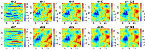
Notice that because the Vecchia approximation relies on a nested sequence of conditional events, the expression (4) is by construction a valid likelihood function that corresponds to a specific data generating process (Katzfuss and Guinness 2021), as opposed to pairwise likelihoods or more general composite likelihoods as in (1). As such, it avoids using “redundant” information, which is key to improving the estimator’s efficiency. As illustrated in Figure 1, the Vecchia likelihood approximation actually yields an approximation of the process itself. The larger the cutoff dimension d, the better the approximation, as expected. For small cutoff dimensions d, the approximation fails at accurately representing the full joint distribution, although it captures the low-dimensional interactions reasonably well. The choice of a coordinate-based ordering for the Vecchia approximation is apparent for d = 2, but the approximation improves dramatically as d increases. In fact, since the Vecchia likelihood approximation is a valid likelihood function (thus, a density), it is possible to measure the quality of the approximation by considering the Kullback–Leibler (KL) divergence of $f_{V;d}(\mathit{z})$ with respect to the true likelihood $f(\mathit{z})$ (with dependence on $\mathit{\psi }$ suppressed for readability), that is, $\text{KL}(f\Vert f_{V;d})=\int f(\mathit{z})\hspace{0.17em}\log \hspace{0.17em}\{f(\mathit{z})/f_{V;d}(\mathit{z})\}\mathrm{d}\mathit{z}$; see, for example, Schäfer, Katzfuss, and Owhadi (2021) for some approximation results in the Gaussian case. When subsets $S_{d-1}(j;p)$ are chosen as the nearest neighbors from the jth site, we can show that, in the general (potentially non-Gaussian) case, $\text{KL}(f\Vert f_{V;d})$ is always a nonincreasing function of d, that is, the Vecchia approximate likelihood gets “closer and closer” to the true likelihood, as expected. This result is formalized in Proposition 1 of the supplementary materials (see also Proposition 2 in Katzfuss et al. (2020) for the Gaussian case). Notice that this does usually not hold for general (renormalized) composite likelihoods. The illustration in Figure 1 also implies that the approximation improves as d increases. This suggests that a similar improvement is to be expected in terms of the relative efficiency of the corresponding Vecchia likelihood estimator, ${\widehat{\mathit{\psi }}}_{V;d}$. Although the Vecchia log-likelihood in (5) is appealing and has good efficiency, there is no reason why the corresponding weights $w_S\in \{-1,0,1\}$ should necessarily be optimal. In the supplementary materials, we also explore a modified Vecchia likelihood obtained by changing the weights attributed to the conditioning sets.

Fig. 1 Realizations from Gaussian processes on ${\{1,\dots ,32\}}^2$ with zero mean, unit variance, and correlation function $\text{corr}\{Z(\mathit{s}),Z(\mathit{s}+\mathit{h})\}=\hspace{0.17em}\exp \hspace{0.17em}(-\Vert \mathit{h}\Vert /5)$ (top right) and $\text{corr}\{Z(\mathit{s}),Z(\mathit{s}+\mathit{h})\}=\hspace{0.17em}\exp \hspace{0.17em}\{-{(\Vert \mathit{h}\Vert /5)}^{1.5}\}$ (bottom right), and their corresponding Vecchia approximations for $d=2,3,5,13$ (from left to right), using a coordinate-based ordering.

3 Simulation Study in the Max-Stable Case

3.1 Max-Stable Models

As already noted, max-stable processes are the only possible limits of suitably renormalized pointwise maxima of independent and identically distributed random fields. More specifically, let $Y_1(\mathit{s}),Y_2(\mathit{s}),\dots$ denote independent copies of the random field $Y(\mathit{s})$, $\mathit{s}\in {\mathbb{R}}^2$, and let $\{M_n(\mathit{s})\equiv \max \{Y_1(\mathit{s}),\dots ,Y_n(\mathit{s})\},\mathit{s}\in {\mathbb{R}}^2\}$ be the process of pointwise maxima. Furthermore, assume that $Y(\mathit{s})$ satisfies the max-domain of attraction condition, that is, there exist sequences $a_n(\mathit{s})>0$ and $b_n(\mathit{s})$ such that $a_n^{-1}(\mathit{s})\{M_n(\mathit{s})-b_n(\mathit{s})\}\stackrel{D}{\to }Z(\mathit{s})$, where the convergence holds in the sense of finite-dimensional distributions and the limit process $Z(\mathit{s})$ has nondegenerate margins. Then, $Z(\mathit{s})$ is a max-stable process, with generalized extreme-value (GEV) marginal distributions, and $Y(\mathit{s})$ is said to be in the max-domain of attraction of $Z(\mathit{s})$. Upon marginal transformation, we can assume without loss of generality that $Z(\mathit{s})$ has unit Fréchet margins, that is, $\text{Pr}\{Z(\mathit{s})\le z\}=\hspace{0.17em}\exp \hspace{0.17em}(-1/z)$, z > 0. On the unit Fréchet scale, the max-stability property implies that for each t > 0, and every finite collection of sites $\{{\mathit{s}}_1,\dots ,{\mathit{s}}_D\}\subset {\mathbb{R}}^2$, $\text{Pr}{\{Z({\mathit{s}}_1)\le t{z}_1,\dots ,Z({\mathit{s}}_D)\le t{z}_D\}}^t=\text{Pr}\{Z({\mathit{s}}_1)\le z_1,\dots ,Z({\mathit{s}}_D)\le z_D\}$. Thanks to de Haan's (1984) representation, max-stable processes may be constructed as follows. Let $W_1(\mathit{s}),W_2(\mathit{s}),\dots$ be independent copies of a nonnegative process $W(\mathit{s})$ with unit mean, and let ${\xi }_1,{\xi }_2,\dots$ be points of a Poisson process with intensity ${\xi }^{-2}\mathrm{d}\xi$ on $(0,+\infty )$. Then the process defined as (6) $$Z(\mathit{s})=\underset{i=1,2,\dots }{\sup }{\xi }_i{W}_i(\mathit{s})$$(6) is a max-stable process with unit Fréchet margins and finite-dimensional distributions (7) $$\begin{array}{c}\text{Pr}\{Z({\mathit{s}}_1)\le z_1,\dots ,Z({\mathit{s}}_D)\le z_D\}\\ \mathrm{\hspace{1em}}\mathrm{\hspace{1em}}=\hspace{0.17em}\exp \hspace{0.17em}\{-V(z_1,\dots ,z_D)\}:=\hspace{0.17em}\exp \hspace{0.17em}\{-V(\mathit{z})\},\end{array}$$(7) where the exponent function V may be written in terms of the W process as $V(\mathit{z}):=V(z_1,\dots ,z_D)=\mathrm{E}[\max \{W({\mathit{s}}_1)/z_1,\dots$, $W({\mathit{s}}_D)/z_D\}]$, $\mathit{z}={(z_1,\dots ,z_D)}^{\top }$. In particular, V is homogeneous of order–1, that is, $V(t{z}_1,\dots ,t{z}_D)=t^{-1}V(z_1,\dots ,z_D)$ for all t > 0, and satisfies $V(z,\infty ,\dots ,\infty )=1/z$ for any permutation of the arguments.

To construct useful max-stable models, the challenge is to find flexible processes $W(\mathit{s})$, for which the exponent function V can be computed. Our simulation results below are based on the Brown–Resnick model (Kabluchko, Schlather, and de Haan 2009), which is a popular model for spatial extremes. In the supplementary materials, we also explore the case of the multivariate logistic max-stable model (Gumbel 1960, 1961), which is exchangeable in all variables.

From (7), the joint density of a parametric max-stable process may be expressed as (8) $$f(\mathit{z};\mathit{\psi })=\hspace{0.17em}\exp \hspace{0.17em}\{-V(\mathit{z};\mathit{\psi })\}\sum _{\pi \in {\mathcal{P}}_D}\prod _{\tau \in \pi }\left\{-V_{\tau }(\mathit{z};\mathit{\psi })\right\},$$(8) where ${\mathcal{P}}_D$ is the collection of all partitions $\pi =\{{\tau }_1,\dots ,{\tau }_{\left|\pi \right|}\}$ of the set $\{1,\dots ,D\}$ (of cardinality $\left|\pi \right|$), $V_{\tau }$ denotes the partial derivative of the function V with respect to the variables indexed by the set $\tau \subseteq \{1,\dots ,D\}$, and $\mathit{\psi }\in \Psi \subseteq {\mathbb{R}}^q$ denotes the vector of parameters; see Huser, Davison, and Genton (2016), Castruccio, Huser, and Genton (2016), and Huser et al. (2019). Because the number of terms in the sum on the right-hand side of (8) is the Bell number, which grows more than exponentially with D, it is not possible to perform full likelihood inference for max-stable processes observed in moderate or high dimensions. Huser et al. (2019) proposed a stochastic EM-estimator but its applicability is still limited to relatively small dimensions (i.e., $D\le 20$) for the Brown–Resnick model and similar max-stable models; see also Thibaud et al. (2016) and Dombry, Engelke, and Oesting (2017) for a similar inference approach from a Bayesian perspective. Padoan, Ribatet, and Sisson (2010) proposed using a pairwise likelihood with weights appropriately chosen, while Castruccio, Huser, and Genton (2016) investigated the gains in efficiency of higher-order truncated composite likelihoods of the form (2) with $d\ge 2$. In our simulations below, as well as in the supplementary materials, we demonstrate that considerable efficiency gains can be obtained with the Vecchia approximation (5) in most cases, while being scalable to high dimensions.

3.2 Results for the Brown–Resnick Model

The Brown–Resnick spatial process (Kabluchko, Schlather, and de Haan 2009), with finite-dimensional distributions following the Hüsler–Reiss distribution (Hüsler and Reiss 1989), is one of the most popular max-stable process (see, e.g., de Fondeville and Davison 2018; Davison, Huser, and Thibaud 2019; Engelke and Hitz 2020), and often considered the counterpart of the Gaussian process in the extremes world due to their close link. It is constructed as in (6), where W is a log-Gaussian process defined as (9) $$W(\mathit{s})=\hspace{0.17em}\exp \hspace{0.17em}\{\epsilon (\mathit{s})-\sigma {(\mathit{s})}^2/2\},$$(9) with $\sigma (\mathit{s})>0$ and $\epsilon (\mathit{s})$a Gaussian process with mean zero and variance $\sigma {(\mathit{s})}^2$. One way to interpret the Brown–Resnick process is to view it as a model for Gaussian extremes, because it arises as the only possible limit for maxima from triangular arrays of Gaussian processes with correlation strength increasing to one at an appropriate rate (Hüsler and Reiss 1989). By analogy with the Gaussian process model with exponential correlation function considered in the supplementary materials, we here explore the case where $\epsilon (\mathit{s})$ is stationary with exponential correlation function $\rho (\mathit{h})=\hspace{0.17em}\exp \hspace{0.17em}(-\Vert \mathit{h}\Vert /\lambda )$, $\lambda >0$, and $\sigma (\mathit{s})\equiv \sigma >0$, although it would also possible to consider more complex Gaussian processes with stationary increments. When the Brown–Resnick process is observed at the sites ${\mathit{s}}_1,\dots ,{\mathit{s}}_D\in \mathcal{S}$, the corresponding exponent function may be written as $V(z_1,\dots ,z_D;\mathit{\psi })={\sum }_{j=1}^D\frac{1}{z_j}{\Phi }_{D-1}({\mathit{\eta }}_j;{\Sigma }_j)$, where the parameter vector is here $\mathit{\psi }={(\lambda ,\sigma )}^{\top }\in \Psi ={(0,+\infty )}^2$, ${\Phi }_{D-1}(·;\Sigma )$ denotes the $(D-1)$-dimensional Gaussian distribution with zero mean vector and covariance matrix $\Sigma ,{\mathit{\eta }}_j$ is a $(D-1)$-dimensional vector with ith component $\hspace{0.17em}\log \hspace{0.17em}(z_i/z_j)/{\Gamma }_{ij}^{1/2}+{\Gamma }_{ij}^{1/2}/2,i\ne j$, and ${\Sigma }_j$ is a $(D-1)\times (D-1)$ matrix with (i₁, i₂)-entry $({\Gamma }_{i_{1}j}+{\Gamma }_{i_{2}j}-{\Gamma }_{i_1{i}_2})/\left\{2{({\Gamma }_{i_{1}j}{\Gamma }_{i_{2}j})}^{1/2}\right\}$, $i_1,i_2\ne j$, where ${\Gamma }_{ij}=\Gamma ({\mathit{s}}_j-{\mathit{s}}_i)$ and $\Gamma (\mathit{h})$ denotes the underlying variogram function, here equal to $\Gamma (\mathit{h})=2{\sigma }^2\{1-\rho (\mathit{h})\}$; see Huser and Davison (2013) and Wadsworth and Tawn (2014). Partial and full derivatives of the exponent function V needed for (composite) likelihood computations (recall (8)) may be found in Wadsworth and Tawn (2014).

A dependence summary that is well suited for max-stable processes is the extremal coefficient. Considering any two sites $\mathit{s},\mathit{s}+\mathit{h}\in \mathcal{S}$ at spatial lag h, the extremal coefficient is defined through the exponent function V (restricted to these two sites) as (10) $$\begin{array}{c}\theta (\mathit{h})=V(1,1;\mathit{\psi })=2\Phi \{{\Gamma }^{1/2}(\mathit{h})/2\}\\ =2\Phi ({\left[2{\sigma }^2\right\{1-\rho (\mathit{h})\left\}\right]}^{1/2}/2),\end{array}$$(10) where $\Phi (·)$ is the univariate Gaussian distribution function. When $\theta (\mathit{h})=1$, the corresponding pair of max-stable variables $\{Z(\mathit{s}),Z(\mathit{s}+\mathit{h})\}$ are perfectly dependent, and when $\theta (\mathit{h})=2$ they are completely independent. Therefore, complete independence cannot be captured unless $\sigma \to \infty$. Alternative unbounded variograms, for example, $\Gamma (\mathit{h})={(\Vert \mathit{h}\Vert /\lambda )}^{\alpha }$ with $\lambda >0$, $\alpha \in (0,2]$, allow for complete independence as $\Vert \mathit{h}\Vert \to \infty$. We use this power variogram model instead in our real data application in Section 4.

In our simulations, we sample data at D = 100 locations on the grid ${\{1,\dots ,10\}}^2$, with n = 100 independent replicates. We fix σ = 10 and consider $\lambda =1,\dots ,10$ (short to long range dependence), which yields a wide range of extremal coefficient functions. For each simulated dataset, we then estimate the range parameter λ (treating σ as known) using the composite likelihood estimator ${\widehat{\lambda }}_{C;d}$ with cutoff distance $\delta =1,\sqrt{2},2$, and the Vecchia likelihood estimator ${\widehat{\lambda }}_{V;d}$ with coordinate-based (p₁), random (p₂), middle-out (p₃), and maximum-minimum (p₄) ordering (illustrated in the supplementary materials), setting the cutoff dimension to $d=2,3,4,5$. Larger values of δ and d are considered for the logistic max-stable model in the supplementary materials, but we cannot consider them for the Brown–Resnick model for computational reasons. We repeated the experiments 1024 times to compute the estimators’ bias, standard deviation and root mean squared error (RMSE).

The results are summarized in Figure 2 (with δ = 2 for ${\widehat{\lambda }}_{C;d}$ and coordinate-based ordering for ${\widehat{\lambda }}_{V;d}$). We only show the RMSE as the bias of all estimators is negligible compared to the standard deviation (results not shown). Note that we report the RMSE for the range parameter λ on the log-scale as estimates tend to be right-skewed when λ is small and the RMSE treats relative underestimation and overestimation symmetrically. Essentially, the Vecchia likelihood estimator $\hspace{0.17em}\log \hspace{0.17em}({\widehat{\lambda }}_{V;d})$ is about 10%–20% more efficient than the composite likelihood estimator $\hspace{0.17em}\log \hspace{0.17em}({\widehat{\lambda }}_{C;d})$ for any dimension d and range parameter λ (with the efficiency defined as the ratio of RMSEs). The RMSE of all estimators with other cutoff distances δ and orderings is reported in Table 1. The results are consistent with our theoretical findings in the Gaussian case (see the supplementary materials), that is, the Vecchia likelihood estimator always has higher efficiency, except in the case with d = 2 and δ = 1. Moreover, the Vecchia likelihood estimator performs slightly better with the coordinate or middle-out orderings. However, the impact of the choice of ordering is not clear, as the coordinate-based and middle-out orderings do not always lead to the most efficient estimator (see the supplementary materials for further results).

Fig. 2 Left: Root mean squared error of the composite likelihood estimator $\hspace{0.17em}\log \hspace{0.17em}({\widehat{\lambda }}_{C;d})$ (dashed lines) with $d=2,3,4,5$ (thin to thick) and cutoff distance δ = 2 (keeping about 10% of pairs), and the Vecchia likelihood estimator $\hspace{0.17em}\log \hspace{0.17em}({\widehat{\lambda }}_{V;d})$ (solid lines) with $d=2,3,4,5$ (thin to thick) and based on a coordinate ordering. Right: Relative efficiency of $\hspace{0.17em}\log \hspace{0.17em}({\widehat{\lambda }}_{C;d})$ with respect to $\hspace{0.17em}\log \hspace{0.17em}({\widehat{\lambda }}_{V;d})$ for $d=2,3,4,5$ (thin to thick). The Brown–Resnick model is considered here with parameters σ = 10 and $\lambda =1,\dots ,10$ (weak to strong dependence).

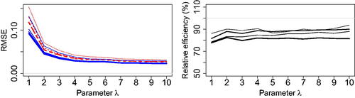
Table 1 Root mean squared error ($\times 100$) for the composite likelihood estimator $\hspace{0.17em}\log \hspace{0.17em}({\widehat{\lambda }}_{C;d})$ (left) with $d=2,3,4,5$ and cutoff distance $\delta =1,\sqrt{2},2$, and of the Vecchia likelihood estimator $\hspace{0.17em}\log \hspace{0.17em}({\widehat{\lambda }}_{V;d})$ (right) with $d=2,3,4,5$ and coordinate-based (p₁), random (p₂), middle out (p₃) and maximum–minimum (p₄) orderings.

	Composite estimator $\hspace{0.17em}\log \hspace{0.17em}({\widehat{\lambda }}_{C;d})$			Vecchia estimator $\hspace{0.17em}\log \hspace{0.17em}({\widehat{\lambda }}_{V;d})$
	cutoff distance δ			ordering
d	1	$\sqrt{2}$	2	p1	p2	p3	p4
2	3.08	3.43	3.86	3.34	3.93	3.56	4.54
3	—	3.08	3.34	2.82	3.05	2.83	3.18
4	—	2.93	3.17	2.79	2.81	2.77	2.87
5	—	—	3.31	2.69	2.71	2.68	2.70

NOTE: The Brown–Resnick model is here simulated with parameters σ = 10 and λ = 5 at D = 100 sites, with n = 100 replicates.

The computational time of each estimator is reported in Table 2. While the computational time for ${\widehat{\lambda }}_{C;d}$ grows fast as a function of the cutoff distance δ, it is essentially the same for each ordering considered for ${\widehat{\lambda }}_{V;d}$. Moreover, the computational time remains fairly moderate as d increases for ${\widehat{\lambda }}_{V;d}$, but it can be extremely large for ${\widehat{\lambda }}_{C;d}$ when d = 4, 5.

Table 2 Computational time (hr) for the composite likelihood estimator ${\widehat{\lambda }}_{C;d}$ (left) with $d=2,3,4,5$ and cutoff distance $\delta =1,\sqrt{2},2,\sqrt{5},\sqrt{8}$, and of the Vecchia likelihood estimator $\hspace{0.17em}\log \hspace{0.17em}({\widehat{\lambda }}_{V;d})$ (right) with $d=2,3,4,5$ and coordinate-based (p₁), random (p₂), middle out (p₃) and maximum–minimum (p₄) orderings.

	Composite estimator ${\widehat{\lambda }}_{C;d}$					Vecchia estimator ${\widehat{\lambda }}_{V;d}$
	cutoff distance δ					ordering
	1	$\sqrt{2}$	2	$\sqrt{5}$	$\sqrt{8}$	p1	p2	p3	p4
2	0.047	0.097	0.153	0.241${}^{\star }$	0.280${}^{\star }$	0.026	0.025	0.025	0.026
3	—	0.706	1.704	5.376${}^{\star }$	7.353${}^{\star }$	0.229	0.228	0.235	0.223
4	—	0.633	3.349	29.463${}^{\star }$	49.761${}^{\star }$	1.100	1.023	1.111	0.960
5	—	—	1.315	66.394${}^{\star }$	151.852${}^{\star }$	3.386	3.402	3.398	3.331

NOTE: The Brown–Resnick model is here simulated with parameters σ = 10 and λ = 5 at D = 100 sites, with n = 100 replicates. Numbers with an asterisk are extrapolated from the δ = 2 case by assuming that the computational time for ${\widehat{\lambda }}_{C;d}$ is proportional to the numbers reported in Table 1 of the supplementary materials.

Overall, when d = 2, the best solution is to use ${\widehat{\lambda }}_{C;d}$ but when d > 2 the best solution is to use ${\widehat{\lambda }}_{V;d}$ for reasons of both statistical efficiency and computational efficiency.

To investigate the scalability of the Vecchia likelihood estimator, we repeated our experiments for the Brown–Resnick model with parameters σ = 10 and λ = 5 in dimensions $D=25,49,100,144,225,400,625,1024$. Timing results reported in the supplementary materials demonstrate that, as expected, the computational time is linear in D, but it grows fast in d. In fact, the time is roughly proportional to the Bell number of order d (i.e., the cardinality of ${\mathcal{P}}_d$, the set of partitions of $\{1,\dots ,d\}$, recall (8)). Nevertheless, with moderate values of d, the linearity in D makes it possible to tackle high-dimensional extreme-value problems using the Vecchia likelihood estimator, while retaining fairly high efficiency.

Further simulations reported in the supplementary materials show that for the exchangeable logistic max-stable model, even more substantial gains in efficiency can be obtained with the Vecchia estimator. Moreover, when data are instead simulated in the max-domain of attraction of the logistic and Brown–Resnick models, the results are comparable, though the sub-asymptotic misspecification bias can in some cases be non-negligible and reduce the RMSE performance gap between the different estimators; see the supplementary materials.

4 Data Application

4.1 Red Sea Surface Temperature Dataset

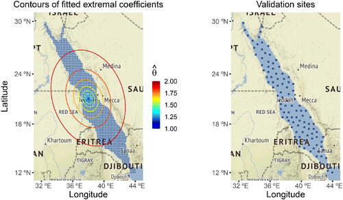
The spatial modeling of sea surface temperature (SST) extremes plays a key role in estimating changes in the Earth’s climate (Bulgin, Merchant, and Ferreira 2020) and understanding how ecosystems and marine life may be affected by global warming (Tittensor et al. 2021). While estimating marginal trends in SST observations is important for future predictions and risk planning and mitigation, characterizing their spatial tail dependence structure is needed to estimate extreme SST hotspots (Hazra and Huser 2021), and to assess the spatial extent of regions simultaneously affected by single extreme temperature events (see, e.g., Zhong, Huser, and Opitz 2022). In our real data application, we analyze (standardized) annual maxima of SST anomalies for the whole Red Sea, obtained on a fine grid of 1043 locations for 31 years from 1987 to 2015. The spatial grid is displayed in Figure 3. The Red Sea is a semi-enclosed sea with a very rich biodiversity, including abundant coral species that are often highly sensitive to modest SST increases. Before detailing our modeling of spatial extremal dependence, we first briefly summarize how the original data were pre-processed to obtain temperature anomalies, and how annual maxima were marginally standardized.

Fig. 3 Left: Map of the study domain, with the spatial grid (dots) covering the Red Sea at which SST data are available. Ellipses show contours of the fitted extremal coefficient function $\widehat{\theta }(\mathit{h})=1.1,\dots ,1.9$, with respect to the grid cell at the center, obtained by fitting the anisotropic Brown–Resnick max-stable model using the best Vecchia likelihood estimator. Right: Validation locations (dots) used in our cross-validation study.

The original data product was obtained from the Operational Sea Surface Temperature and Sea Ice Analysis (OSTIA; Donlon et al. 2012; see https://ghrsst-pp.metoffice.gov.uk/ostia-website/index.html), which produces satellite-derived daily SST measurements at a very high ${0.05}^{°}\times {0.05}^{°}$ spatial resolution; see Huser (2021) for a detailed exploratory analysis of this dataset, and Hazra and Huser (2021) for a comprehensive spatial analysis. In our study, we subsampled the spatial locations while still maintaining good spatial coverage (i.e., keeping every fourth longitude/latitude point), thus, yielding $11,315$ fields of D = 1043 highly spatially dependent daily observations. Because daily temperature data feature seasonality, and a possible time trend due to global warming, which also varies across space, it is therefore crucial to first detrend the marginal distributions and standardize them to a common scale, before modeling dependencies among SST extremes with a max-stable process. To estimate spatiotemporal trends (both in the mean and the variance of daily temperatures) in a very flexible way, we fitted a semiparametric normal model to all temperature observations within a certain radius of each spatial location, using a local likelihood approach. Then, after standardizing the data based on the fitted semiparametric model, we extracted annual maxima of SST anomalies and fitted a generalized extreme-value (GEV) distribution, which we then used to transform annual SST maxima to a common unit Fréchet scale by means of the probability integral transform. For further details on marginal modeling, see the supplementary materials.

In the next section, we model the dependence structure of the standardized annual maxima by fitting isotropic and anisotropic Brown–Resnick max-stable processes, and we focus on investigating differences between the performance of the traditional composite likelihood and the Vecchia likelihood approximation methods.

4.2 Dependence Modeling of the Red Sea Temperature Extremes

To fit the max-stable Brown–Resnick model, we first need to specify the variogram function Γ of the underlying Gaussian process $\epsilon (\mathit{s})$ in (9), which determines the form and range of dependencies that can be captured by the model. In our simulation study, we used a bounded variogram of the form $\Gamma (\mathit{h})=2{\sigma }^2\{1-\rho (\mathit{h})\}\le 2{\sigma }^2$, based on the stationary and isotropic exponential correlation function $\rho (\mathit{h})$, for comparison purposes with the Gaussian setting. Such a comparison is important to make sure the exact theoretical efficiency results in the Gaussian case (see the supplementary materials) can be generalized and carried over by analogy to the max-stable case (Section 3). However, using a bounded variogram also implies long-range dependence as the extremal coefficient is bounded away from independence at any spatial distance, that is, $\theta (\mathit{h})<2$. This is problematic in our data application, since we model SST anomaly maxima over a very large domain, namely the whole Red Sea, for which complete independence prevails at large distances. This suggests that we should use an unbounded variogram in our application. Moreover, given that the Red Sea has a geographically elongated shape, that it is only connected to the World Ocean through the artificial Suez canal in the North and the Gulf of Aden in the South, and because of the complex hydrodynamic patterns that these physical constraints entail, it makes sense to use an anisotropic variogram function. Therefore, the variogram model that we use here is $\Gamma ({\mathit{s}}_1,{\mathit{s}}_2)=\mathrm{E}\left[{\left\{\epsilon ({\mathit{s}}_1)-\epsilon ({\mathit{s}}_2)\right\}}^2\right]=2{(\sqrt{{({\mathit{s}}_1-{\mathit{s}}_2)}^{T}A({\mathit{s}}_1-{\mathit{s}}_2)}/\lambda )}^{\alpha }$, where $\lambda \in (0,\infty )$ is a range parameter, $\alpha \in (0,2)$ is a smoothness parameter, and A is the rotation matrix, which has the form $A=\left[\begin{array}{cc}\hspace{0.17em}\cos \hspace{0.17em}(\theta )& -\hspace{0.17em}\sin \hspace{0.17em}(\theta )\\ \hspace{0.17em}\sin \hspace{0.17em}(\theta )& \hspace{0.17em}\cos \hspace{0.17em}(\theta )\end{array}\right]\left[\begin{array}{cc}1& 0\\ 0& a\end{array}\right]\left[\begin{array}{cc}\hspace{0.17em}\cos \hspace{0.17em}(\theta )& \hspace{0.17em}\sin \hspace{0.17em}(\theta )\\ -\hspace{0.17em}\sin \hspace{0.17em}(\theta )& \hspace{0.17em}\cos \hspace{0.17em}(\theta )\end{array}\right]$, where $\theta \in (-\pi /2,\pi /2)$ is the rotation angle, and a > 0 determines the extent of anisotropy, with a = 1 corresponding to isotropy. The dependence parameter vector, $\mathit{\psi }$, thus, consists of four parameters, that is, $\mathit{\psi }={(\alpha ,\lambda ,a,\theta )}^{\top }\in \Psi =(0,2)\times {(0,\infty )}^2\times (-\pi /2,\pi /2)$.

To fit the Brown–Resnick model, we consider the (traditional) weighted composite likelihood method, as well as the proposed Vecchia likelihood approximation, which is expected to boost both the computational and statistical efficiency according to our theoretical and simulation results. For the composite likelihood method, we consider pairwise (d = 2) and triplewise (d = 3) likelihoods, but cannot consider higher values of d > 3 due to computational reasons. For each cutoff dimension d, we set binary weights $\mathbb{I}({\max }_{\{i,j\}}\Vert {\mathit{h}}_{\{i,j\}}\Vert \le \delta )$ with cutoff distance δ specified such that the resulting composite likelihood function contains m × D terms in total, where D = 1043 is the number of locations and $m=2,4,6,8$. Therefore, m = 2 roughly corresponds to including first-order neighbors only, m = 4 roughly corresponds to including second-order neighbors only, and so forth, though the complex Red Sea boundaries mean that a few additional higher-order neighbors (i.e., at slightly longer distances) may also be included. For the Vecchia likelihood approximation, we choose the cutoff dimensions $d=2,3,4,5$ and use the four orderings considered above, that is, coordinate-based (p₁), random (p₂), middle-out (p₃), and maximum–minimum (p₄).

Because the data are (approximately) gridded, there are only a few unique pairwise distances that characterize the likelihood contributions involved in the composite and Vecchia likelihoods. This, combined with the fact that SST maxima are highly spatially dependent, implies that the range λ and smoothness α may not be easily identifiable, and we have indeed found it difficult to estimate them both simultaneously. In our analysis, we thus fix the smoothness parameter to three representative values, that is, $\alpha =0.5$ (rough field), α = 1 (intermediate case, similar to a Brownian motion), and $\alpha =1.5$ (smooth field), then we estimate the parameter vector ${\mathit{\psi }}_{\alpha }={(\lambda ,a,\theta )}^{\top }$ by maximizing the composite and Vecchia likelihoods for fixed α, and subsequently select the best value of α by cross-validation.

An extensive cross-validation study is hence conducted to compare the goodness-of-fit and prediction performance of the different fitted models, obtained by (i) varying the value of $\alpha \in \{0.5,1,1.5\}$; (ii) considering the general anisotropic Brown–Resnick model or its isotropic restriction (with a = 1, θ = 0 fixed); and (iii) using different inference approaches (composite or Vecchia likelihoods under different settings). Precisely, we leave out a validation set consisting of about 10% of locations (i.e., exactly 105 out of 1043), selected as the last 10% of locations from the maximum-minimum ordering. This ensures that the validation locations are well spread-out throughout the whole Red Sea; see Figure 3. Then, we calculate the sum of the negative conditional log-density for each spatiotemporal point from the validation set, given the values at its four closest neighbors from the training set for the same temporal replicate. In other words, the (negative) log-score we consider is (11) $$S=-\sum _{i=1}^n\sum _{j\in \mathcal{V}}\hspace{0.17em}\log \hspace{0.17em}f(z_{i;j}|{\mathit{z}}_{i;\mathcal{T}(j)};{\widehat{\mathit{\psi }}}_{\alpha })$$(11) where $\mathcal{V}$ is the index set of validation locations, $\mathcal{T}(j)$ is the index set of the four closest training locations from the jth location ${\mathit{s}}_j$, ${\mathit{z}}_{i;\mathcal{T}(j)}$ is the corresponding observation vector from these neighboring locations from the training set, f is the Brown–Resnick density, and ${\widehat{\mathit{\psi }}}_{\alpha }$ is the estimated parameter vector (for fixed α), obtained for each inference method. Since we consider only four nearest neighbors to calculate the score (11), the densities involved are of maximum dimension five, which is still computationally feasible. We also stress that while (11) may seem to mimic the way the Vecchia likelihood is constructed, it does not give an unfair advantage to the latter, for two reasons: first and foremost, (11) is evaluated on a validation set, while the Vecchia likelihood estimator is computed based on a separate training set; and second, the conditional densities involved in (11) are very different from those included in the Vecchia likelihood, especially under random and maximum-minimum orderings (which do not order neighboring locations sequentially).

The cross-validation results are reported in Table 3. Strikingly, the Vecchia likelihood approximation is uniformly better than its composite likelihood counterpart, except in two cases (d = 2, $\alpha =1.5$, using random or maximum–minimum ordering), which give slightly worse results than the best composite likelihood estimator. Overall, the Vecchia likelihood estimator thus clearly outperforms the composite likelihood estimator by a large margin, whatever the ordering (for Vecchia estimators) and cutoff distance (for composite estimators). It is also interesting to note that composite methods in the isotropic case do not even find that α = 1 is better than $\alpha =0.5$, while all other cases give strong support for α = 1. Moreover, composite methods perform very poorly when $\alpha =1.5$, while the fits are much more reasonable for Vecchia methods, suggesting that composite methods are less reliable. In terms of computational time, reported in Table 4, the Vecchia likelihood estimator is also often much faster than the composite likelihood estimator for fixed d. In particular, the Vecchia likelihood estimator with d = 2 only takes a few minutes to run, and already outperforms the best traditional composite likelihood estimator in terms of its log score, even when d = 3. Moreover, the increase in computational cost as the cutoff dimension d increases is often very large for traditional composite likelihoods, but relatively moderate for the Vecchia likelihood approach. Hence, the Vecchia likelihood estimator is both statistically and computationally more efficient, and easy to implement, which provides strong support for using it in practice.

Table 3 Negative conditional log score S in (11) for each scenario based on a selection of 10% evenly spread validation locations.

	Vecchia					Composite
	Ordering	d = 2	d = 3	d = 4	d = 5	d = 2	d = 3	m
Anisotropic	p1	$97.6/92.5/107.7$	$96.6/91.6/107.1$	$97.7/91.4/113$	$98/91.4/112.7$	$130.1/\mathbf{115.9}/1053.6$	$125.8/117.6/946.3$	2
	p2	$101.4/93.2/118$	$97.7/91.6/105$	$100.6/91.4/105.5$	$97.3/91.5/105.1$	$129.8/117/1101.1$	$126/117/930.8$	4
	p3	$99.2/93.2/107$	$95.9/91.8/104.2$	$97.2/91.4/106.1$	$97.8/\mathbf{91.4}/105.2$	$129.7/117.4/1097.3$	$126.1/116.9/927.6$	6
	p4	$102.8/93.6/126.1$	$98/91.8/106.4$	$101.4/91.5/104.9$	$97.1/91.5/106.6$	$129.7/117.1/1061.7$	$126.3/116.9/929.5$	8
Isotropic	p1	$98/93.1/108.4$	$97.2/92.2/107$	$98.1/92/106.2$	$98.4/91.9/106.3$	$122.5/133.6/1088.4$	$\mathbf{117.7}/128.6/845.2$	2
	p2	$100.4/93/110.8$	$98.2/92.1/106.4$	$97.9/92/106.6$	$98.1/92/106.3$	$122.5/134.4/1101.6$	$117.7/128.4/841.4$	4
	p3	$98.1/93.2/108.1$	$96.5/92/106.9$	$97.5/\mathbf{91.9}/106.8$	$98.1/91.9/106.7$	$122.2/135.7/1124.6$	$117.8/128.4/840.4$	6
	p4	$101.7/92.8/114.4$	$98.5/92.2/106.8$	$97.6/92/106.6$	$97.9/92.1/107$	$122.3/135.8/1105.2$	$117.9/128.4/841.9$	8

NOTE: The three values in each cell correspond to $\alpha =0.5,1,1.5$, respectively. The best scenarios in each block (Vecchia/Composite × Anisotropic/Isotropic) are highlighted in bold. Orderings p₁, p₂, p₃, p₄ correspond to coordinate-based, random, middle-out, and maximum-minimum orderings, respectively. The maximum dimension of likelihood contributions is d (i.e., for Vecchia methods, with at most d–1 variables in the conditioning sets), and m relates to the cutoff distance for composite likelihoods.

Table 4 Computational time used in each scenario, measured in seconds.

	Vecchia					Composite
	Ordering	d = 2	d = 3	d = 4	d = 5	d = 2	d = 3	m
Anisotropic	p1	$201/24/120$	$1454/513/894$	$2790/2384/2051$	$6319/6699/9681$	$148/372/171$	$1266/1605/2304$	2
	p2	$329/155/152$	$796/469/527$	$1406/1703/2779$	$4796/6399/6928$	$573/377/335$	$2243/2442/3833$	4
	p3	$284/137/93$	$1026/459/868$	$3593/2245/2588$	$13670/5335/8566$	$480/548/565$	$3291/3381/3535$	6
	p4	$213/190/115$	$840/464/624$	$1836/2654/2330$	$9902/5032/7156$	$688/878/722$	$4972/4823/6493$	8
Isotropic	p1	$37/13/18$	$104/56/176$	$372/290/470$	$1136/829/1258$	$21/31/33$	$137/262/253$	2
	p2	$20/16/19$	$97/70/92$	$350/242/379$	$998/954/1056$	$39/56/58$	$417/452/462$	4
	p3	$19/13/30$	$97/73/84$	$340/273/414$	$1134/857/1442$	$55/81/90$	$501/613/623$	6
	p4	$19/12/18$	$101/62/84$	$370/218/332$	$1042/722/1179$	$69/100/108$	$560/937/843$	8

NOTE: For further details, see the caption of Figure 3.

Overall, our proposed inference approach based on the Vecchia approximation thus delivers excellent results. From Table 3, it is evident that the best results are obtained for α = 1, with moderate but visible improvements in the anisotropic case. In the best case (anisotropic model with α = 1, fitted using the Vecchia estimator with middle-out ordering and four conditioning sites, that is, d = 5), the parameter estimates are $\widehat{\lambda }=113.69$ km, $\widehat{a}=0.73$ and $\widehat{\theta }=0.40$, with 95% confidence intervals $\lambda \in (98.49,128.25),a\in (0.65,0.79)$, and $\theta \in (0.12,0.50)$, obtained from a parametric bootstrap with 300 bootstrap replicates. These confidence intervals are very similar to those obtained from the (computationally cheaper) jackknife method: $\lambda \in (96.85,130.54),a\in (0.66,0.80)$, and $\theta \in (0.29,0.51)$. The confidence intervals for a clearly exclude the value 1, suggesting the data are indeed anisotropic. Figure 3 displays the contours of the fitted bivariate extremal coefficient $\theta (\mathit{h})=1.1,\dots ,1.9$ with respect to the location at the center of the Red Sea, as described in (10), based on the best model. The elliptical shape of the estimated contours is well aligned with the geometry of the Red Sea, with stronger dependence along its main axis, which is physically meaningful.

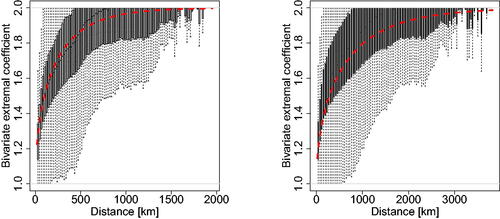
To further compare the Vecchia and composite likelihood approaches, we study the goodness-of-fit of the best-fitting models in each case by comparing the estimated bivariate extremal coefficients, binned by distance class, with their empirical counterparts. Figure 4 shows the estimated extremal coefficients, plotted as a function of the Mahalanobis distance $d({\mathit{s}}_1,{\mathit{s}}_2)=\sqrt{{({\mathit{s}}_1-{\mathit{s}}_2)}^T\widehat{A}({\mathit{s}}_1-{\mathit{s}}_2)}$ where $\widehat{A}$ is the estimated rotation matrix, for the best anisotropic models obtained using the Vecchia and composite approaches. While the model fitted using the Vecchia method captures the spatial extremal dependence very well at all distances, the fit is quite poor when using the composite likelihood approach, especially at moderately long distances. This strongly reinforces the benefits of using the Vecchia likelihood estimator.

Fig. 4 Binned bivariate empirical extremal coefficients (boxplots), plotted as a function of the Mahalanobis distance $d({\mathit{s}}_1,{\mathit{s}}_2)$, and their model-based counterparts (dashed curves) for the best anisotropic models obtained using the Vecchia likelihood approach (left) and traditional composite likelihood approach (right). The settings of these four “best models” can be read from Table 3.

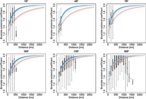
We then also compare the performance of the best anisotropic models (for both Vecchia and composite likelihood approaches) by comparing empirical and fitted extremal coefficients along different directions, and for sub-datasets of different sizes. Specifically, in order to verify the stability of the fitted models, we fit them again using (approximately) 50%, 25%, 12.5%, and 6.25% spread-out sites, chosen according to the maximum–minimum ordering, among the 1043 sites from the complete dataset. Figure 5 shows plots of the estimated bivariate coefficients for direction-specific pairs of sites in the different sub-panels, plotted against the Euclidean distance between sites. More precisely, binned empirical estimates are compared with model-based estimates for 12 prevailing directions, namely ${15}^{°},{30}^{°},\dots ,{165}^{°}$ (from the East direction in a counterclockwise manner). Figure 4 shows the results for six selected directions, and the supplementary materials show the full results. Again, the Vecchia likelihood estimator is able to deliver good and consistent performances in all cases, while the composite likelihood estimator fails completely for some specific directions (see, e.g., the panels corresponding to ${15}^{°}$ or ${75}^{°}$). These differences prove the superiority of the Vecchia method when compared to traditional composite likelihood methods.

Fig. 5 Binned empirical extremal coefficients (boxplots) and their model-based counterparts (curves) for different directions, that is, ${15}^{°},{45}^{°},\dots ,{165}^{°}$ (subpanels from top left to bottom right), computed by fitting the best anisotropic models obtained with the Vecchia method (solid curves) and the composite likelihood method (dashed curves) based on sub-datasets of size $1,1/2,1/4,1/8,1/16\times 100\%$ of the complete dataset (light to dark). The different shades of gray of the binned boxplots correspond to the number of data points used in each boxplot, with darker gray corresponding to more points.

Implications of our results include that the Vecchia method is able to better capture the anisotropic dependence structure of our Red Sea data, especially in certain directions. Better models might in turn yield more accurate simulations and better risk assessment of future spatial extreme events. In future research, it would be interesting to conduct a rigorous risk assessment of Red Sea surface temperature extremes using the Vecchia method and to study their impact in a changing climate.

5 Conclusion

In this article, we have proposed a new fast and efficient inference method for max-stable processes based on the Vecchia likelihood approximation, which significantly outperforms traditional composite likelihood methods. Unlike pairwise likelihood methods proposed originally by Padoan, Ribatet, and Sisson (2010) and later extended to higher-order truncated composite likelihoods by Castruccio, Huser, and Genton (2016) and others, the Vecchia method provides a valid likelihood approximation (i.e., it is itself the likelihood of a well-defined approximated process), thus, giving theoretical guarantees to provide improved results, and the number of lower-dimensional likelihood terms involved in it remains linear in the data dimension D. Moreover, while it is difficult to choose the cutoff distance δ and the cutoff dimension d optimally in truncated composite likelihoods, the performance of the Vecchia likelihood estimator is often only moderately sensitive to the choice of the permutation, and always improves as d increases in the settings we have investigated. Therefore, overall, the Vecchia approximation method is uniformly better than traditional truncated composite likelihoods, be it in terms of statistical efficiency, computational efficiency, ease of implementation, and tuning of parameters. We verified this conclusion in various settings, based on (i) theoretical asymptotic relative efficiency calculations in the case of Gaussian processes, (ii) extensive simulations in the case of max-stable processes, as well as (iii) a substantial real data application to sea surface temperature extremes measured over the whole Red Sea at more than a thousand sites. Our results thus suggest that the superiority of the Vecchia likelihood estimator holds more generally and can be applied in other spatial contexts where the likelihood function is intractable or difficult to evaluate in high dimensions. While the cutoff dimension d cannot be too big for popular max-stable processes such as the Brown–Resnick model, we have found that the Vecchia approximation method already provides satisfactory results for relatively small d, for example, d = 3 or 4, providing a good tradeoff between computational and statistical efficiency and major improvements compared to the pairwise likelihood case with d = 2. In future research, it would be interesting to investigate how the Vecchia and composite likelihood approaches compare when there are missing values under various missingness mechanisms (e.g., missing-at-random, missing-in-a-block, etc.).

Supplementary Materials

PDF Supplement: This supplement contains the proof that the Vecchia estimator is monotonically improving as d increases; theoretical results on the asymptotic relative efficiency of Vecchia, modified Vecchia, and composite likelihood estimators in the Gaussian case; and further results in the max-stable case (PDF file)

R Code: This supplement contains the code to implement the Vecchia, traditional composite, and full likelihood estimators for the Brown–Resnick model, as well as a small simulation example (zip file). The code script files for the application and necessary data files have been packaged in the GitHub repository of the third author; see https://github.com/PangChung/VecchiaSpatialExtremes

Acknowledgments

The authors would like to gratefully thank the Editor, Associate Editor, and two anonymous reviewers for their constructive comments and suggestions that helped improve the quality of the article.

Disclosure Statement

No potential competing interest was reported by the author(s).

Additional information

Funding

Work by Raphaël Huser and Peng Zhong in this publication was supported by the King Abdullah University of Science and Technology (KAUST) Office of Sponsored Research (OSR) under Awards No. OSR-CRG2017-3434 and No. OSR-CRG2020-4394. Part of the effort of Michael L. Stein is based on work supported by the U.S. Department of Energy, Office of Science, Office of Advanced Scientific Computing Research (ASCR) under Contract DE-AC02-06CH11347.

References

- Beranger, B., Stephenson, A. G., and Sisson, S. A. (2021), “High-Dimensional Inference Using the Extremal Skew-t Process,” Extremes, 24, 653–685. DOI: 10.1007/s10687-020-00376-1.
- Bopp, G., Shaby, B. A., and Huser, R. (2021), “A Hierarchical Max-Infinitely Divisible Spatial Model for Extreme Precipitation,” Journal of American Statistical Association, 116, 93–106. DOI: 10.1080/01621459.2020.1750414.
- Bulgin, C. E., Merchant, C. J., and Ferreira, D. (2020), “Tendencies, Variability and Persistence of Sea Surface Temperature Anomalies,” Scientific Reports, 10, 7986. DOI: 10.1038/s41598-020-64785-9.
- de Carvalho, M., and Davison, A. C. (2014), “Spectral Density Ratio Models for Multivariate Extremes,” Journal of the American Statistical Association, 109, 764–776. DOI: 10.1080/01621459.2013.872651.
- Castruccio, S., Huser, R., and Genton, M. G. (2016), “High-Order Composite Likelihood Inference for Max-Stable Distributions and Processes,” Journal of Computational and Graphical Statistics, 25, 1212–129. DOI: 10.1080/10618600.2015.1086656.
- Davis, R. A., Küppelberg, C., and Steinkohl, C. (2013), “Max-Stable Processes for Modeling Extremes Observed in Space and Time,” Journal of the Korean Statistical Society, 42, 399–414. DOI: 10.1016/j.jkss.2013.01.002.
- Davison, A. C., and Huser, R. (2015), “Statistics of Extremes,” Annual Review of Statistics and its Application, 2, 203–235. DOI: 10.1146/annurev-statistics-010814-020133.
- Davison, A. C., Huser, R., and Thibaud, E. (2019), “Spatial Extremes,” in: Handbook of Environmental and Ecological Statistics, eds. A. E. Gelfand, M. Fuentes, J. A. Hoeting, and R. L. Smith, pp. 711–744, Boca Raton, FL: CRC Press.
- Davison, A. C., Padoan, S., and Ribatet, M. (2012), “Statistical Modelling of Spatial Extremes,” (with Discussion), Statistical Science, 27, 161–186. DOI: 10.1214/11-STS376.
- de Fondeville, R., and Davison, A. C. (2018), “High-Dimensional Peaks-Over-Threshold Inference,” Biometrika, 105, 575–592. DOI: 10.1093/biomet/asy026.
- de Haan, L. (1984), “A Spectral Representation for Max-Stable Processes,” Annals of Probability, 12, 1194–1204.
- Dombry, C., Engelke, S., and Oesting, M. (2017), “Bayesian Inference for Multivariate Extreme Value Distributions,” Electronic Journal of Statistics, 11, 4813–4844. DOI: 10.1214/17-EJS1367.
- Donlon, C. J., Martin, M., Stark, J., Roberts-Jones, J., Fiedler, E., and Wimmer, W. (2012), “The Operational Sea Surface Temperature and Sea Ice Analysis (OSTIA) System,” Remote Sensing of Environment, 116, 140–158. DOI: 10.1016/j.rse.2010.10.017.
- Einmahl, J. H. J., Kiriliouk, A., Krajina, A., and Segers, J. (2016), “An M-estimator of Spatial Tail Dependence,” Journal of the Royal Statistical Society, Series B, 78, 275–298. DOI: 10.1111/rssb.12114.
- Engelke, S., and Hitz, A. S. (2020), “Graphical Models for Extremes,” (with Discussion), Journal of the Royal Statistical Society, Series B, 82, 871–932. DOI: 10.1111/rssb.12355.
- Engelke, S., and Ivanovs, J. (2021), “Sparse Structures for Multivariate Extremes,” Annual Review of Statistics and its Application, 8, 241–270. DOI: 10.1146/annurev-statistics-040620-041554.
- Fraser, D. A. S., and Reid, N. (2020), “Combining Likelihood and Significance Functions,” Statistica Sinica, 30, 1–15. DOI: 10.5705/ss.202016.0508.
- Genton, M. G., Ma, Y., and Sang, H. (2011), “On the Likelihood Function of Gaussian Max-Stable Processes,” Biometrika, 98, 481–488. DOI: 10.1093/biomet/asr020.
- Guinness, J. (2018), “Permutation and Grouping Methods for Sharpening Gaussian Process Approximations,” Technometrics, 60, 415–429. DOI: 10.1080/00401706.2018.1437476.
- Gumbel, E. J. (1960), “Distributions de valeurs extrêmes en plusieurs dimensions,” Publication de l’Institut de Statistique de l’Universié de Paris, 9, 171–173.
- Gumbel, E. J. (1961), “Bivariate Logistic Distributions,” Journal of the American Statistical Association, 56, 335–349. DOI: 10.1080/01621459.1961.10482117.
- Hazra, A., and Huser, R. (2021), “Estimating High-Resolution Red Sea Surface Temperature Hotspots, Using a Low-Rank Semiparametric Spatial Model,” Annals of Applied Statistics, 15, 572–596.
- Huser, R. (2013), “Statistical Modeling and Inference for Spatio-Temporal Extremes,” Ph.D. thesis, École Polytechnique Fédérale de Lausanne.
- ——- (2021), “Editorial: EVA 2019 Data Competition on Spatio-Temporal Prediction of Red Sea Surface Temperature Extremes,” Extremes, 24, 91–104.
- Huser, R., and Davison, A. C. (2013), “Composite Likelihood Estimation for the Brown–Resnick Process,” Biometrika, 100, 511–518. DOI: 10.1093/biomet/ass089.
- ——- (2014), “Space-Time Modelling of Extreme Events,” Journal of the Royal Statistical Society, Series B, 76, 439–461.
- Huser, R., Davison, A. C., and Genton, M. G. (2016), “Likelihood Estimators for Multivariate Extremes,” Extremes, 19, 79–103. DOI: 10.1007/s10687-015-0230-4.
- Huser, R., Dombry, C., Ribatet, M., and Genton, M. G. (2019), “Full Likelihood Inference for Max-Stable Data,” Stat, 8, e218. DOI: 10.1002/sta4.218.
- Huser, R., and Genton, M. G. (2016), “Non-Stationary Dependence Structures for Spatial Extremes, Journal of Agricultural, Biological and Environmental Statistics, 21, 470–491. DOI: 10.1007/s13253-016-0247-4.
- Hüsler, J., and Reiss, R. D. (1989), “Maxima of Normal Random Vectors: Between Independence and Complete Dependence,” Statistics & Probability Letters, 7, 283–286. DOI: 10.1016/0167-7152(89)90106-5.
- Kabluchko, Z., Schlather, M., and de Haan, L. (2009), “Stationary Max-Stable Fields Associated to Negative Definite Functions,” Annals of Probability, 37, 2042–2065.
- Katzfuss, M., and Guinness, J. (2021), “A General Framework for Vecchia Approximations of Gaussian Processes,” Statistical Science, 36, 124–141. DOI: 10.1214/19-STS755.
- Katzfuss, M., Guinness, J., Gong, W., and Zilber, D. (2020), “Vecchia Approximations of Gaussian-Process Predictions,” Journal of Agricultural, Biological and Environmental Statistics, 25, 383–414. DOI: 10.1007/s13253-020-00401-7.
- Lenzi, A., Bessac, J., Rudi, J., and Stein, M. L. (2023), “Neural Networks for Parameter Estimation in Intractable Models,” Computational Statistics and Data Analysis, 185, 107762. DOI: 10.1016/j.csda.2023.107762.
- Lindgren, F., Rue, H., and Lindström, J. (2011), “An Explicit Link between Gaussian Fields and Gaussian Markov Random Fields: The Stochastic Partial Differential Equation Approach,” Journal of the Royal Statistical Society, Series B, 73, 423–498. DOI: 10.1111/j.1467-9868.2011.00777.x.
- Nascimento, M., and Shaby, B. A. (2022), “A Vecchia Approximation for High-Dimensional Gaussian Cumulative Distribution Functions Arising from Spatial Data,” Journal of Statistical Computation and Simulation, 92, 1977–1994. DOI: 10.1080/00949655.2021.2016759.
- Opitz, T. (2013), “Extremal t Processes: Elliptical Domain of Attraction and a Spectral Representation,” Journal of Multivariate Analysis, 122, 409–413. DOI: 10.1016/j.jmva.2013.08.008.
- Pace, L., Salvan, A., and Sartori, N. (2019), “Efficient Composite Likelihood for a Scalar Parameter of Interest,” Stat, 8, e222. DOI: 10.1002/sta4.222.
- Padoan, S. A., Ribatet, M., and Sisson, S. A. (2010), “Likelihood-based Inference for Max-Stable Processes,” Journal of the American Statistical Association, 105, 263–277. DOI: 10.1198/jasa.2009.tm08577.
- Papastathopoulos, I., and Strokorb, K. (2016), “Conditional Independence among Max-Stable Laws,” Statistics & Probability Letters, 108, 9–15. DOI: 10.1016/j.spl.2015.08.008.
- Reich, B. J., and Shaby, B. A. (2012), “A Hierarchical Max-Stable Spatial Model for Extreme Precipitation,” Annals of Applied Statistics, 6, 1430–1451. DOI: 10.1214/12-AOAS591.
- Rue, H., and Held, L. (2005), Gaussian Markov Random Fields: Theory and Applications, Monographs on Statistics and Applied Probability (Vol. 104), London: Chapman & Hall.
- Sainsbury-Dale, M., Zammit-Mangion, A., and Huser, R. (2023), “Likelihood-Free Parameter Estimation with Neural Bayes Estimators,” The American Statistician, to appear. DOI: 10.1080/00031305.2023.2249522.
- Sang, H., and Genton, M. G. (2014), “Tapered Composite Likelihood for Spatial Max-Stable Models,” Spatial Statistics, 8, 86–103. DOI: 10.1016/j.spasta.2013.07.003.
- Schäfer, F., Katzfuss, M., and Owhadi, H. (2021), “Sparse Cholesky Factorization by Kullback–Leibler Minimization,” SIAM Journal on Scientific Computing, 43, A2019–A2046. DOI: 10.1137/20M1336254.
- Segers, J. (2012), “Max-Stable Models for Multivariate Extremes,” REVSTAT. 10, 61–82.
- Shi, D. (1995), “Fisher Information for a Multivariate Extreme Value Distribution,” Biometrika, 82, 644–649. DOI: 10.1093/biomet/82.3.644.
- Stein, M. L., Chi, Z., and Welty, L. J. (2004), “Approximating Likelihoods for Large Spatial Data Sets,” Journal of the Royal Statistical Society, Series B, 66, 275–296. DOI: 10.1046/j.1369-7412.2003.05512.x.
- Stephenson, A., and Tawn, J. A. (2005), “Exploiting Occurrence Times in Likelihood Inference for Componentwise Maxima,” Biometrika, 92, 213–227. DOI: 10.1093/biomet/92.1.213.
- Stephenson, A. G., Shaby, B. A., Reich, B. J., and Sullivan, A. L. (2015), “Estimating Spatially Varying Severity Thresholds of a Forest Fire Danger Rating System Using Max-Stable Extreme-Event Modeling,” Journal of Applied Meteorology and Climatology, 54, 395–407. DOI: 10.1175/JAMC-D-14-0041.1.
- Thibaud, E., Aalto, J., Cooley, D. S., Davison, A. C., and Heikkinen, J. (2016), “Bayesian Inference for the Brown–Resnick Process, with an Application to Extreme Low Temperatures,” Annals of Applied Statistics, 10, 2303–2324.
- Tittensor, D. P., Novaglio, C., Harrison, C. S., Heneghan, R. F., Barrier, N., Bianchi, D., et al. (2021), “Next-Generation Ensemble Projections Reveal Higher Climate Risks for Marine Ecosystems,” Nature Climate Change, 11, 973–981. DOI: 10.1038/s41558-021-01173-9.
- Varin, C., Reid, N., and Firth, D. (2011), “An Overview of Composite Likelihood Methods,” Statistica Sinica, 21, 5–42.
- Vecchia, A. V. (1988), “Estimation and Model Identification for Continuous Spatial Processes,” Journal of the Royal Statistical Society, Series B, 50, 297–312. DOI: 10.1111/j.2517-6161.1988.tb01729.x.
- Vettori, S., Huser, R., and Genton, M. G. (2019), “Bayesian Modeling of Air Pollution Extremes Using Nested Multivariate Max-Stable Processes,” Biometrics, 75, 831–841. DOI: 10.1111/biom.13051.
- Vettori, S., Huser, R., Segers, J., and Genton, M. G. (2020), “Bayesian Model Averaging Over Tree-based Dependence Structures for Multivariate Extremes,” Journal of Computational and Graphical Statistics, 29, 174–190. DOI: 10.1080/10618600.2019.1647847.
- Wadsworth, J. L. (2015), “On the Occurrence Times of Componentwise Maxima and Bias in Likelihood Inference for Multivariate Max-Stable Distributions,” Biometrika, 102, 705–711. DOI: 10.1093/biomet/asv029.
- Wadsworth, J. L., and Tawn, J. A. (2014), “Efficient Inference for Spatial Extreme Value Processes Associated to Log-Gaussian Random Functions,” Biometrika, 101, 1–15. DOI: 10.1093/biomet/ast042.
- Whitaker, T., Beranger, B., and Sisson, S. A. (2020), “Composite Likelihood Methods for Histogram-Valued Random Variables,” Statistics and Computing, 30, 1459–1477. DOI: 10.1007/s11222-020-09955-5.
- Zhong, P., Huser, R., and Opitz, T. (2022), “Modeling Non-stationary Temperature Maxima based on Extremal Dependence Changing with Event Magnitude,” Annals of Applied Statistics, 16, 272–299.