A distribution-free method for change point detection in non-sparse high dimensional data

Abstract

We propose a distribution-free distance-based method for high dimensional change points that can address challenging situations when the sample size is very small compared to the dimension as in the so-called HDLSS data or when non-sparse changes may occur due to change in many variables but with small significant magnitudes. Our method can detect changes in mean or variance of high dimensional observations as well as other distributional changes. We present efficient algorithms that can detect single and multiple high dimensional change points. We use nonparametric metrics, including a new dissimilarity measure and some new distance and difference distance matrices, to develop a procedure to estimate change point locations. We also introduce a nonparametric test to determine the significance of estimated change points. We provide theoretical guaranties for our method and demonstrate its empirical performance in comparison with some of the recent methods for high dimensional change points. An R package called HDDchangepoint is developed to implement the proposed method.

Keywords:

• Difference distance matrix
• Dissimilarity measure
• High dimensional change point
• High dimensional data
• Wild binary segmentation

Disclaimer

As a service to authors and researchers we are providing this version of an accepted manuscript (AM). Copyediting, typesetting, and review of the resulting proofs will be undertaken on this manuscript before final publication of the Version of Record (VoR). During production and pre-press, errors may be discovered which could affect the content, and all legal disclaimers that apply to the journal relate to these versions also.

1 Introduction

Change point analysis is frequently used in various fields such as economics, finance, engineering, genetics and medical research. The main objective is to detect significant changes in the underlying distribution of a data sequence. The change point problem is well studied for low dimensional data in the literature, however change point analysis is challenging for high dimensional data which are growing in different domains. A change could happen in a small or large subset of the variables and with a small or large magnitude, but when the sample size is small compared to the number of variables it is difficult to distinguish a significant change point from just random variability.

In recent years there has been increasing interest in the so-called high-dimensional low-sample-size (HDLSS) data where the sample size n is very small while the dimension p can be very large. The asymptotics for HDLSS data is different than the usual high dimensional asymptotic setting (i.e., $p>n\to \infty$) in the sense that $p\to \infty$ but the sample size n can remain fixed (e.g., Hall et al., 2005; Jung and Marron, 2009; Li, 2020). Detecting change points is more challenging for HDLSS data with small samples. In this paper, we will see that recent methods for high dimensional change points struggle to have a good performance with HDLSS data where sample size is very small compared to dimension.

A common strategy in the literature of high dimensional change points is to simplify the problem by reducing the dimension of data so a simpler algorithm such as a univariate change point algorithm can be applied to the transformed data. This may be done using random projection (e.g., Wang and Samworth, 2018; Hahn et al., 2020), geometric mapping (e.g., Grundy et al., 2020) or any other relevant techniques such as principal components (e.g., Xiao et al., 2019), factor analysis (e.g., Barigozzi et al., 2018) and regularisation approaches (e.g., Lee et al., 2016; Safikhani and Shojaie, 2022). This strategy relies on sparsity, often a significant amount of sparsity, to maintain its oracle performance. Such techniques may not be suitable for non-sparse change point problems. By non-sparse change points, we mean the changes that can happen in many variables and with small significant magnitudes.

Another strategy is to search for change point locations through dissimilarity distances between pairs of observations. This may be done using appropriate dissimilarity measures such as the interpoint distances (e.g., Li, 2020) or the divergence measures based on Euclidean distance (e.g., Matteson and James, 2014). Some authors including Garreau and Arlot (2018) and Chu and Chen (2019) indirectly use interpoint distances to develop methods based on counting the number of edges from a certain similarity graph constructed from interpoint distances. The performance, especially power, of such methods generally depends on distance measures and test statistics used, as also discussed in Li (2020). In this paper, we aim to develop a novel powerful method for detecting high dimensional change points based on dissimilarity measures, especially suitable for HDLSS data.

There has been a growing literature on change point analysis for high dimensional data in recent years. We review some of the recent methods focusing on offline change point detection. Chen and Zhang (2015), Garreau and Arlot (2018) and Chu and Chen (2019) developed change-point detection methods using kernels and similarity graphs. Wang and Samworth (2018) proposed a two-stage procedure called inspect for estimation of change points, which is based on random projection and sparsity. Their approach assumes the mean structure changes in a sparse subset of the variables and requires the normality assumption. Enikeeva and Harchaoui (2019) suggested a method for detecting a sparse change in mean in a sequence of high dimensional vectors. This method was studied for a single change point detection and was developed based on the normality assumption. Grundy et al. (2020) used geometric mapping to project the high dimensional data to two dimensions, namely distances and angles. Their approach requires the normality assumption. Liu et al. (2020) developed a general data-adaptive framework by extending the classical CUSUM statistic to construct a U-statistic-based CUSUM matrix. Their approach is based on the independence assumption for variables and is mainly studied for single change point detection. Li (2020) proposed an asymptotic distribution-free distance-based procedure for change point detection in high dimensional data. Using the random projection approach of Wang and Samworth (2018), Hahn et al. (2020) proposed a Bayesian algorithm to efficiently estimate the projection direction for change point detection. Yu and Chen (2021) established a bootstrap CUSUM test for finite sample change point inference in high dimensions. Follain et al. (2022) extended the random projection approach to estimate change points with heterogeneous missingness. There have also been a few other methods, some of which are reviewed in Liu et al. (2022).

Below we highlight the importance of our work and summarise our main contributions.

1. Change point detection for HDLSS data, when the sample size is very small, is challenging and understudied. Also, many of the existing methods focused on sparse change points (e.g., Wang and Samworth, 2018; Enikeeva and Harchaoui, 2019; Follain et al., 2022). Our method can deal with non-sparse high dimensional situations. Unlike existing methods which mainly detect changes in mean of high dimensional observations, our method can detect changes in mean or variance of observations and other distributional changes.

2. Unlike most of the recent methods for high dimensional change point detection which require the normality assumption as reviewed above, our approach does not require normality or any other distribution for variables. We use novel nonparametric tools to develop a method to detect change point locations.

3. Many of the recent methods in the literature either used a bootstrap/permutation procedure or derived asymptotic distribution to test significance of change points (e.g., Wang and Samworth, 2018; Yu and Chen, 2021). We establish both asymptotic and permutation procedures for our method to handle both small and large sample size situations.

4. Our strategy is to search for change point locations through an n × n matrix of distances instead of the n × p matrix of observations. Because the n × n matrix of distances has a smaller dimension which does not grow with p, it would be easier mathematically and computationally to investigate the distance matrix for a change point location.

We use the following notation throughout the paper. For a vector $\mathit{u}\in {ℝ}^p$, we write the L_q -norm as $\mathrm{\Vert }\mathit{u}{\mathrm{\Vert }}_q={({\sum }_{j=1}^p|{\mathit{u}}_j{|}^q)}^{1/q}$. The infinity norm is defined as $\mathrm{\Vert }\mathit{u}{\mathrm{\Vert }}_{\infty }={\max }_j\left|{\mathit{u}}_j\right|$. We write $\surd$ as the short version of square root. For a real-value constant a, notation $\left|a\right|$ denotes the absolute value of a, while for a set C, $\left|C\right|$ denotes the cardinality of C. Also, $O(.)$ and $o(.)$ denote the usual big O and little o notation. We sometimes write $O^p(.)$ or $o^p(.)$ to emphasise them for $p\to \infty$. We write $O_P(.)$ and $o_P(.)$ to denote, respectively, the big O in probability and the little o in probability. We use $\stackrel{P}{\to }$ and $\stackrel{D}{\to }$ for convergence in probability and convergence in distribution, respectively. We also define some more specific notation as we develop the paper.

2 Methodology

Let ${\mathit{X}}_1,{\mathit{X}}_2,\dots ,{\mathit{X}}_n$ be a sequence of independent p-dimensional random vectors with unknown probability distributions $F_1,F_2,\dots ,F_n$, respectively. In high dimensional settings we have $p\gg n$ and that the p variables in each observation ${\mathit{X}}_i=({\mathit{X}}_{i1},{\mathit{X}}_{i2},\dots ,{\mathit{X}}_{ip})$ are potentially correlated. We aim to develop a distribution-free approach, so we do not assume a parametric form for the distributions $F_1,F_2,\dots ,F_n$.

For the sake of clarity, we first present the proposed approach for detecting a single change point in high dimensions and then extend the idea for multiple change point detection in Section 3. The problem of detecting a single change point in general can be formulated as the following hypothesis testing problem(1) $$\{\begin{array}{c}{H}_0:F_1=F_2=\dots =F_n\hfill \\ H_1^s:F_1=\dots =F_{\tau -1}\ne F_{\tau }=\dots =F_n,\hfill \end{array}$$(1) where τ is a change point location, which is unknown too. When conducting this single change point problem, we first estimate the change point location τ and then test for significance of the estimated change point.

Let $\mathit{X}={[{\mathit{X}}_1,{\mathit{X}}_2,\dots ,{\mathit{X}}_n]}^T$ represent the entire data as an n × p matrix. As discussed in the introduction, the problem of change point detection in high dimensional situations is challenging, especially when n is very small compared to p. In our approach, instead of searching in the n × p space, we translate the problem into the lower dimensional space n × n without reducing the dimension of data. This is different than the dimensionality reduction techniques such as random projection (e.g., Wang and Samworth, 2018), geometric mapping (e.g., Grundy et al., 2020), principal components (e.g., Xiao et al., 2019) and factor analysis (e.g., Barigozzi et al., 2018) which reduce the dimension of data. We propose a distance-based method based on dissimilarity measures to find the change point location in the original data $\mathit{X}$ through the distance matrix of $\mathit{X}$. The dimension of the observed data $\mathit{X}$ is n × p while the dimension of its distance matrix is n × n, so it is easier mathematically and computationally to investigate the distance matrix for a change point location as n is small compared to p in high dimensions, especially in HDLSS data. We describe the idea in the sequel.

Let $d_{ij}:=d({\mathit{X}}_i,{\mathit{X}}_j)$ be a dissimilarity distance between observations ${\mathit{X}}_i$ and ${\mathit{X}}_j$, where $d(·,·)$ is a suitable dissimilarity distance function for high dimensional vectors. Since our proposal can be implemented with any suitable dissimilarity distance, we discuss the choice of dissimilarity distance measure after illustrating the main mechanism. We use the dissimilarity measure d_ij to obtain the n × n distance matrix between all pairs of the observations ${\mathit{X}}_1,{\mathit{X}}_2,\dots ,{\mathit{X}}_n$ as follows$$D=\left[\begin{array}{cccc}{d}_{11}& d_{12}& \dots & d_{1n}\\ ⋮& ⋮& \ddots & ⋮\\ d_{n1}& d_{n2}& \dots & d_{nn}\end{array}\right],$$in which $d_{11}=\dots =d_{nn}=0$.

To find the location of change point τ, we propose a procedure that finds an estimate of τ by finding the maximum distance between observations in the distance matrix D. For this, we define the distance difference between each pair of the observations as$$\begin{array}{cccc}& {\Delta }_{ij}:=|d_{ij}-d_{i,j-1}|,& i& =1,\dots ,n,j=2,\dots ,n\\ & {\Delta }_{i1}:=0,& i& =1,\dots ,n.\end{array}$$

This gives the following n × n matrix of distance differences, which we call difference distance matrix,$$\Delta =\left[\begin{array}{ccccc}0& {\Delta }_{12}& \dots & {\Delta }_{1,n-1}& {\Delta }_{1n}\\ ⋮& ⋮& \ddots & ⋮& ⋮\\ 0& {\Delta }_{n2}& \dots & {\Delta }_{n,n-1}& {\Delta }_{nn}\end{array}\right].$$

We then suggest an estimate of the change point location τ, based on the difference distance matrix Δ, as follows(2) $$\widehat{\tau }=\text{arg}\hspace{0.17em}{\max }_{1\le j\le n}\left\{\frac{1}{n}\sum _{i=1}^n{\Delta }_{ij}\right\}.$$(2)

The change point estimate $\widehat{\tau }$ is the location of maximum slope among the column sums of the difference distance matrix Δ (a simple illustrative example will be given later in Figure 1). If $\frac{1}{n}{\sum }_{i=1}^n{\Delta }_{ij}=0$ for all $j=1,\dots ,n$ or if they all are equal, then we set $\widehat{\tau }=\varnothing$, where the empty set $\varnothing$ means no change point is detected.

It is known that the Euclidean distance is not appropriate for high dimensional situations. A modified version of Euclidean distance can be obtained by dividing it by $\surd p$ for convergence guarantees in high dimensions, as suggested by Hall et al. (2005). One can use the modified Euclidean distance $d_{ij}=d({\mathit{X}}_i,{\mathit{X}}_j)=p^{-1/2}\mathrm{\Vert }{\mathit{X}}_i-{\mathit{X}}_j{\mathrm{\Vert }}_2$ or other L_q -norm distances in our approach. However, a more general dissimilarity measure that takes into account the information of distances from all the n – 2 other observations can be defined as(3) $$d_{ij}=d({\mathit{X}}_i,{\mathit{X}}_j)=\frac{1}{n-2}\sum _{l\ne i,j}|\mathrm{\Vert }{\mathit{X}}_i-{\mathit{X}}_l{\mathrm{\Vert }}_D-\mathrm{\Vert }{\mathit{X}}_j-{\mathit{X}}_l{\mathrm{\Vert }}_D|,$$(3) where $\mathrm{\Vert }·-·{\mathrm{\Vert }}_D$ can be any appropriate distance function. We here suggest two simple options for this. A natural multivariate option is to use the modified Euclidean distance function $\mathrm{\Vert }{\mathit{X}}_u-{\mathit{X}}_l{\mathrm{\Vert }}_D=p^{-1/2}\mathrm{\Vert }{\mathit{X}}_u-{\mathit{X}}_l{\mathrm{\Vert }}_2$ or modified L₁-norm $\mathrm{\Vert }{\mathit{X}}_u-{\mathit{X}}_l{\mathrm{\Vert }}_D=p^{-1}\mathrm{\Vert }{\mathit{X}}_u-{\mathit{X}}_l{\mathrm{\Vert }}_1$. A univariate option is to use a distance function based on differences between the sample mean and variance of the observations. For this, let $\overline{{\mathit{X}}_i^p}=p^{-1}{\sum }_{j=1}^p{\mathit{X}}_{ij}$ and $S_{{\mathit{X}}_i}^p=\surd p^{-1}{\sum }_{j=1}^p{({\mathit{X}}_{ij}-\overline{{\mathit{X}}_i^p})}^2$ denote, respectively, the mean and standard deviation of the i-th observation ${\mathit{X}}_i,i=1,\dots ,n$. We define $\mathrm{\Vert }{\mathit{X}}_u-{\mathit{X}}_l{\mathrm{\Vert }}_D=\surd {(\overline{{\mathit{X}}_u^p}-\overline{{\mathit{X}}_l^p})}^2+{(S_{{\mathit{X}}_u}^p-S_{{\mathit{X}}_l}^p)}^2$, which quantifies the differences between the sample mean and variance of each pair of observations.

The following theorem shows the dissimilarity measure $d({\mathit{X}}_i,{\mathit{X}}_j)$ in (3) is a pseudometric, that is $d({\mathit{X}}_i,{\mathit{X}}_j)\ge 0,d({\mathit{X}}_i,{\mathit{X}}_i)=0,d({\mathit{X}}_i,{\mathit{X}}_j)=d({\mathit{X}}_j,{\mathit{X}}_i)$ and $d({\mathit{X}}_i,{\mathit{X}}_j)\le d({\mathit{X}}_i,{\mathit{X}}_l)+d({\mathit{X}}_j,{\mathit{X}}_l)$. The proof along with all other technical proofs are provided in Appendix A.

Theorem 1. The dissimilarity measure $d({\mathit{X}}_i,{\mathit{X}}_j)$ in (3) is a pseudometric on $\mathit{X}$ for $n\ge 3$.

The following theorem indicates that proximity in terms of the modified Euclidean distance implies proximity in terms of $d({\mathit{X}}_i,{\mathit{X}}_j)$, but the converse implication does not hold.

Theorem 2. Consider the dissimilarity measure $d({\mathit{X}}_i,{\mathit{X}}_j)$ in (3) and the Euclidean distance $\mathrm{\Vert }{\mathit{X}}_i-{\mathit{X}}_j{\mathrm{\Vert }}_2$ for each pair of observations ${\mathit{X}}_i$ and ${\mathit{X}}_j$. We have $d({\mathit{X}}_i,{\mathit{X}}_j)\le \frac{1}{\surd p}\mathrm{\Vert }{\mathit{X}}_i-{\mathit{X}}_j{\mathrm{\Vert }}_2$.

In Section 4, we show that $d({\mathit{X}}_i,{\mathit{X}}_j)\to 0$ if ${\mathit{X}}_i$ and ${\mathit{X}}_j$ have the same distribution. The computational cost of the dissimilarity measure $d({\mathit{X}}_i,{\mathit{X}}_j)$ is of order O(np). The cost of computing $d({\mathit{X}}_i,{\mathit{X}}_j)$ for all $1\le i<j\le n$ is $O(n^{3}p)$ with n not being fixed. The cost is O(p) with fixed n as in HDLSS data.

We here provide a simple illustrative example with one change point for which we generate 5 observations from a standard multivariate normal distribution with p = 500 and another 5 observations from the same distribution but with the mean being shifted by 0.5. Figures 1(a) and 1(b) visualise all elements of the distance matrix D obtained using the dissimilarity measure $d({\mathit{X}}_i,{\mathit{X}}_j)$ in (3) with both the univariate distance function based on differences of the sample mean and variance of observations and the multivariate distance function based on the modified Euclidean distance. From both plots, it can be seen that the observations from the first distribution show a larger dissimilarity with the observations from the second distribution, and vice versa, so both distance functions capture the change point trend. More interestingly, Figure 1(c) visualises all elements of the matrix Δ based on the dissimilarity measure (3), which indicates that the change point location (i.e., location 6) has the largest values ${\Delta }_{ij}$. Also, Figure 1(d) presents all the column sums of Δ, which reveals the change point location exactly as in the proposed estimate $\widehat{\tau }$ in (2). In Section 4, we will prove that $\widehat{\tau }$ is consistent for the true change point, denoted by τ₀, under some assumptions.

We now construct a test statistic based on the change point estimate $\widehat{\tau }$ to conduct the test whether or not the change point estimate $\widehat{\tau }$ is statistically significant. Our proposed test statistic uses the information of d_ij and Δ_ij before and after the change point estimate $\widehat{\tau }$. For this, considering the hypothesis test (1), we first define two sets of indices one for observations before and one for observations after the change point estimate $\widehat{\tau }$ as follows$${\nabla }_{\widehat{\tau }}^{-}:=\{j:1\le j\le \widehat{\tau }-1\},{\nabla }_{\widehat{\tau }}^{+}:=\{j:\widehat{\tau }\le j\le n\}.$$

The two sets ${\nabla }_{\widehat{\tau }}^{-}$ and ${\nabla }_{\widehat{\tau }}^{+}$ are visualised in Figure 2, showing their connection with the change point candidate $\widehat{\tau }$. We then propose the following test statistic for testing the significance of change point estimate $\widehat{\tau }$ (4) $$T(\widehat{\tau })=\frac{1}{n\left|{\nabla }_{\widehat{\tau }}^{-}\right|\left|{\nabla }_{\widehat{\tau }}^{+}\right|}\sum _{i=1}^n\sum _{j\in {\nabla }_{\widehat{\tau }}^{-}}\sum _{j^{\prime }\in {\nabla }_{\widehat{\tau }}^{+}}{(d_{ij}-d_{i{j}^{\prime }})}^2,$$(4) where $\left|{\nabla }_{\widehat{\tau }}^{-}\right|=\widehat{\tau }-1$ and $\left|{\nabla }_{\widehat{\tau }}^{+}\right|=n-\widehat{\tau }+1$ are the cardinalities of ${\nabla }_{\widehat{\tau }}^{-}$ and ${\nabla }_{\widehat{\tau }}^{+}$, respectively.

We will investigate the theoretical properties of the statistic $T(\widehat{\tau })$ in Section 4. Intuitively, the test statistic $T(\widehat{\tau })$ quantifies the differences between distances for the observations before change point and the observations after change point. If there is no change point then the differences will be small, and if there is a change point then $T(\widehat{\tau })$ will deviate from 0. In fact, we will prove that as $p\to \infty$ $$\begin{array}{c}T(\widehat{\tau }){|}_{H_0}=o_P(1),T(\widehat{\tau }){|}_{H_1^s}={\kappa }_{{\tau }_0}^2+o_P(1),\hfill \end{array}$$where ${\kappa }_{{\tau }_0}$ is specified in Theorem 3 with τ₀ being the true change point. We can therefore carry out the hypothesis test for a single change point and reject the null hypothesis H₀ for large values of $T(\widehat{\tau })$. For large n, we conduct the test using the asymptotic distribution of $T(\widehat{\tau })$ under H₀, when $n,p\to \infty$. In Theorem 7, we will prove that the asymptotic distribution of $T(\widehat{\tau })$, denoted by $G_T(·)$, is a normal distribution as $n,p\to \infty$ under some assumptions, so that$$\frac{n\left|{\nabla }_{\widehat{\tau }}^{-}\right|\left|{\nabla }_{\widehat{\tau }}^{+}\right|(T(\widehat{\tau })-\frac{1}{n\left|{\nabla }_{\widehat{\tau }}^{-}\right|\left|{\nabla }_{\widehat{\tau }}^{+}\right|}\sum _{i=1}^n\sum _{j\in {\nabla }_{\widehat{\tau }}^{-}}\sum _{j\prime \in {\nabla }_{\widehat{\tau }}^{+}}{m}_{\mathit{ijj}\prime })}{\surd \sum _{i=1}^n\sum _{j\in {\nabla }_{\widehat{\tau }}^{-}}\sum _{j\prime \in {\nabla }_{\widehat{\tau }}^{+}}\sum _{k=1}^n\sum _{l\in {\nabla }_{\widehat{\tau }}^{-}}\sum _{l\prime \in {\nabla }_{\widehat{\tau }}^{+}}{c}_{\mathit{ijj}\prime \mathit{kll}\prime }}\stackrel{D}{\to }N(0,1),$$ under H₀, where $m_{\mathit{ijj}\prime }$ and $c_{\mathit{ijj}\prime \mathit{kll}\prime }$ are specified in the statement of Theorem 7.

For small n, we use a permutation procedure based on $T(\widehat{\tau })$ to conduct the test. Permutation testing is useful here because all the observations have the same distribution under H₀ and hence are exchangeable or permutable. In each permutation step, we randomly permute the indices of observations before and after the change point estimate $\widehat{\tau }$, while holding the change point location, to get a random permutation sample. Based on R permutations, the approximate permutation distribution of the test statistic, denoted by $G_{T_R}(t)$, is defined as(5) $$G_{T_R}(t)=\frac{1}{R}\sum _{r=1}^{R}I(T_r(\widehat{\tau })\le t),$$(5) where $I(·)$ is the indicator function and $T_r(\widehat{\tau })$ is the test statistic calculated for the r-th permutation sample. The p-value of the permutation test, denoted by $p_{\text{perm}}$, is given by(6) $$p_{\text{perm}}=1-G_{T_R}(T_{\text{obs}}(\widehat{\tau }))=\frac{1}{R}\sum _{r=1}^{R}I(T_r(\widehat{\tau })>T_{\text{obs}}(\widehat{\tau })),$$(6) where $T_{\text{obs}}(\widehat{\tau })$ is the test statistic for the observed sample. Our theoretical results show that $P_{H_0}(p_{\text{perm}}\le \alpha )\le \alpha$ for all $0\le \alpha \le 1$. We will show the asymptotic and permutation tests are equivalent asymptotically under H₀, that is $G_{T_R}(t)\stackrel{D}{\to }{G}_T(t)$ for all t as $n,p\to \infty$. Algorithm 1 summarises our proposed method for single change point detection in high dimensional data.

Algorithm 1: Single change point detection

Input: A data sequence or matrix of observations $\mathit{X}={[{\mathit{X}}_1,{\mathit{X}}_2,\dots ,{\mathit{X}}_n]}^T$.

Output: Change point estimate $\widehat{\tau }$, or “NA” if there is no significant change point.

Step 1: Calculate the n × n distance matrix D for the n × p data matrix $\mathit{X}$.

Step 2: Calculate the n × n difference distance matrix Δ.

Step 3: Calculate the change point estimate $\widehat{\tau }$. If $\widehat{\tau }=\varnothing$ stop the algorithm and return “NA” for no detected change point. Otherwise, go to the next step.

Step 4: Calculate the test statistic $T(\widehat{\tau })$.

Step 5: Apply the permutation test based on $T(\widehat{\tau })$ if n is small, or the asymptotic test if n is large, to test the significance of the change point estimate $\widehat{\tau }$.

Step 6: If it is significant, return the change point estimate $\widehat{\tau }$. Otherwise, return “NA” for no significant change point.

In addition to estimation and hypothesis test for change point τ, we can also construct confidence interval for change point location τ using the change point estimate $\widehat{\tau }$. Finding the exact or asymptotic distribution of the change point estimate (2) is difficult due to the absolute value functions in both the definition of Δ_ij and the dissimilarity measure d_ij in (3). We instead obtain a permutation-based confidence interval for τ. Unlike the above permutation procedure which conducts under H₀, we here obtain a permutation sample by separately permuting observations before and after the change point location τ among themselves. The reason is that observations before the change point τ have the same distribution and observations after the change point τ also have the same distribution. We calculate the change point estimate (2) for each permutation sample from R permutations and denote these permutation estimates by ${\widehat{\tau }}_1^{\ast },\dots ,{\widehat{\tau }}_R^{\ast }$. Then, a $100(1-\alpha )\%$ confidence interval for change point location τ is(7) $$(2\widehat{\tau }-{\widehat{\tau }}_{(1-\alpha /2)}^{\ast },2\widehat{\tau }-{\widehat{\tau }}_{(\alpha /2)}^{\ast })$$(7) in which ${\widehat{\tau }}_{(\alpha /2)}$ and ${\widehat{\tau }}_{(1-\alpha /2)}$ are, respectively, the $(\alpha /2)$-th and $(1-\alpha /2)$-th percentiles of the R ordered permutation estimates.

3 Multiple change point detection

In this section, we extend our approach to detect multiple change points in high dimensional data. The problem of detecting multiple change points in general can be formulated as(8) $$\{\begin{array}{c}{H}_0:F_1=F_2=\dots =F_n\hfill \\ H_1^m:F_1=\dots =F_{{\tau }_1-1}\ne F_{{\tau }_1}=\dots =F_{{\tau }_2-1}\ne F_{{\tau }_2}=\dots =F_{{\tau }_s-1}\ne F_{{\tau }_s}=\dots =F_n,\hfill \end{array}$$(8) where $1<{\tau }_1<{\tau }_2<\dots <{\tau }_s<n$ are the unknown change point locations and s is the number of change points, which is also unknown. If the above null hypothesis is rejected, the main objective will be to find the s change point estimates ${\widehat{\tau }}_1,{\widehat{\tau }}_2,\dots ,{\widehat{\tau }}_s$.

Similar to the illustrative example in Figure 1 for single change point, Figure 3 shows how the dissimilarity measure (3) and the proposed approach based on the difference distance matrix Δ can be helpful for finding multiple change points (here the same settings as previous example but with two true change points at locations 6 and 11). To carry out the problem of multiple change points, we use a recursive binary segmentation procedure on the basis of our method for single change point detection. We also demonstrate combining with the wild binary segmentation procedure of Fryzlewicz (2014) at the end of this section. We sequentially apply the proposed single change point method to uncover all significant change points in the data according to our asymptotic or permutation test. Suppose that s change points are detected sequentially and denoted by ${\widehat{\gamma }}_k,k=1,\dots ,s$. We use the notation ${\widehat{\gamma }}_k$ because the detected change points using binary segmentation are not necessarily in increasing order, when there are more than one change point. Note that $({\widehat{\tau }}_1,{\widehat{\tau }}_2,\dots ,{\widehat{\tau }}_s)=\text{sort}({\widehat{\gamma }}_1,{\widehat{\gamma }}_2,\dots ,{\widehat{\gamma }}_s)$.

The recursive binary segmentation starts with applying the single change point algorithm to the data sequence $[{\mathit{X}}_1,{\mathit{X}}_2,\dots ,{\mathit{X}}_n]$, and if a change point is detected then the data sequence will be split to two segments (data sub-sequences) before and after the detected change point in order to continue the same process with each data sub-sequence separately for any further change points. Let b_k and e_k denote the beginning and ending indices of observations for a data sub-sequence, say $[{\mathit{X}}_{b_k},{\mathit{X}}_{b_k+1},\dots ,{\mathit{X}}_{e_k}]$, for finding a potential change point ${\widehat{\gamma }}_k$. We apply the single change point algorithm to this data sub-sequence and if a change point location ${\widehat{\gamma }}_k$ is detected, we split the data sequence $[{\mathit{X}}_{b_k},{\mathit{X}}_{b_k+1},\dots ,{\mathit{X}}_{e_k}]$ to two sub-sequences before and after the change point ${\widehat{\gamma }}_k$, say $[{\mathit{X}}_{b_k},{\mathit{X}}_{b_k+1},\dots ,{\mathit{X}}_{{\widehat{\gamma }}_k-1}]$ and $[{\mathit{X}}_{{\widehat{\gamma }}_k},{\mathit{X}}_{{\widehat{\gamma }}_k+1},\dots ,{\mathit{X}}_{e_k}]$ respectively. We apply the single change point algorithm to each of these two sub-sequences to check for further change points. We continue the process until no further change points are detected.

For multiple change point detection, we extend the formula of single change point estimate (2) and write the estimate of the change point location γ_k as follows(9) $${\widehat{\gamma }}_k=\text{arg}\hspace{0.17em}{\max }_{b_k\le j\le e_k}\left\{\frac{1}{e_k-b_k+1}\sum _{i=b_k}^{e_k}{\Delta }_{ij}\right\},$$(9) where we note that $b_1=1$ and $e_1=n$, implying $e_1-b_1+1=n$. When checking the significance of the change point estimate ${\widehat{\gamma }}_k$, we need to update both ${\nabla }^{-}$ and ${\nabla }^{+}$ according to the change point estimate ${\widehat{\gamma }}_k$. For this, the two sets of indices for observations before and after the change point estimate ${\widehat{\gamma }}_k$ are expressed as$${\nabla }_{{\widehat{\gamma }}_k}^{-}=\{j:b_k\le j\le {\widehat{\gamma }}_k-1\},{\nabla }_{{\widehat{\gamma }}_k}^{+}=\{j:{\widehat{\gamma }}_k\le j\le e_k\}.$$

To conduct the test for significance of ${\widehat{\gamma }}_k$, the test statistic can be defined similarly as$$T({\widehat{\gamma }}_k)=\frac{1}{(e_k-b_k+1)\left|{\nabla }_{{\widehat{\gamma }}_k}^{-}\right|\left|{\nabla }_{{\widehat{\gamma }}_k}^{+}\right|}\sum _{i=b_k}^{e_k}\sum _{j\in {\nabla }_{{\widehat{\gamma }}_k}^{-}}\sum _{j^{\prime }\in {\nabla }_{{\widehat{\gamma }}_k}^{+}}{(d_{ij}-d_{i{j}^{\prime }})}^2,$$which simplifies to the test statistic (4) when k = 1. Algorithm 2 summarises our method for multiple change point detection.

Algorithm 2: Multiple change point detection

Input: A data sequence or matrix of observations $\mathit{X}={[{\mathit{X}}_1,{\mathit{X}}_2,\dots ,{\mathit{X}}_n]}^T$.

Output: A list of significant change point estimates $\{{\widehat{\tau }}_1,{\widehat{\tau }}_2,\dots ,{\widehat{\tau }}_s\}$, or “NA” if there is no significant change point.

Step 1: Apply the single change point Algorithm 1 to the data sequence $\mathit{X}$. If there is no significant change point, end the process and return “NA”. Otherwise, denote the detected change point by ${\widehat{\gamma }}_1$ and go to next step.

Step 2: Split the data sequence to two sub-sequences before and after the detected change point. Apply Algorithm 1 to each of the two sub-sequences separately to check for further change points.

Step 3: Repeat Step 2 until no further sub-sequences have significant change points.

Step 4: Denote all the detected change points by $\{{\widehat{\gamma }}_1,{\widehat{\gamma }}_2,\dots ,{\widehat{\gamma }}_s\}$. Return $({\widehat{\tau }}_1,{\widehat{\tau }}_2,\dots ,{\widehat{\tau }}_s)=\text{sort}({\widehat{\gamma }}_1,{\widehat{\gamma }}_2,\dots ,{\widehat{\gamma }}_s)$ as a list of significant change points.

We also incorporate the wild binary segmentation procedure of Fryzlewicz (2014) in our proposal for multiple change points. For this, following the principle of wild binary segmentation, we first randomly draw a large number of pairs $(b_k^{*},e_k^{*})$ from the whole domain $\{1,\dots ,n\}$ including the pair $(1,n)$, and find $\text{arg}\hspace{0.17em}{\max }_{b_k^{*}\le j\le e_k^{*}}\left\{\frac{1}{e_k^{*}-b_k^{*}+1}\sum _{i=b_k^{*}}^{e_k^{*}}{\Delta }_{ij}\right\}$ for each draw. The candidate change point location is the one that has the largest $\left\{\frac{1}{e_k^{*}-b_k^{*}+1}\sum _{i=b_k^{*}}^{e_k^{*}}{\Delta }_{ij}\right\}$ among all the draws. We test the significance of the change point candidate using either the asymptotic or permutation test. If it is significant, the same procedure will be repeated to the left and to the right of it. The process is continued recursively until there is no further significant change point. The theory of wild binary segmentation shows it performs at least as good as the standard binary segmentation. Algorithm 2 then easily updates with the wild binary segmentation.

4 Asymptotic results

We study the asymptotic properties of our method for detecting single and multiple high dimensional change points. We establish the theory with both the multivariate modified Euclidean distance function and the univariate distance function based on differences between the sample mean and variance of observations, although one could see that the theory could similarly follow with other suitable distance measures including other L_q -norm distances. We study the situations when both n and p approach infinity, as well as when p approaches infinity but n remains finite as in HDLSS data.

To develop the asymptotic theory with $d({\mathit{X}}_i,{\mathit{X}}_j)$ based on the multivariate modified Euclidean distance function, according to Hall et al. (2005) we make the following three assumptions on observations ${\mathit{X}}_i=({\mathit{X}}_{i1},{\mathit{X}}_{i2},\dots ,{\mathit{X}}_{ip}),i=1,\dots ,n$.

(A1) Assume that $\underset{1\le i\le n}{\max }\underset{1\le j\le p}{\max }E({\mathit{X}}_{ij}^4)<\infty$.

(A2) Assume $tr({\mathbf{\Sigma }}_i)/p\to {\lambda }_i$ and $p^{-1/2}\mathrm{\Vert }E({\mathit{X}}_i)-E({\mathit{X}}_j){\mathrm{\Vert }}_2\to {\eta }_{ij}$ for $1\le i,j\le n$.

(A3) Assume $\underset{j\ne j\prime }{{\sum }_{j=1}^p{\sum }_{j\prime =1}^p}\text{Cov}({\mathit{X}}_{ij}^2,{\mathit{X}}_{ij\prime }^2)=o(p^2)$.

Alternatively, for using the univariate distance function based on differences between the sample mean and variance of observations, we make the following assumptions.

(B1) Assume that $\underset{1\le i\le n}{\max }\underset{1\le j\le p}{\max }E({\mathit{X}}_{ij}^2)<\infty$.

(B2) Let ${\mathit{S}}_{ij}^2={({\mathit{X}}_{ij}-\overline{{\mathit{X}}_i^p})}^2$ and define ${\sigma }_{ij}^2=E({\mathit{S}}_{ij}^2)$. Assume $\underset{1\le i\le n}{\max }\underset{1\le j\le p}{\max }{\sigma }_{ij}^2<\infty$.

(B3) For all $\mathrm{ϵ}>0$ and $i=1,\dots ,n$, define$$\begin{array}{cc}{A}_i\hfill & =\sum _{j=1}^{p}E({({\mathit{X}}_{ij}-{\overline{\mu }}_{ij})}^2),B_i=\sum _{j=1}^{p}E({({\mathit{X}}_{ij}-{\overline{\mu }}_{ij})}^{2}I(|{\mathit{X}}_{ij}-{\overline{\mu }}_{ij}|>\mathrm{ϵ}{A}_i)),\hfill \\ A_i^{*}\hfill & =\sum _{j=1}^{p}E({({\mathit{S}}_{ij}^2-{\sigma }_{ij}^2)}^2),B_i^{*}=\sum _{j=1}^{p}E({({\mathit{S}}_{ij}^2-{\sigma }_{ij}^2)}^{2}I(|{\mathit{S}}_{ij}^2-{\sigma }_{ij}^2|>\mathrm{ϵ}{A}_i^{*})),\hfill \end{array}$$and assume $\frac{B_i}{A_i}\to 0$ and $\frac{B_i^{*}}{A_i^{*}}\to 0$ as $p\to \infty$.

(B4) Assume $\underset{j\ne j\prime }{{\sum }_{j=1}^p{\sum }_{j\prime =1}^p}\text{Cov}({\mathit{X}}_{ij},{\mathit{X}}_{ij\prime })=o(p^2)$ and $\underset{j\ne j\prime }{{\sum }_{j=1}^p{\sum }_{j\prime =1}^p}\text{Cov}({\mathit{S}}_{ij}^2,{\mathit{S}}_{ij\prime }^2)=o(p^2)$ as $p\to \infty$.

(B5) Assume $\underset{i\ne j\ne k\ne l}{{\sum }_{i=1}^n{\sum }_{j=1}^n{\sum }_{k=1}^n{\sum }_{l=1}^n}\text{Cov}(\mathrm{\Vert }{\mathit{X}}_i-{\mathit{X}}_j{\mathrm{\Vert }}_D^2,\mathrm{\Vert }{\mathit{X}}_k-{\mathit{X}}_l{\mathrm{\Vert }}_D^2)=o(n^4)$ as $n\to \infty$.

Assumptions (A1)-(A3) are required for the convergence of the modified Euclidean distance used by Hall et al. (2005), Li (2020), and many others. Assumption (A3) implies weak dependence among variables and is only needed for the case of correlated variables, which is trivial if the variables are independent. Assumptions (B1) and (B2) ensure bounded second moments for convergence of the mean $\overline{{\mathit{X}}_i^p}$ and standard deviation $S_{{\mathit{X}}_i}^p$. Assumption (B3) is the usual Lindeberg condition which is a common assumption for applying central limit theorem (a weaker condition compared to Lyapunov condition). Assumptions (B4)-(B5) imply weak dependence among variables and are only required for the case of correlated variables. Assumptions (B4) guarantees bounded covariances for the case of correlated variables ${\mathit{X}}_{ij}$, which is a typical assumption for dependent variables to satisfy the conditions for central limit theorem and weak law of large numbers. Assumption (B5) is a similar covariance condition for $\mathrm{\Vert }{\mathit{X}}_i-{\mathit{X}}_j{\mathrm{\Vert }}_D^2$ which can be simplified since $\mathrm{\Vert }{\mathit{X}}_i-{\mathit{X}}_j{\mathrm{\Vert }}_D^2={(\overline{{\mathit{X}}_i^p}-\overline{{\mathit{X}}_j^p})}^2+{(S_{{\mathit{X}}_i}^p-S_{{\mathit{X}}_j}^p)}^2$. Note that Assumptions (B1) and (B2) imply ${\sum }_{i=1}^n{\sum }_{j=1}^{n}E(\mathrm{\Vert }{\mathit{X}}_i-{\mathit{X}}_j{\mathrm{\Vert }}_D^2)<\infty$. We also note that Assumptions (A3) and (B4)-(B5) hold for variables with the ρ-mixing property (e.g., Utev, 1990) as well as with the spatial dependence (e.g., Wang and Samworth, 2018), so we here consider a more general dependence structure. For instance, under the spatial dependence $\text{Cov}({\mathit{X}}_{ij},{\mathit{X}}_{ij\prime })\propto {\rho }^{|j-j\prime |}$ with $\left|\rho \right|\le 1$, it is easy to show $\underset{j\ne j\prime }{{\sum }_{j=1}^p{\sum }_{j\prime =1}^p}\text{Cov}({\mathit{X}}_{ij},{\mathit{X}}_{ij\prime })=o(p^2)$.

If observations ${\mathit{X}}_i$ and ${\mathit{X}}_j$ have the same distribution, we can write$$\begin{array}{cccc}& {\lambda }_i={\lambda }_j:={\lambda }_{{\nabla }_{\tau }^{-}},{\eta }_{ij}:={\eta }_{{\nabla }_{\tau }^{-}}& \forall & i,j\in {\nabla }_{\tau }^{-},\\ & {\lambda }_i={\lambda }_j:={\lambda }_{{\nabla }_{\tau }^{+}},{\eta }_{ij}:={\eta }_{{\nabla }_{\tau }^{+}}& \forall & i,j\in {\nabla }_{\tau }^{+},\end{array}$$

and also$$\begin{array}{cccc}& {\overline{\mu }}_i={\overline{\mu }}_j:={\overline{\mu }}_{{\nabla }_{\tau }^{-}},{\sigma }_i={\sigma }_j:={\sigma }_{{\nabla }_{\tau }^{-}}& \forall & i,j\in {\nabla }_{\tau }^{-},\\ & {\overline{\mu }}_i={\overline{\mu }}_j:={\overline{\mu }}_{{\nabla }_{\tau }^{+}},{\sigma }_i={\sigma }_j:={\sigma }_{{\nabla }_{\tau }^{+}}& \forall & i,j\in {\nabla }_{\tau }^{+},\end{array}$$in which ${\overline{\mu }}_i=E(\overline{{\mathit{X}}_i^p})$ and ${\sigma }_i=\surd E({(S_{{\mathit{X}}_i}^p)}^2)$ for $i=1,\dots ,n$. Note that ${\overline{\mu }}_i=p^{-1}{\sum }_{j=1}^p{\mu }_{ij}$ and ${\sigma }_i^2=p^{-1}{\sum }_{j=1}^p{\sigma }_{ij}^2$. The following theorem concerns the asymptotic behaviour of the dissimilarity measure $d({\mathit{X}}_i,{\mathit{X}}_j)$ for high dimensional observations.

Theorem 3. Consider the data sequence ${\mathit{X}}_1,{\mathit{X}}_2,\dots ,{\mathit{X}}_n$ and dissimilarity measure $d({\mathit{X}}_i,{\mathit{X}}_j)$ in (3). Suppose that τ is a change point so that $F_1=\dots =F_{\tau -1}\ne F_{\tau }=\dots =F_n$. We have$$\begin{array}{cccccc}& d({\mathit{X}}_i,{\mathit{X}}_j)=o_P(1)& \forall & i\in {\nabla }_{\tau }^{-},j\in {\nabla }_{\tau }^{-}\text{or}& \forall & i\in {\nabla }_{\tau }^{+},j\in {\nabla }_{\tau }^{+},\\ & d({\mathit{X}}_i,{\mathit{X}}_j)={\kappa }_{\tau }+o_P(1)& \forall & i\in {\nabla }_{\tau }^{-},j\in {\nabla }_{\tau }^{+}\text{or}& \forall & i\in {\nabla }_{\tau }^{+},j\in {\nabla }_{\tau }^{-},\end{array}$$as $p\to \infty$, where for the modified Euclidean distance function, under Assumptions (A1)-(A3),$${\kappa }_{\tau }=\frac{1}{N-2}\{(\left|{\nabla }_{\tau }^{-}\right|-1)|\surd {\lambda }_{{\nabla }_{\tau }^{-}}^2+{\lambda }_{{\nabla }_{\tau }^{+}}^2+{\eta }_{{\nabla }_{\tau }^{-}{\nabla }_{\tau }^{+}}^2-\surd 2{\lambda }_{{\nabla }_{\tau }^{-}}^2|+(\left|{\nabla }_{\tau }^{+}\right|-1)|\surd {\lambda }_{{\nabla }_{\tau }^{-}}^2+{\lambda }_{{\nabla }_{\tau }^{+}}^2+{\eta }_{{\nabla }_{\tau }^{-}{\nabla }_{\tau }^{+}}^2-\surd 2{\lambda }_{{\nabla }_{\tau }^{+}}^2\left|\right\},$$ while for the univariate distance function based on differences between the sample mean and variance, under Assumptions (B1)-(B4),$${\kappa }_{\tau }=|\surd {({\overline{\mu }}_{{\nabla }_{\tau }^{-}}-{\overline{\mu }}_{{\nabla }_{\tau }^{+}})}^2+{({\sigma }_{{\nabla }_{\tau }^{-}}-{\sigma }_{{\nabla }_{\tau }^{+}})}^2|.$$

The next two theorems provide guaranties for consistency of the proposed single change point estimate (2) for high dimensional observations when $p\to \infty$ and n is fixed, as well as when $p\to \infty$ and n diverges too.

Theorem 4. Suppose that there is a true single change point τ₀, $2\le {\tau }_0\le n$, so that $F_1=\dots =F_{{\tau }_0-1}\ne F_{{\tau }_0}=\dots =F_n$. Under the assumptions of Theorem 3, (a) we have as $p\to \infty$, with any fixed n, $$\{\begin{array}{cc}\frac{1}{n}\sum _{i=1}^n{\Delta }_{ij}=o_P(1)\hfill & \text{if}j\ne {\tau }_0,\hfill \\ \frac{1}{n}\sum _{i=1}^n{\Delta }_{ij}={\kappa }_{{\tau }_0}+o_P(1)\hfill & \text{if}j={\tau }_0,\hfill \end{array}$$ where ${\kappa }_{{\tau }_0}=O(1)$ under Assumptions (A1)-(A2) or (B1)-(B2).

(b) it follows $\widehat{\tau }-{\tau }_0=o_P(1)$, hence the change point estimate $\widehat{\tau }=\text{arg}\hspace{0.17em}{\max }_{1\le j\le n}\left\{\frac{1}{n}{\sum }_{i=1}^n{\Delta }_{ij}\right\}$ is consistent for τ₀ as $p\to \infty$.

From this theorem, the consistency of the proposed change point estimate holds when $p\to \infty$ and n is fixed as in HDLSS data. In the following result, we show that the consistency also holds when $n\to \infty$ as well, as one expects.

Theorem 5. Under the conditions in Theorem 4, we have as $n\to \infty$ and $p\to \infty$ $$\underset{1\le j\le n}{\max }\{\frac{1}{n}\sum _{i=1}^n{\Delta }_{ij}-I(j={\tau }_0){\kappa }_{{\tau }_0}\}=o_P(1).$$

The next theorem studies the asymptotic limit of the proposed test statistic (4) under the null hypothesis H₀ as well as under the alternative hypothesis $H_1^s$.

Theorem 6. Suppose that there is a true single change point τ₀, $2\le {\tau }_0\le n$, and consider the test statistic $T(\widehat{\tau })$ in (4) based on the change point estimate $\widehat{\tau }=\text{arg}\hspace{0.17em}{\max }_{1\le j\le n}\left\{\frac{1}{n}{\sum }_{i=1}^n{\Delta }_{ij}\right\}$. Under the above assumptions, we have as $p\to \infty$ $$\begin{array}{c}T(\widehat{\tau }){|}_{H_0}=o_P(1),T(\widehat{\tau }){|}_{H_1^s}={\kappa }_{{\tau }_0}^2+o_P(1).\hfill \end{array}$$

The following theorem proves that the asymptotic distribution of the test statistic (4) is a normal distribution under above conditions when both n and p go to infinity.

Theorem 7. Consider the test statistic $T(\widehat{\tau })$ in (4) for testing a significant change point. Under the null hypothesis H₀ and the above assumptions, we have as $n\to \infty$ and $p\to \infty$ $$T_{\text{sd}}(\widehat{\tau }):=\frac{n\left|{\nabla }_{\widehat{\tau }}^{-}\right|\left|{\nabla }_{\widehat{\tau }}^{+}\right|(T(\widehat{\tau })-\frac{1}{n\left|{\nabla }_{\widehat{\tau }}^{-}\right|\left|{\nabla }_{\widehat{\tau }}^{+}\right|}\sum _{i=1}^n\sum _{j\in {\nabla }_{\widehat{\tau }}^{-}}\sum _{j\prime \in {\nabla }_{\widehat{\tau }}^{+}}{m}_{\mathit{ijj}\prime })}{\surd \sum _{i=1}^n\sum _{j\in {\nabla }_{\widehat{\tau }}^{-}}\sum _{j\prime \in {\nabla }_{\widehat{\tau }}^{+}}\sum _{k=1}^n\sum _{l\in {\nabla }_{\widehat{\tau }}^{-}}\sum _{l\prime \in {\nabla }_{\widehat{\tau }}^{+}}{c}_{\mathit{ijj}\prime \mathit{kll}\prime }}\stackrel{D}{\to }N(0,1),$$where $T_{\text{sd}}(\widehat{\tau })$ is defined as standardised test statistic. For the univariate distance function we have $m_{\mathit{ijj}\prime }=v_{ij}+v_{ij}^{*}+v_{ij\prime }+v_{ij\prime }^{*}+o^p(1)$ and $$\begin{array}{cc}{c}_{\mathit{ijj}\prime \mathit{kll}\prime }\hfill & =\text{Cov}(\mathrm{\Vert }{\mathit{X}}_i-{\mathit{X}}_j{\mathrm{\Vert }}_D^2+\mathrm{\Vert }{\mathit{X}}_i-{\mathit{X}}_{j\prime }{\mathrm{\Vert }}_D^2,\mathrm{\Vert }{\mathit{X}}_k-{\mathit{X}}_l{\mathrm{\Vert }}_D^2+\mathrm{\Vert }{\mathit{X}}_k-{\mathit{X}}_{l\prime }{\mathrm{\Vert }}_D^2)\hfill \\ \hfill & =\text{Cov}(\mathrm{\Vert }{\mathit{X}}_i-{\mathit{X}}_j{\mathrm{\Vert }}_D^2,\mathrm{\Vert }{\mathit{X}}_k-{\mathit{X}}_l{\mathrm{\Vert }}_D^2)+\text{Cov}(\mathrm{\Vert }{\mathit{X}}_i-{\mathit{X}}_j{\mathrm{\Vert }}_D^2,\mathrm{\Vert }{\mathit{X}}_k-{\mathit{X}}_{l\prime }{\mathrm{\Vert }}_D^2)\hfill \\ \hfill & +\text{Cov}(\mathrm{\Vert }{\mathit{X}}_i-{\mathit{X}}_{j\prime }{\mathrm{\Vert }}_D^2,\mathrm{\Vert }{\mathit{X}}_k-{\mathit{X}}_l{\mathrm{\Vert }}_D^2)+\text{Cov}(\mathrm{\Vert }{\mathit{X}}_i-{\mathit{X}}_{j\prime }{\mathrm{\Vert }}_D^2,\mathrm{\Vert }{\mathit{X}}_k-{\mathit{X}}_{l\prime }{\mathrm{\Vert }}_D^2),\hfill \end{array}$$ where $$\text{Cov}(\mathrm{\Vert }{\mathit{X}}_i-{\mathit{X}}_j{\mathrm{\Vert }}_D^2,\mathrm{\Vert }{\mathit{X}}_k-{\mathit{X}}_l{\mathrm{\Vert }}_D^2)=\{\begin{array}{cc}2(v_{ij}^2+v_{ij}^{*2})+o^p(1)\hfill & \text{if}i\ne j,k\ne l,i=k,j=l,\hfill \\ (v_{ii}^{*2}+v_{ii}^{*2})/2+o^p(1)\hfill & \text{if}i\ne j,k\ne l,i=k,j\ne l,\hfill \\ (v_{jj}^{*2}+v_{jj}^{*2})/2+o^p(1)\hfill & \text{if}i\ne j,k\ne l,i\ne k,j=l,\hfill \\ o^p(1)\hfill & \text{otherwise},\hfill \end{array}$$

and $v_{ij}=\text{Var}(\overline{{\mathit{X}}_i^p})+\text{Var}(\overline{{\mathit{X}}_j^p})$ and $v_{ij}^{*}=\text{Var}(S_{{\mathit{X}}_i}^p)+\text{Var}(S_{{\mathit{X}}_j}^p)$. For the multivariate modified Euclidean distance function we have $m_{\mathit{ijj}\prime }=E(p^{-1}\mathrm{\Vert }{\mathit{X}}_i-{\mathit{X}}_j{\mathrm{\Vert }}_2^2)+E(p^{-1}\mathrm{\Vert }{\mathit{X}}_i-{\mathit{X}}_{j\prime }{\mathrm{\Vert }}_2^2)$ and $$\begin{array}{cc}{c}_{\mathit{ijj}\prime \mathit{kll}\prime }\hfill & =\text{Cov}(p^{-1}\mathrm{\Vert }{\mathit{X}}_i-{\mathit{X}}_j{\mathrm{\Vert }}_2^2+p^{-1}\mathrm{\Vert }{\mathit{X}}_i-{\mathit{X}}_{j\prime }{\mathrm{\Vert }}_2^2,p^{-1}\mathrm{\Vert }{\mathit{X}}_k-{\mathit{X}}_l{\mathrm{\Vert }}_2^2+p^{-1}\mathrm{\Vert }{\mathit{X}}_k-{\mathit{X}}_{l\prime }{\mathrm{\Vert }}_2^2)\hfill \\ \hfill & =\text{Cov}(p^{-1}\mathrm{\Vert }{\mathit{X}}_i-{\mathit{X}}_j{\mathrm{\Vert }}_2^2,p^{-1}\mathrm{\Vert }{\mathit{X}}_k-{\mathit{X}}_l{\mathrm{\Vert }}_2^2)+\text{Cov}(p^{-1}\mathrm{\Vert }{\mathit{X}}_i-{\mathit{X}}_j{\mathrm{\Vert }}_2^2,p^{-1}\mathrm{\Vert }{\mathit{X}}_k-{\mathit{X}}_{l\prime }{\mathrm{\Vert }}_2^2)\hfill \\ \hfill & +\text{Cov}(p^{-1}\mathrm{\Vert }{\mathit{X}}_i-{\mathit{X}}_{j\prime }{\mathrm{\Vert }}_2^2,p^{-1}\mathrm{\Vert }{\mathit{X}}_k-{\mathit{X}}_l{\mathrm{\Vert }}_2^2)+\text{Cov}(p^{-1}\mathrm{\Vert }{\mathit{X}}_i-{\mathit{X}}_{j\prime }{\mathrm{\Vert }}_2^2,\mathrm{\Vert }{\mathit{X}}_k-{\mathit{X}}_{l\prime }{\mathrm{\Vert }}_2^2).\hfill \end{array}$$

Remark. We use estimates of the constant quantities v_ij and $v_{ij}^{*}$ to calculate $m_{\mathit{ijj}\prime }$ and $c_{\mathit{ijj}\prime \mathit{kll}\prime }$. Following Slutsky’s theorem, the result of Theorem 7 also holds when plugging in consistent estimates of the quantities v_ij and $v_{ij}^{*}$. For the univariate distance case, we get a consistent estimate of $\text{Var}(\overline{{\mathit{X}}_i^p})$ in v_ij using (under Assumption (B4))$$\text{Var}(\overline{{\mathit{X}}_i^p})=\frac{1}{p^2}\sum _{l=1}^p\sum _{l\prime =1}^p\text{Cov}({\mathit{X}}_{il},{\mathit{X}}_{il\prime })=\frac{1}{p^2}\sum _{l=1}^p\text{Var}({\mathit{X}}_{il})+\frac{o(p^2)}{p^2}$$

and $p^{-1}{\sum }_{l=1}^p{({\mathit{X}}_{il}-\overline{{\mathit{X}}_i^p})}^2-p^{-1}{\sum }_{l=1}^p\text{Var}({\mathit{X}}_{il})\stackrel{P}{\to }0$. Similarly, we get a consistent estimate of $\text{Var}(S_{{\mathit{X}}_i}^p)$ in $v_{ij}^{*}$ by first using (under Assumption (B4))(10) $$\begin{array}{cc}\text{Var}({(S_{{\mathit{X}}_i}^p)}^2)\hfill & =\frac{1}{p^2}\sum _{l=1}^p\sum _{l\prime =1}^p\text{Cov}({({\mathit{X}}_{il}-\overline{{\mathit{X}}_i^p})}^2,{({\mathit{X}}_{il\prime }-\overline{{\mathit{X}}_i^p})}^2)\hfill \\ \hfill & =\frac{1}{p^2}\sum _{l=1}^p\text{Var}({({\mathit{X}}_{il}-\overline{{\mathit{X}}_i^p})}^2)+\frac{o(p^2)}{p^2}\hfill \\ \hfill & =\frac{1}{p^2}\sum _{l=1}^p\mathrm{E}({({\mathit{X}}_{il}-\overline{{\mathit{X}}_i^p})}^4)-\frac{1}{p^2}\sum _{l=1}^p{(\text{Var}({\mathit{X}}_{il}))}^2+o(1)\hfill \\ \hfill & =\frac{1}{p^2}\sum _{l=1}^p\mathrm{E}({({\mathit{X}}_{il}-\overline{{\mathit{X}}_i^p})}^4)-p{(\text{Var}(\overline{{\mathit{X}}_i^p}))}^2+o(1)\hfill \end{array}$$(10) and $p^{-1}{\sum }_{l=1}^p{({\mathit{X}}_{il}-\overline{{\mathit{X}}_i^p})}^4-p^{-1}{\sum }_{l=1}^p\mathrm{E}({({\mathit{X}}_{il}-\overline{{\mathit{X}}_i^p})}^4)\stackrel{P}{\to }0$, and then applying the delta method to obtain the required estimate as $\widehat{\text{Var}}(S_{{\mathit{X}}_i}^p)=\frac{1}{4{(S_{{\mathit{X}}_i}^p)}^2}\widehat{\text{Var}}({(S_{{\mathit{X}}_i}^p)}^2)$. Note that the last equality in (10) is obtained by applying the Taylor expansion ${(\text{Var}({\mathit{X}}_{il}))}^2={(p\text{Var}(\overline{{\mathit{X}}_i^p}))}^2+2p\text{Var}(\overline{{\mathit{X}}_i^p})(\text{Var}({\mathit{X}}_{il})-p\text{Var}(\overline{{\mathit{X}}_i^p}))+o(p)$. Also for the modified Euclidean distance case, under Assumption (A3), we use the consistent estimates of $E(\mathrm{\Vert }{\mathit{X}}_i-{\mathit{X}}_j{\mathrm{\Vert }}_2^2)$ and $\text{Cov}(\mathrm{\Vert }{\mathit{X}}_i-{\mathit{X}}_j{\mathrm{\Vert }}_2^2,\mathrm{\Vert }{\mathit{X}}_k-{\mathit{X}}_l{\mathrm{\Vert }}_2^2)$ as obtained in Li (2020).

We now study the optimality and detection power of the proposed method and obtain conditions for optimal detection rates and full power.

Theorem 8. Consider the conditions in Theorem 3 and Theorem 7. We have, as $p\to \infty$, $$\begin{array}{cc}\hfill & P_{H_0}(|T_{\text{sd}}(\widehat{\tau })|>Z_{\alpha /2})\to \alpha ,\hfill \\ \hfill & P_{H_1^s}(|T_{\text{sd}}(\widehat{\tau })|>Z_{\alpha /2})=1-\Phi (Z_{\alpha /2}\frac{c}{c^{*}}-\frac{n^2{\kappa }_{{\tau }_0}^2}{c^{*}})+\Phi (-Z_{\alpha /2}\frac{c}{c^{*}}-\frac{n^2{\kappa }_{{\tau }_0}^2}{c^{*}})+o(1),\hfill \end{array}$$where $\Phi$ is the CDF of standard normal distribution, $Z_{\alpha /2}$ is the corresponding critical point of standard normal distribution, $c=\surd {\sum }_{i=1}^n\sum _{j\in {\nabla }_{\widehat{\tau }}^{-}}\sum _{j\prime \in {\nabla }_{\widehat{\tau }}^{+}}{\sum }_{k=1}^n\sum _{l\in {\nabla }_{\widehat{\tau }}^{-}}\sum _{l\prime \in {\nabla }_{\widehat{\tau }}^{+}}{c}_{\mathit{ijj}\prime \mathit{kll}\prime }$ with $c_{\mathit{ijj}\prime \mathit{kll}\prime }$ given in Theorem 7, and $c^{*}=\surd {\sum }_{i=1}^n\sum _{j\in {\nabla }_{\widehat{\tau }}^{-}}\sum _{j\prime \in {\nabla }_{\widehat{\tau }}^{+}}{\sum }_{k=1}^n\sum _{l\in {\nabla }_{\widehat{\tau }}^{-}}\sum _{l\prime \in {\nabla }_{\widehat{\tau }}^{+}}{c}_{\mathit{ijj}\prime \mathit{kll}\prime }^{*}$ with $c_{\mathit{ijj}\prime \mathit{kll}\prime }^{*}=c_{\mathit{ijj}\prime \mathit{kll}\prime }+b_{\mathit{ijkl}}+b_{\mathit{ijkl}\prime }+b_{ij\prime kl}+b_{ij\prime kl\prime }$ where b_ijkl is specified in the proof of theorem.

Under Assumptions (B4)-(B5) or (A3) the covariances are bounded asymptotically, so c and $c^{*}$ are finite. So, with ${\kappa }_{{\tau }_0}^2>0$, the test is consistent and has full power as $n\to \infty$, that is,$$P_{H_1^s}(|T_{\text{sd}}(\widehat{\tau })|>Z_{\alpha /2})\to 1,\text{as}n\to \infty \hspace{0.17em}\text{and}\hspace{0.17em}p\to \infty .$$

Also, with fixed n as in HDLSS data, the test is consistent if ${\kappa }_{{\tau }_0}^2$ diverges. The following results demonstrate this for two cases when there is a change point in mean and when there is change in variance of observations considering the sparsity level and the change magnitude.

Corollary 1. Consider a change point in mean of high dimensional observations, while variance remains unchanged, with the mean shift ${\delta }_k:={\mu }_{ik}-{\mu }_{jk},k=1,\dots ,p$, for all $i\in {\nabla }_{\tau }^{-},j\in {\nabla }_{\tau }^{+}$. Let $S_0=\{k:{\delta }_k\ne 0\}$ be the set of variables having a change point with $s_0:=\left|S_0\right|$ being its cardinality or the sparsity level. Then, ${\kappa }_{{\tau }_0}^2=\frac{1}{p^2}{(\sum _{k\in S_0}{\delta }_k)}^2$ and $$P_{H_1^s}(|T_{\text{sd}}(\widehat{\tau })|>Z_{\alpha /2})=1-\Phi (Z_{\alpha /2}\frac{c}{c^{*}}-\frac{n^2{(\sum _{k\in S_0}{\delta }_k)}^2/p^2}{c^{*}})+\Phi (-Z_{\alpha /2}\frac{c}{c^{*}}-\frac{n^2{(\sum _{k\in S_0}{\delta }_k)}^2/p^2}{c^{*}})+o(1).$$

Hence, with fixed n, the test is consistent if ${(\sum _{k\in S_0}{\delta }_k)}^2>p^2/n^2$. In particular, when ${\delta }_k={\delta }_{\min }$ for all $k\in S_0$ with ${\delta }_{\min }=\underset{k\in S_0}{\min }{\delta }_k$, the optimality is achieved if $$s_0>\frac{p}{n\left|{\delta }_{\min }\right|}\text{or}\left|{\delta }_{\min }\right|>\frac{p}{n{s}_0}.$$

Corollary 2. Consider a change point in variance of high dimensional observations, while mean remains unchanged, with the variance shift ${\omega }_k:={\sigma }_{ik}^2-{\sigma }_{jk}^2,k=1,\dots ,p$, for all $i\in {\nabla }_{\tau }^{-},j\in {\nabla }_{\tau }^{+}$. Let $S_0=\{k:{\omega }_k\ne 0\}$ be the set of variables having a change point in this case with $s_0:=\left|S_0\right|$ being the sparsity level. Then, ${\kappa }_{{\tau }_0}^2=\frac{{(\sum _{k\in S_0}{\omega }_k)}^2}{p^2{({\sigma }_{{\nabla }_{{\tau }_0}^{-}}+{\sigma }_{{\nabla }_{{\tau }_0}^{+}})}^2}$. Hence, similar to Corollary 1, with fixed n, the test is consistent if ${(\sum _{k\in S_0}{\omega }_k)}^2>p^2/n^2$, where the assumption of finite variance implies ${\sigma }_{{\nabla }_{{\tau }_0}^{-}}+{\sigma }_{{\nabla }_{{\tau }_0}^{+}}<\infty$. In particular, when ${\omega }_k={\omega }_{\min }$ for all $k\in S_0$ with ${\omega }_{\min }=\underset{k\in S_0}{\min }{\omega }_k$, the optimality is achieved if $$s_0>\frac{p}{n\left|{\omega }_{\min }\right|}\text{or}\left|{\omega }_{\min }\right|>\frac{p}{n{s}_0}.$$

We now demonstrate the consistency of multiple change point estimates from Algorithm 2 for multiple high dimensional change point detection.

Theorem 9. Suppose there are s true change points ${\tau }_1^0,{\tau }_2^0,\dots ,{\tau }_s^0,2\le {\tau }_1^0<{\tau }_2^0<\dots <{\tau }_s^0\le n$, so that $F_1=\dots =F_{{\tau }_1^0-1}\ne F_{{\tau }_1^0}=\dots =F_{{\tau }_2^0-1}\ne F_{{\tau }_2^0}=\dots =F_{{\tau }_{s-1}^0}\ne F_{{\tau }_s^0}=\dots =F_n$. Assume the minimum spacing between change points satisfies $\underset{1\le i\le s-1}{\min }|{\tau }_{i+1}^0-{\tau }_i^0|\ge M{n}^{\epsilon }$ for some M > 0 and $\epsilon \le 1$. Under the above assumptions, Algorithm 2 returns the change point estimates $({\widehat{\tau }}_1,{\widehat{\tau }}_2,\dots ,{\widehat{\tau }}_s)=\text{sort}({\widehat{\gamma }}_1,{\widehat{\gamma }}_2,\dots ,{\widehat{\gamma }}_s)$ that satisfy $\mathrm{\Vert }({\widehat{\tau }}_1,{\widehat{\tau }}_2,\dots ,{\widehat{\tau }}_s)-({\tau }_1^0,{\tau }_2^0,\dots ,{\tau }_s^0){\mathrm{\Vert }}_{\infty }=o_P(1)$.

Note that the condition $\underset{1\le i\le s-1}{\min }|{\tau }_{i+1}^0-{\tau }_i^0|\ge M{n}^{\epsilon }$ ensures that there are not too many change points to detect, because it implies that $s\le {(\underset{1\le i\le s-1}{\min }|{\tau }_{i+1}^0-{\tau }_i^0|/M)}^{1/\epsilon }$ since $0\le s<n$. The following result shows that the asymptotic test and the permutation test are equivalent asymptotically and that the permutation test is also unbiased when $n\to \infty$ and $p\to \infty$.

Theorem 10. Consider the asymptotic test with the distribution $G_T(t)$ obtained in Theorem 7 as well as the permutation test with the approximate permutation distribution $G_{T_R}(t)$ in (5) and with the permutation-based p-value $p_{\text{perm}}$ in (6). Assume the above assumptions hold. Under the null hypothesis H₀ of no change points, we have as $n\to \infty$ and $p\to \infty$

(a) $G_{T_R}(t)\stackrel{D}{\to }{G}_T(t)\forall t$,

(b) $P_{H_0}(p_{\text{perm}}\le \alpha )\le \alpha \forall 0\le \alpha \le 1$.

5 Numerical results

In this section, we evaluate the performance of the proposed methods under various simulation scenarios and in comparison with some of the recent methods in the literature for high dimensional change points. We compare our methods with the nonparametric method proposed by Matteson and James (2014), called E-divisive, the method based on random projection developed by Wang and Samworth (2018), called Inspect, and the nonparametric method of Li et al. (2019) for high dimensional change points, called HDcpdetect. In the simulations, we set the tuning parameter selection of these methods as the recommended defaults in their R packages. We assess the performance of all the methods for detecting a single change point as well as multiple change points under different scenarios, especially for the challenging situation when n is very small compared to p as in HDLSS data. We investigate the performance of our asymptotic and permutation tests using both the univariate and multivariate distance functions. In the simulations we find that the results of our method with the univariate and multivariate distance functions are quite similar, so for simplicity of presentation and comparisons with the other methods, we avoid presenting duplicate results unless when the results are different as in Section 5.4. Some simulation results are deferred to Appendix B due to space limitation.

5.1 Simulations for a single change in mean

We first start with the case of a single change point in mean of high dimensional observations, where we generate data with n random observations ${\mathit{X}}_1,{\mathit{X}}_2,\dots ,{\mathit{X}}_n$ from a p-variate normal distribution, where the first $3n/5$ observations are generated from $N({\mathit{\mu }}_1,\mathbf{\Sigma })$ and the other $2n/5$ observations are generated from $N({\mathit{\mu }}_2,\mathbf{\Sigma })$. We consider different high dimensional settings with $n\in \{45,90\}$ and $p\in \{500,1000,1500\}$, as well as with ${\mathit{\mu }}_1={\mathbf{0}}_p$ and ${\mathit{\mu }}_2\in \{{\mathbf{0}}_p,(0.1\times {\mathbf{1}}_{3p/4},0\times {\mathbf{1}}_{p/4}),(0.2\times {\mathbf{1}}_{3p/4},0\times {\mathbf{1}}_{p/4})\}$ where ${\mathbf{0}}_p$ and ${\mathbf{1}}_p$ denote p-dimensional vectors of zeros and ones, respectively. We here set $\mathbf{\Sigma }={\sigma }_p^2{\mathit{V}}_p$ where ${\sigma }_p^2\in \{0.5,1\}$ and ${\mathit{V}}_p$ represents the covariance structure of data. In the simulations, we consider two covariance structures: the uncorrelated structure ${\mathit{V}}_p={\mathit{I}}_p$ where ${\mathit{I}}_p$ is the identity matrix of size p, and the correlated autoregressive structure ${\mathit{V}}_p={[{\mathit{V}}_{ij}]}_{i,j=1}^p={[{0.5}^{|i-j|}]}_{i,j=1}^p$. Note that the true change point location here is ${\tau }_1=3n/5+1$ for all scenarios, except for the scenario when ${\mathit{\mu }}_1={\mathit{\mu }}_2={\mathbf{0}}_p$ as it implies there is no change point. We consider 250 replications for each simulation scenario and use R = 200 random permutations for the permutation test. We apply each of the change point methods to the generated data sets and record, in addition to the change point estimates, the frequency and average number of detected change points over 250 replications for each method. The results on frequency and average number of the change points detected are presented in Table 1. From the table, it can be seen that all the methods perform well when there is no change point, but for the cases with a true change point our proposed method based on both the asymptotic and permutation tests performs better than all the other methods E-divisive, Inspect and HDcpdetect. On average across the 250 replications, the proposed method detects the change point in a higher frequency compared to the other methods under all scenarios considered. We note that the method Inspect of Wang and Samworth (2018) is not very competitive under such non-sparse high dimensional scenarios because it requires sparsity and performs better with much larger sample sizes n when p is very large (see Wang and Samworth, 2018; Hahn et al., 2020; Follain et al., 2022). Also, Figure 4 presents the box plots of the estimated change point from each of the methods over 250 replications. The box plots show that the proposed method also produces a more accurate change point estimate compared to the other methods. The performance of our method for the correlated autoregressive structure is similar, so we skip the similar results because of space limitation.

5.2 Simulations for multiple changes in mean

We next consider the case of multiple change points in mean of high dimensional observations, where we use the same simulation settings as before but here with three true change points in the simulated data. For this, we generate data with n random observations ${\mathit{X}}_1,{\mathit{X}}_2,\dots ,{\mathit{X}}_n$ from a p-variate normal distribution, where the first $3n/10$ observations are generated from $N({\mathit{\mu }}_1={\mathbf{0}}_p,\mathbf{\Sigma })$, the next $n/5$ observations are generated from $N({\mathit{\mu }}_2,\mathbf{\Sigma })$, the next $3n/10$ observations are generated from $N(2{\mathit{\mu }}_2,\mathbf{\Sigma })$ and the last $n/5$ observations are generated from $N(3{\mathit{\mu }}_2,\mathbf{\Sigma })$. So the three true change point locations here are ${\tau }_1=3n/10+1,{\tau }_2=n/2+1$ and ${\tau }_3=4n/5+1$. We again use 250 replications for each simulation scenario and apply the proposed method and the other methods to the generated data sets. We here set the minimum segment length to 5. For each method we calculate the frequency and average number of the correctly detected change points over 250 replications. We also calculate the total number of change points detected (correct or incorrect detection). Table 2 shows the results on frequency and average number of the correctly detected change points for each method. From the results in Table 2, we can see that all the methods tend to perform well in the cases when there is no change point. For the cases with three true change points, our method based on both the asymptotic and permutation tests outperforms all the other methods in all scenarios considered. The frequency of the correctly detected change points, reported in the table, shows that the proposed method detects the true change points more accurately compared to the other methods. The performance of our method and the E-divisive by Matteson and James (2014) improves when the dimension p increases, but this is not the case for the Inspect by Wang and Samworth (2018) as it relies on sparsity and tends to improve with the sample size n (see Wang and Samworth, 2018; Hahn et al., 2020; Follain et al., 2022). The average number of correctly detected change points over the 250 replications is much closer to the actual number of true change points for our method in the case of multiple change points too. The results on average number of the total change points detected (correct or incorrect) are reported in Figures 5(a) and 5(b), which suggest that our method does not over-detect or under-detect change points.

5.3 Simulations for a change in variance

We then investigate the performance of the methods for detecting a change in variance of observations while mean remains unchanged. We consider two scenarios for this when the variance of observations is increased by 0.1 and 0.2, that is ${\mathbf{\Sigma }}_1=0.5{\mathit{V}}_p$ and ${\mathbf{\Sigma }}_2\in \{0.6{\mathit{V}}_p,0.7{\mathit{V}}_p\}$, while the mean of observations is the same, that is ${\mathit{\mu }}_1={\mathit{\mu }}_2$. The simulation results for all the methods considered are reported in Table 3. From the results, one can see that our proposed method based on both the asymptotic and permutation tests perform well in detecting such a change in variance, but the other methods do not have power for detecting the change point due to the variance of observations.

5.4 Simulations for change in distribution while mean and variance remain unchanged

It is a challenging problem for many methods in the literature to detect a change in distribution while the mean and variance of observations remain unchanged (see Zhang and Drikvandi, 2023). We consider two simulation scenarios for this with n = 45 and a change in distribution at location 28 when the variables for observations are generated from $N(0,5/3)$ and t(5) respectively, both having the same means and variances, as well as from N(1, 1) and $\hspace{0.17em}\mathrm{Exp}\hspace{0.17em}(1)$. Considering the asymptotic limit of the univariate distance function and the modified Euclidean distance, they might not distinguish between distributions when their mean and variance are the same, so we here also include the modified L₁ norm distance to see how it performs in this situation. Thus, we try our method with these three distance functions all using the permutation test for a fair comparison. The simulation results over 250 replications, which are reported in Table 4, show that all the methods perform quite poorly in this case, except our method with the modified L₁ norm distance function which performs reasonably good in this challenging situation. This is because the asymptotic limit of the L₁ norm distance does not simplify to expressions just in terms of the mean and variance of observations.

6 Real data application

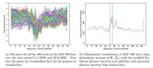
We apply the proposed method to a real data application from the US stock return data. The data set is available at https://www.finance.yahoo.com and can be obtained using the R package BatchGetSymbols for different time periods. The data we use here holds the daily closing prices of stocks from the S&P 500 index during the first year of COVID-19 pandemic between 1st January 2020 and 30th June 2020, which results in n = 125 time points and p = 496 stocks. This specific time period is chosen because based on the experts analysis reported in Statista Research Department (2022), the S&P 500 index showed much volatility and dropped by about 20% in early March 2020 entering into a bear market. While the drop was the steepest one-day fall since 1987, S&P 500 index began to recover at the start of April 2020. Stock markets fell in the wake of the COVID-19 pandemic, with investors fearing its spread could destroy economic growth. Figure 6(a) shows a rough display of the price changes for all the stocks over this time period, where all the stock prices are standardised for visualisation purpose. One can see the very steep drop around early March 2020, as explained. The drop seems to be happened for a majority of stocks with some different magnitudes, suggesting a non-sparse high dimensional change point problem here.

Figure 6(b) displays the dissimilarity visualisation of the S&P 500 data using the dissimilarity measure $d({\mathit{X}}_i,{\mathit{X}}_j)$ with both the modified Euclidean distance function and the univariate distance function, which show a similar trend. Note that the column sums of the two dissimilarity indices are drawn for those trading days in the first half of 2020. The figure suggests that the trading days 13th and 16th March 2020 show the largest total dissimilarity from all the other observations and are marked by vertical bars.

We first implement our distribution-free method, using our R package HDDchangepoint, to find significant change points in this high dimensional data set. Our method with the asymptotic test, using both distance functions, returns six change point locations, namely 51, 57, 66, 95, 106, 112. The method with the permutation test returns four change point locations, namely 51, 57, 66, 95. While the two tests produce four common change points, the permutation test is a bit conservative considering the dimension of data, which is in line with our numerical results. The asymptotic p-values for these four significant change points are $5.64\mathrm{e}-09,5.06\mathrm{e}-04,1.27\mathrm{e}-05$ and $2.50\mathrm{e}-07$, respectively. Also, the same four change points are obtained when we use 10 or 15 as the minimum segment length for the binary segmentation. We then apply the E-divisive method of Matteson and James (2014) with the minimum segment length being 15, which detects seven significant change points, namely 15, 37, 48, 68, 80, 95, 106. Also, the random projection method of Wang and Samworth (2018) finds nine change point locations, namely 18, 35, 44, 50, 65, 78, 99, 111, 124. The HDcpdetect method of Li et al. (2019) only finds two change point locations 48, 80. As in our numerical results, HDcpdetect tends to detect fewer change points when there are multiple change points (see Figures 5(a) and 5(b)), and the random projection method shows a lower accuracy in such high dimensional data with a small sample size (see Table 2). Considering our simulation results especially those in Table 2 for multiple change points, we believe our estimates of change point locations are more accurate, especially the detected locations 51 and 57 which coincide with the steep drop in the stock prices in early March 2020 due to the COVID-19 impact on the market. Some further results on our analysis of this data set is reported in Appendix C.

7 Concluding remarks

We have proposed a distance-based method for detecting single and multiple change points in non-sparse high dimensional data. The proposed approach is based on new dissimilarity measures and some proposed distance and difference distance matrices, which does not require normality or any other specific distribution for the observations. However, we note that our asymptotic tests require up to four finite moments of the distribution. Our method is especially useful for change point detection in HDLSS data when the sample size is very small compared to the dimension of data. This is an understudied problem in the literature of high dimensional change points. Our method can handle non-sparse high dimensional situations where changes may happen in many variables and with small significant magnitudes. We have introduced a novel test statistic to formally test the significance of estimated change points and established its asymptotic and permutation distributions to address both small and large sample size situations. We have shown that our proposed estimates of change point locations are consistent for the true unknown change points under some standard conditions and that our proposed tests are consistent asymptotically. Our simulation results showed that both asymptotic and permutation tests perform well compared to some of the recent methods for high dimensional change points. Our R package HDDchangepoint for implementation of the proposed method, including both the recursive binary segmentation and the wild binary segmentation as well as the real data application, can be obtained from “https://github.com/rezadrikvandi/HDDchangepoint“. The R package returns significant change point estimates and their corresponding p-values, and it can also be applied with any other dissimilarity measure specified by the user.

Disclosure statement

The authors report there are no competing interests to declare.

Table 1 Frequency and average number of the detected change points over 250 replications by each of the methods when there is one true change point, also including the case with no change point.

${\mathit{\mu }}_2$	n	p	Number of true change points	Method	Frequency of the detected change points	Average number of detected change points
					0	1
	45	500	0	Permutation	0.98	0.02	0.02
	45	500	0	Asymptotic	0.98	0.02	0.02
${\mathbf{0}}_p$	45	500	0	E-divisive	0.97	0.03	0.03
	45	500	0	Inspect	0.97	0.03	0.03
	45	500	0	HDcpdetect	0.98	0.02	0.02
	45	1000	0	Permutation	0.97	0.03	0.03
	45	1000	0	Asymptotic	0.96	0.04	0.04
${\mathbf{0}}_p$	45	1000	0	E-divisive	0.95	0.05	0.05
	45	1000	0	Inspect	0.94	0.06	0.06
	45	1000	0	HDcpdetect	0.96	0.04	0.04
	45	1500	0	Permutation	0.95	0.05	0.05
	45	1500	0	Asymptotic	0.95	0.05	0.05
${\mathbf{0}}_p$	45	1500	0	E-divisive	0.96	0.04	0.04
	45	1500	0	Inspect	0.94	0.06	0.06
	45	1500	0	HDcpdetect	0.96	0.04	0.04
	45	500	1	Permutation	0.80	0.20	0.20
	45	500	1	Asymptotic	0.73	0.27	0.27
$(0.1\times {\mathbf{1}}_{3p/4},0\times {\mathbf{1}}_{p/4})$	45	500	1	E-divisive	0.83	0.17	0.17
	45	500	1	Inspect	0.91	0.09	0.09
	45	500	1	HDcpdetect	0.87	0.13	0.13
	45	1000	1	Permutation	0.42	0.58	0.58
	45	1000	1	Asymptotic	0.33	0.67	0.67
$(0.1\times {\mathbf{1}}_{3p/4},0\times {\mathbf{1}}_{p/4})$	45	1000	1	E-divisive	0.67	0.33	0.33
	45	1000	1	Inspect	0.93	0.07	0.07
	45	1000	1	HDcpdetect	0.71	0.29	0.29
	45	1500	1	Permutation	0.16	0.84	0.84
	45	1500	1	Asymptotic	0.13	0.87	0.87
$(0.1\times {\mathbf{1}}_{3p/4},0\times {\mathbf{1}}_{p/4})$	45	1500	1	E-divisive	0.38	0.62	0.62
	45	1500	1	Inspect	0.93	0.07	0.07
	45	1500	1	HDcpdetect	0.49	0.51	0.51
	45	500	1	Permutation	0.12	0.88	0.88
	45	500	1	Asymptotic	0.10	0.90	0.90
$(0.2\times {\mathbf{1}}_{3p/4},0\times {\mathbf{1}}_{p/4})$	45	500	1	E-divisive	0.14	0.86	0.86
	45	500	1	Inspect	0.77	0.23	0.23
	45	500	1	HDcpdetect	0.15	0.85	0.85
	45	1000	1	Permutation	0.00	1.00	1.00
	45	1000	1	Asymptotic	0.00	1.00	1.00
$(0.2\times {\mathbf{1}}_{3p/4},0\times {\mathbf{1}}_{p/4})$	45	1000	1	E-divisive	0.03	0.97	0.97
	45	1000	1	Inspect	0.72	0.28	0.28
	45	1000	1	HDcpdetect	0.05	0.95	0.95
	45	1500	1	Permutation	0.00	1.00	1.00
	45	1500	1	Asymptotic	0.00	1.00	1.00
$(0.2\times {\mathbf{1}}_{3p/4},0\times {\mathbf{1}}_{p/4})$	45	1500	1	E-divisive	0.02	0.98	0.98
	45	1500	1	Inspect	0.63	0.37	0.37
	45	1500	1	HDcpdetect	0.02	0.98	0.98

Table 2 Frequency and average number of the correctly detected change points over 250 replications by each of the methods when there are three true change points, also including the case with no change points.

${\mathit{\mu }}_2$	n	p	Number of true change points	Method	Frequency of the detected change points	Average number of detected change points
					0	1	2	3
	90	500	0	Permutation	0.97	0.03	0.00	0.00	0.03
	90	500	0	Asymptotic	0.97	0.03	0.00	0.00	0.03
${\mathbf{0}}_p$	90	500	0	E-divisive	0.96	0.04	0.00	0.00	0.04
	90	500	0	Inspect	0.95	0.05	0.00	0.00	0.05
	90	500	0	HDcpdetect	0.96	0.04	0.00	0.00	0.04
	90	1000	0	Permutation	0.97	0.03	0.00	0.00	0.03
	90	1000	0	Asymptotic	0.96	0.04	0.00	0.00	0.04
${\mathbf{0}}_p$	90	1000	0	E-divisive	0.95	0.05	0.00	0.00	0.05
	90	1000	0	Inspect	0.96	0.04	0.00	0.00	0.04
	90	1000	0	HDcpdetect	0.95	0.05	0.00	0.00	0.05
	90	1500	0	Permutation	0.96	0.04	0.00	0.00	0.04
	90	1500	0	Asymptotic	0.96	0.04	0.00	0.00	0.04
${\mathbf{0}}_p$	90	1500	0	E-divisive	0.96	0.04	0.00	0.00	0.04
	90	1500	0	Inspect	0.94	0.06	0.00	0.00	0.06
	90	1500	0	HDcpdetect	0.94	0.06	0.00	0.00	0.06
	90	500	3	Permutation	0.32	0.46	0.20	0.02	0.92
	90	500	3	Asymptotic	0.24	0.48	0.26	0.02	1.06
$(0.1\times {\mathbf{1}}_{3p/4},0\times {\mathbf{1}}_{p/4})$	90	500	3	E-divisive	0.30	0.56	0.12	0.02	0.86
	90	500	3	Inspect	0.56	0.38	0.06	0.00	0.50
	90	500	3	HDcpdetect	0.32	0.62	0.06	0.00	0.74
	90	1000	3	Permutation	0.09	0.24	0.56	0.11	1.69
	90	1000	3	Asymptotic	0.06	0.27	0.50	0.17	1.77
$(0.1\times {\mathbf{1}}_{3p/4},0\times {\mathbf{1}}_{p/4})$	90	1000	3	E-divisive	0.07	0.60	0.23	0.10	1.36
	90	1000	3	Inspect	0.46	0.45	0.09	0.00	0.63
	90	1000	3	HDcpdetect	0.20	0.63	0.14	0.03	1.00
	90	1500	3	Permutation	0.00	0.05	0.19	0.76	2.71
	90	1500	3	Asymptotic	0.00	0.05	0.15	0.80	2.75
$(0.1\times {\mathbf{1}}_{3p/4},0\times {\mathbf{1}}_{p/4})$	90	1500	3	E-divisive	0.05	0.25	0.46	0.24	1.89
	90	1500	3	Inspect	0.22	0.58	0.19	0.01	0.99
	90	1500	3	HDcpdetect	0.08	0.44	0.38	0.10	1.50
	90	500	3	Permutation	0.00	0.02	0.18	0.80	2.78
	90	500	3	Asymptotic	0.00	0.02	0.16	0.82	2.80
$(0.2\times {\mathbf{1}}_{3p/4},0\times {\mathbf{1}}_{p/4})$	90	500	3	E-divisive	0.00	0.02	0.24	0.74	2.72
	90	500	3	Inspect	0.06	0.30	0.36	0.28	1.86
	90	500	3	HDcpdetect	0.01	0.45	0.14	0.40	1.93
	90	1000	3	Permutation	0.00	0.00	0.00	1.00	3.00
	90	1000	3	Asymptotic	0.00	0.00	0.00	1.00	3.00
$(0.2\times {\mathbf{1}}_{3p/4},0\times {\mathbf{1}}_{p/4})$	90	1000	3	E-divisive	0.00	0.00	0.14	0.86	2.86
	90	1000	3	Inspect	0.00	0.13	0.57	0.30	2.16
	90	1000	3	HDcpdetect	0.00	0.53	0.19	0.28	1.75
	90	1500	3	Permutation	0.00	0.00	0.00	1.00	3.00
	90	1500	3	Asymptotic	0.00	0.00	0.00	1.00	3.00
$(0.2\times {\mathbf{1}}_{3p/4},0\times {\mathbf{1}}_{p/4})$	90	1500	3	E-divisive	0.00	0.00	0.02	0.98	2.98
	90	1500	3	Inspect	0.00	0.08	0.35	0.57	2.49
	90	1500	3	HDcpdetect	0.00	0.85	0.04	0.11	1.26

Table 3 Frequency and average number of the detected change points over 250 replications by each of the methods when there is a true change in variance of observations.

$({\mathit{\mu }}_1,{\mathbf{\Sigma }}_1)$	$({\mathit{\mu }}_2,{\mathbf{\Sigma }}_2)$	n	p	Method	Frequency of the detected change points	Average number of detected change points
					0	1
$({\mathbf{0}}_p,0.5{\mathit{V}}_p)$	$({\mathbf{0}}_p,0.6{\mathit{V}}_p)$	45	500	Permutation	0.87	0.13	0.13
$({\mathbf{0}}_p,0.5{\mathit{V}}_p)$	$({\mathbf{0}}_p,0.6{\mathit{V}}_p)$	45	500	Asymptotic	0.85	0.15	0.15
$({\mathbf{0}}_p,0.5{\mathit{V}}_p)$	$({\mathbf{0}}_p,0.6{\mathit{V}}_p)$	45	500	E-divisive	0.98	0.02	0.02
$({\mathbf{0}}_p,0.5{\mathit{V}}_p)$	$({\mathbf{0}}_p,0.6{\mathit{V}}_p)$	45	500	Inspect	0.98	0.02	0.02
$({\mathbf{0}}_p,0.5{\mathit{V}}_p)$	$({\mathbf{0}}_p,0.6{\mathit{V}}_p)$	45	500	HDcpdetect	0.99	0.01	0.01
$({\mathbf{0}}_p,0.5{\mathit{V}}_p)$	$({\mathbf{0}}_p,0.6{\mathit{V}}_p)$	45	1000	Permutation	0.32	0.68	0.68
$({\mathbf{0}}_p,0.5{\mathit{V}}_p)$	$({\mathbf{0}}_p,0.6{\mathit{V}}_p)$	45	1000	Asymptotic	0.29	0.71	0.71
$({\mathbf{0}}_p,0.5{\mathit{V}}_p)$	$({\mathbf{0}}_p,0.6{\mathit{V}}_p)$	45	1000	E-divisive	0.96	0.04	0.04
$({\mathbf{0}}_p,0.5{\mathit{V}}_p)$	$({\mathbf{0}}_p,0.6{\mathit{V}}_p)$	45	1000	Inspect	0.96	0.04	0.04
$({\mathbf{0}}_p,0.5{\mathit{V}}_p)$	$({\mathbf{0}}_p,0.6{\mathit{V}}_p)$	45	1000	HDcpdetect	0.98	0.02	0.02
$({\mathbf{0}}_p,0.5{\mathit{V}}_p)$	$({\mathbf{0}}_p,0.6{\mathit{V}}_p)$	45	1500	Permutation	0.09	0.91	0.91
$({\mathbf{0}}_p,0.5{\mathit{V}}_p)$	$({\mathbf{0}}_p,0.6{\mathit{V}}_p)$	45	1500	Asymptotic	0.08	0.92	0.92
$({\mathbf{0}}_p,0.5{\mathit{V}}_p)$	$({\mathbf{0}}_p,0.6{\mathit{V}}_p)$	45	1500	E-divisive	0.96	0.04	0.04
$({\mathbf{0}}_p,0.5{\mathit{V}}_p)$	$({\mathbf{0}}_p,0.6{\mathit{V}}_p)$	45	1500	Inspect	0.97	0.03	0.03
$({\mathbf{0}}_p,0.5{\mathit{V}}_p)$	$({\mathbf{0}}_p,0.6{\mathit{V}}_p)$	45	1500	HDcpdetect	0.97	0.03	0.03
$({\mathbf{0}}_p,0.5{\mathit{V}}_p)$	$({\mathbf{0}}_p,0.7{\mathit{V}}_p)$	45	500	Permutation	0.09	0.91	0.91
$({\mathbf{0}}_p,0.5{\mathit{V}}_p)$	$({\mathbf{0}}_p,0.7{\mathit{V}}_p)$	45	500	Asymptotic	0.09	0.91	0.91
$({\mathbf{0}}_p,0.5{\mathit{V}}_p)$	$({\mathbf{0}}_p,0.7{\mathit{V}}_p)$	45	500	E-divisive	0.86	0.14	0.14
$({\mathbf{0}}_p,0.5{\mathit{V}}_p)$	$({\mathbf{0}}_p,0.7{\mathit{V}}_p)$	45	500	Inspect	0.97	0.03	0.03
$({\mathbf{0}}_p,0.5{\mathit{V}}_p)$	$({\mathbf{0}}_p,0.7{\mathit{V}}_p)$	45	500	HDcpdetect	0.98	0.02	0.02
$({\mathbf{0}}_p,0.5{\mathit{V}}_p)$	$({\mathbf{0}}_p,0.7{\mathit{V}}_p)$	45	1000	Permutation	0.00	1.00	1.00
$({\mathbf{0}}_p,0.5{\mathit{V}}_p)$	$({\mathbf{0}}_p,0.7{\mathit{V}}_p)$	45	1000	Asymptotic	0.00	1.00	1.00
$({\mathbf{0}}_p,0.5{\mathit{V}}_p)$	$({\mathbf{0}}_p,0.7{\mathit{V}}_p)$	45	1000	E-divisive	0.72	0.28	0.28
$({\mathbf{0}}_p,0.5{\mathit{V}}_p)$	$({\mathbf{0}}_p,0.7{\mathit{V}}_p)$	45	1000	Inspect	0.94	0.06	0.06
$({\mathbf{0}}_p,0.5{\mathit{V}}_p)$	$({\mathbf{0}}_p,0.7{\mathit{V}}_p)$	45	1000	HDcpdetect	0.97	0.03	0.03
$({\mathbf{0}}_p,0.5{\mathit{V}}_p)$	$({\mathbf{0}}_p,0.7{\mathit{V}}_p)$	45	1500	Permutation	0.00	1.00	1.00
$({\mathbf{0}}_p,0.5{\mathit{V}}_p)$	$({\mathbf{0}}_p,0.7{\mathit{V}}_p)$	45	1500	Asymptotic	0.00	1.00	1.00
$({\mathbf{0}}_p,0.5{\mathit{V}}_p)$	$({\mathbf{0}}_p,0.7{\mathit{V}}_p)$	45	1500	E-divisive	0.49	0.51	0.51
$({\mathbf{0}}_p,0.5{\mathit{V}}_p)$	$({\mathbf{0}}_p,0.7{\mathit{V}}_p)$	45	1500	Inspect	0.95	0.05	0.05
$({\mathbf{0}}_p,0.5{\mathit{V}}_p)$	$({\mathbf{0}}_p,0.7{\mathit{V}}_p)$	45	1500	HDcpdetect	0.96	0.04	0.04

Table 4 Frequency and average number of the detected change points over 250 replications by each of the methods when there is a change in distribution of observations while their mean and variance remain the same.

Two different distributions	n	p	Number of true change points	Method	Frequency of the detected change points	Average number of detected change points
					0	1
	45	500	1	Univariate	0.86	0.14	0.14
	45	500	1	L2 norm	0.84	0.16	0.16
	45	500	1	L1 norm	0.74	0.26	0.26
$N(0,5/3)$ & t(5)	45	500	1	E-divisive	0.55	0.45	0.45
	45	500	1	Inspect	0.99	0.01	0.01
	45	500	1	HDcpdetect	0.98	0.02	0.02
	45	1000	1	Univariate	0.83	0.17	0.17
	45	1000	1	L 2 norm	0.80	0.20	0.20
	45	1000	1	L 1 norm	0.69	0.31	0.31
$N(0,5/3)$ & t(5)	45	1000	1	E-divisive	0.51	0.49	0.49
	45	1000	1	Inspect	0.97	0.03	0.03
	45	1000	1	HDcpdetect	0.96	0.04	0.04
	45	1500	1	Univariate	0.80	0.20	0.20
	45	1500	1	L 2 norm	0.77	0.23	0.23
	45	1500	1	L 1 norm	0.66	0.34	0.34
$N(0,5/3)$ & t(5)	45	1500	1	E-divisive	0.50	0.50	0.50
	45	1500	1	Inspect	0.94	0.06	0.06
	45	1500	1	HDcpdetect	0.94	0.06	0.06
	45	500	1	Univariate	0.99	0.01	0.01
	45	500	1	L2 norm	0.98	0.02	0.02
	45	500	1	L1 norm	0.58	0.42	0.42
N(1, 1) & $\hspace{0.17em}\mathrm{Exp}\hspace{0.17em}(1)$	45	500	1	E-divisive	0.99	0.01	0.01
	45	500	1	Inspect	0.96	0.04	0.04
	45	500	1	HDcpdetect	0.99	0.01	0.01
	45	1000	1	Univariate	0.98	0.02	0.02
	45	1000	1	L2 norm	0.95	0.05	0.05
	45	1000	1	L1 norm	0.29	0.71	0.71
N(1, 1) & $\hspace{0.17em}\mathrm{Exp}\hspace{0.17em}(1)$	45	1000	1	E-divisive	0.98	0.02	0.02
	45	1000	1	Inspect	0.94	0.06	0.06
	45	1000	1	HDcpdetect	0.98	0.02	0.02
	45	1500	1	Univariate	0.96	0.04	0.04
	45	1500	1	L2 norm	0.90	0.10	0.10
	45	1500	1	L1 norm	0.09	0.91	0.91
N(1, 1) & $\hspace{0.17em}\mathrm{Exp}\hspace{0.17em}(1)$	45	1500	1	E-divisive	0.92	0.08	0.08
	45	1500	1	Inspect	0.93	0.07	0.07
	45	1500	1	HDcpdetect	0.97	0.03	0.03

Figure 1 Illustrative example with one change point: plots for all elements of the distance matrix D obtained using the dissimilarity measure $d({\mathit{X}}_i,{\mathit{X}}_j)$ in (3) with both the univariate and multivariate distance functions, as well as for all column sums of the difference distance matrix Δ.

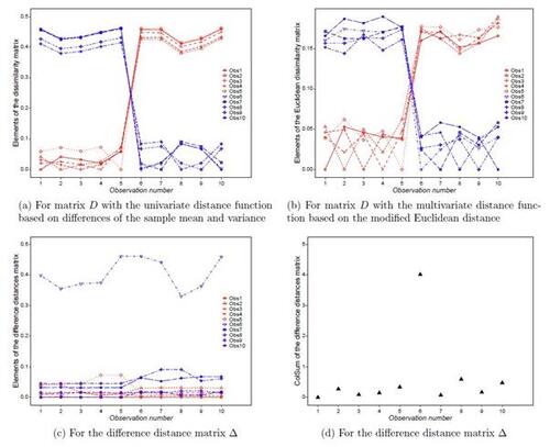
Figure 2 The sets ${\nabla }_{\widehat{\tau }}^{-}$ and ${\nabla }_{\widehat{\tau }}^{+}$ with the estimated change point location $\widehat{\tau }$.

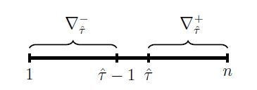
Figure 3 Illustrative example with two change points: plots for all elements of the distance matrix D obtained using the dissimilarity measure $d({\mathit{X}}_i,{\mathit{X}}_j)$ in (3) with both the univariate and multivariate distance functions, as well as for all column sums of the difference distance matrix Δ.

Figure 4 The estimate of change point from each of the methods over 250 replications with a true single change point at location $3n/5+1=28$ when n = 45.

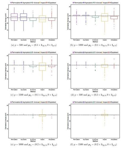
Figure 5 Average number of the total change points detected (correct or incorrect detection) over 250 replications by each of the methods for multiple change point detection.

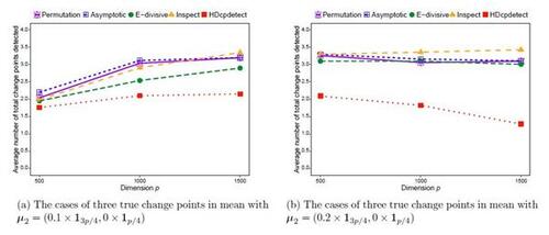
Figure 6 Change point plots for the S&P 500 data over the time period 1/1/2020 and 30/6/2020 during the COVID-19 pandemic. In plot (b) the two trading days 13th and 16th March 2020 show the largest total dissimilarity from all the other days and are marked by vertical bars (in green).