Fish early life stage toxicity prediction from acute daphnid toxicity and quantum chemistry

ABSTRACT

One step towards reduced animal testing is the use of in silico screening methods to predict toxicity of chemicals, which requires high-quality data to develop models that are reliable and clearly interpretable. We compiled a large data set of fish early life stage no observed effect concentration endpoints (FELS NOEC) based on published data sources and internal studies, containing data for 338 molecules. Furthermore, we developed a new quantitative structure-activity-activity relationship (QSAAR) model to inform estimation of this endpoint using a combination of dimensionality reduction, regularization, and domain knowledge. In particular, we made use of a sparse partial least squares algorithm (sPLS) to select relevant variables from a huge number of molecular descriptors ranging from topological to quantum chemical properties. The final QSAAR model is of low complexity, consisting of 2 latent variables based on 8 molecular descriptors and experimental Daphnia magna acute data (EC50, 48 h). We provide a mechanistic interpretation of each model parameter. The model performs well, with a coefficient of determination r² of 0.723 on the training set (cross-validated q² = 0.686) and comparable predictivity on a test data set of chemically related molecules with experimental Daphnia magna data (r²_test = 0.687, RMSE = 0.793 log units).

KEYWORDS:

• Fish early life stage (FELS) toxicity
• quantitative structure-activity-activity relationship (QSAAR)
• sparse partial least squares (sPLS)
• variable selection
• acute Daphnia magna toxicity

Introduction

The fish early life stage test (FELS) according to OECD guideline 210 [1] is the primary test system required for measuring chronic toxicity of regulated chemicals (pesticides, industrial chemicals, pharmaceuticals, food/feed additives, and cosmetics) to fish. It is used to screen and prioritize hundreds to thousands of chemicals regulated under Registration, Evaluation, Authorization and Restriction of Chemicals (REACH), Toxic Substances Control Act (TSCA), and other national or international chemical management programmes. Consequently, many publications on this topic can be found in the literature. To mention only a few, reviews on the induced toxicity of fungicides to fish [2], the effect of herbicides [3], insecticides [4], and pharmaceuticals [5] have been published. A survey of the literature describing the effects of pesticides to fish in general is given in ref [6].

In silico methods could help estimating the toxicity in cases where no experimental data are available and to reduce the number of studies for less toxic compounds which do not require high precision for risk assessment or risk management decisions. This is in line with the strategy of the European Commission to replace, reduce and refine the use of fish in aquatic toxicity and bioaccumulation testing, documented by the European Union Reference Laboratory for Alternatives to Animal Testing (EURL ECVAM) [7]. One means to avoid chronic toxicity studies of chemicals consists in extrapolating from their acute toxicity to their chronic toxicity values in fish. Several approaches using acute-to-chronic ratios (ACRs) are available [8,9]. Most commonly the ACR is defined as the ratio of acute fish 96 h toxicity (LC50 or EC50) to the NOEC (no observed effect concentration) or the MATC (maximum acceptable toxicant concentration), the latter being the geometric mean of chronic NOEC and LOEC (lowest observed effect concentration) of the same species. For a critical review by Scholz et al. see ref [10]. These authors found that the ACRs may differ by two orders of magnitude depending on the modes of action of the chemicals. Hence, mode of action-specific models would be required to predict chronic fish toxicity from acute fish toxicity. However, the relevant mode of action causing an effect in the chronic study might be different compared to the acute study.

Quantitative structure–activity relationships (QSARs) are alternative in silico approaches to estimate toxicity, describing molecules by their molecular properties. Example QSAR models exist for chronic fish toxicity in form of the NOEC, based on the octanol-water distribution coefficient (log Kow) as the only descriptor [11,12]. These models have been criticized for not complying with the OECD and REACH criteria because of design errors in the setup of the QSARs [13,14]. As an example, these authors found a replication of compounds in the training set, resulting in misleading statistics for the robustness and predictivity of the models, inadequate data from sub-chronic tests as well as acids and product mixtures. For that reason, they developed log Kow based models for sublethal NOECs for non-polar narcotics [14] or for both polar and non-polar narcotics using log Kow and pKa as descriptors [13]. However, these are based on a rather limited number of compounds and thus do not cover a large chemical space.

Recently, Furuhama et al. [15] published QSAAR models (Quantitative Structure-Activity-Activity Relationship) for the prediction of the fish NOEC endpoint based on 77 molecules and acute toxicity towards daphnids (EC50, 48 h). The advantage of using experimental daphnid data as predictor variable in a model lies within its ability to account for very specific modes of action that could otherwise not be accounted for with molecular features, especially when only a few hundreds of data points are available. Such activity-activity models can be understood as a way to focus the prediction on the difference between the two species, which is a much easier task than prediction of chronic fish toxicity without such prior knowledge. Of course, this comes at the price of having experimental data available. However, the acute daphnid study is much less complex and more readily available than a chronic fish study. And most importantly, it is not a vertebrate study, which should be reduced to a minimum for animal welfare reasons. Using the acute daphnid data, Furuhama et al. were able to surpass the predictivity of purely structure-based QSAR models. However, the data set used for model training is still relatively small. Although many crop protection active ingredients are present in their data set, we noticed that FELS data are available for additional chemical classes, which inspired us to update our existing model (unpublished and superseded by this work) based on an extended data set.

In this study, we developed new QSAAR models for the prediction of fish NOEC values with the aim to improve the accuracy of the predictions compared to previous models and to extend the model’s applicability domain (AD) towards more crop protection chemical classes. It should be mentioned that the NOEC has been criticized for being misleading and statistically unfounded and that EC10 values (10^th percentile of the concentration–response curve) should be preferred [16,17]. On the other hand, robust calculation of an EC10 is often not feasible as the number of effect concentrations with different effect size is low, leading to high uncertainty in the fit of a dose response curve. In FELS studies multiple life stages and endpoints with different effect sizes are investigated, e.g. hatch, larval survival, time to swim up, length and weight. At the same time, test concentrations and group sizes should not be unnecessarily increased due to animal welfare reasons. Therefore, it is nearly impossible to design a FELS test in a way that all endpoints result in dose response curves of sufficient quality to allow a robust EC10 calculation. Thus, a FELS study will most frequently result only for some endpoints in an EC10 while the other endpoints will still result in a NOEC. Moreover, most historic FELS studies aimed for the derivation of a NOEC. Therefore, the data basis of NOEC values is larger compared to EC10 values, increasing the power of statistical modelling methods like QSAR. The maximum factor of 3.2 between test concentrations [1] assures that the NOEC/LOEC comparison stays within a narrow concentration range. The minimum detectable difference associated with the NOEC is frequently around 10%. For European risk assessments, both EC10 and NOEC are used [18,19]. In our current study, we focused on NOEC values because it allowed model development on a large and broad compound basis, which is a prerequisite for structure-based models.

In total, we compiled NOEC data for 338 chemicals, based on published and internal studies. As a modelling technique, we primarily used PLS (partial least squares) and its regularized variant sPLS, which is suitable for variable selection. PLS is a dimensionality reduction technique, which optimizes the covariance between dependent (pNOEC) and independent (descriptors) latent structures. In contrast to conventional linear or multilinear regression (MLR) approaches found in many ecotoxicological QSARs, PLS is suitable even for ill-posed problems with many more variables than observations (p > n), and multi-collinearities among the variables [20,21]. Moreover, it is less prone to overfitting, i.e. the gap in predictivity on the training set and an external test set is usually small [20]. The regularized sPLS variant serves as variable selection by enforcing a penalty on the descriptor loadings, shrinking many of them to zero. This improves predictivity and interpretability. It performs well on small and difficult data sets compared to more complex and non-linear machine learning algorithms [22].

In the subsequent sections, we outline the model development, including construction of the data set and the choice of the optimum model dimensions, analyse the final PLS model mechanistically, and compare it to existing models from the literature.

Materials and methods

Experimental data

The fish early life stage study (FELS) aims to determine the chronic toxicity of chemical substances to the different life stages of fish species. The following effects are examined in comparison to a control group at multiple concentrations: hatching success, time to swim up, larval survival, morphology, behaviour, and growth in terms of length, wet weight, and dry weight. We collected NOEC endpoints from FELS studies, which is the highest test concentration at which no statistically significant adverse effects were observed. One limitation we saw in previous attempts to model FELS studies was the low number of compounds with available data. We therefore combined multiple data sources, which has the additional advantages that bias resulting from the scope of a data source is reduced (e.g. focus on a certain chemical space), and errors can be detected when values for the same compound do not match between the sources. Prerequisites for the combination are careful curation and the same nature of the underlying data across sources, i.e. guideline FELS studies as described below. We collected NOEC endpoints for multiple fish species from the sources below, focussing on the most data-rich species per source. Further steps to increase consistency and representativity of our data set are described thereafter.

1. Internal studies from Bayer AG, Crop Science Division: This set contains more than 100 FELS studies from the crop protection chemical space. The studies were selected carefully according to several criteria: the studies must be according to accepted international guidelines valid at the time of study conduct (FIFRA guideline 72–4, OCSPP guideline 850.1400, OECD TG 210) the pure compound was tested, and the study produces a valid and reliable NOEC value according to the criteria used in the EU regulatory process. The set contains data for 92 compounds, of which 73 values are bounded NOEC values (i.e. ‘ = ’) and 19 studies report only lower limits (i.e. ‘≥’) because even at the highest test concentration no effect was observed. This set represents the core of our overall dataset, with highest confidence in data quality for QSAR modelling.

2. EFSA OpenFoodTox database [23], version 2, 2018: Search criteria for this set were bounded NOEC values for Pimephales promelas (fathead minnow) and Oncorhynchus mykiss (rainbow trout) and a realistic study duration for the two species in order to ensure that the test is indeed a suitable FELS test. This set contains FELS endpoints for 122 substances.

3. OECD QSAR Toolbox [24], version 4.3, 2019: We queried all relevant databases within the Toolbox, including US-EPA ECOTOX, Aquatic ECETOC, Aquatic Japan MoE, and Aquatic OASIS, with the following query parameters: test type = ‘Early Life Stage’ or organism characteristics = ‘ErlyLf’; species: Pimephales promelas (fathead minnow), Oncorhynchus mykiss (rainbow trout), Cyprinodon variegatus (sheepshead minnow), Danio rerio (zebrafish), with a study duration typical for FELS tests (20–100 days, depending on the species). We kept only bounded NOEC endpoints (‘ = ’) with an effect type typical for FELS tests. In total, 206 endpoints for 183 compounds were found.

4. Furuhama et al. [15]: This publication contains a set of FELS endpoints for 124 compounds for Pimephales promelas (fathead minnow) and Oryzias latipes (medaka). The data set was carefully curated by the authors with the aim to develop QSAR models.

In total, we compiled experimental NOEC values for 338 compounds, representing the species Pimephales promelas (fathead minnow, 179 compounds), Oncorhynchus mykiss (rainbow trout, 113 compounds), Oryzias latipes (medaka, 41 compounds), Cyprinodon variegatus (sheepshead minnow, 31 compounds), and Danio rerio (zebrafish, 7 compounds).

In addition to the FELS data, we collected experimental data for Daphnia magna EC50 endpoints, which considers immobilization and mortality equally. The OECD QSAR Toolbox and EFSA OFT database were queried (species = Daphnia magna, duration = 48 h, bounded (‘ = ’) EC50/LC50 values). In total, we gathered Daphnia EC50 values for 259 out of the 338 compounds in our data set.

Data pre-processing. All experimental NOEC concentrations were converted to negative logarithmic molar quantities (pNOEC), where

(1) $\mathrm{p}\mathrm{N}\mathrm{O}\mathrm{E}\mathrm{C}=-\mathrm{l}\mathrm{o}\mathrm{g}\mathrm{N}\mathrm{O}\mathrm{E}\mathrm{C}\left(mmol/L\right)$(1)

is the negative decimal logarithm of the NOEC value for fish in an early life stage test given in millimolar units (mmol/L). For nearly 40% of the compounds more than one study was available. In most cases, the endpoints from these studies were identical or similar, but for multiple compounds, we found discrepancies in NOEC values in the same species, which we investigated and curated individually: we removed compounds with different (>1 log unit) activities of stereoisomers, corrected obvious errors (e.g. mg/L instead of µg/L), and preferred newer studies according to a new study design over older studies. Eight compounds with large unresolved discrepancies (standard deviation > 1 log unit) were removed from the data set (listed in Supporting Information). For the remaining compounds, there was sufficiently good agreement between the data sources. To account for the careful curation of our internal data as well as regulatory relevance, we selected the first value for each compound/species combination in the following order: internal studies > EFSA OpenFoodTox > scientific literature > QSAR toolbox. As the values are identical or similar, this order has only a minor impact on our dataset.

In a second step, we looked at differences between species. For 30 compounds we had data for more than one species available. Most of them on Pimephales promelas (fathead minnow), Oncorhynchus mykiss (rainbow trout), and Cyprinodon variegatus (sheepshead minnow), between which we observed approximately 1:1 relationships (see section Inter-species correlation in the Supporting Information). Data on the other species was too sparse. Good correlations have also been reported by others for acute fish toxicity for fathead minnow and medaka [15,25]. Based on the observed relationships and most of the differences being below 1 log unit, we estimate the impact of inter-species differences on the final data set to be low. Therefore, we averaged the pNOEC values over all species per compound and decided to build a model on the complete dataset as opposed to multiple species-specific models on much smaller datasets.

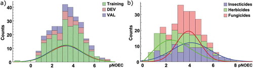
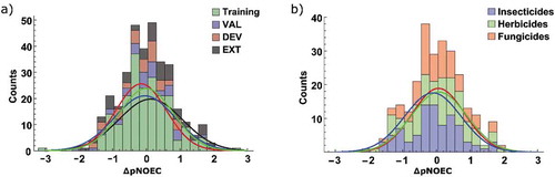
The pNOEC values of our data set span a range of almost 9 log units and are approximately normally distributed (Figure 1(a)). Focussing on the pesticides in the data set and classifying them according to their main indication reveals that insecticides tend to have higher pNOECs while herbicides have their maximum at lower values and fungicides concentrate at the centre of the distribution (Figure 1(b)). This is not surprising as important herbicidal targets like the Photosystem II are not present in fish, while many insecticides act on conserved targets in vertebrates and invertebrates (e.g. nervous system).

Figure 1. Distribution of pNOEC values as counts and normalized distribution functions a) for the chemicals in the training, DEV, and VAL set as defined in the Model development section, and b) according to their main pesticidal indication

Molecular structures and descriptors

Molecular structures were standardized with RDKit [26] to canonical SMILES, including neutralization and removal of ambiguous stereo information. Inorganic compounds and compounds containing heavy metals like Pb, Hg, Sn, or Cu were filtered out because of their special and unrepresentative properties. Salts and solvent molecules were stripped off. Duplicate compounds were merged neglecting stereo information and taking the mean pNOEC. We obtained 3D molecular structures with Schrödinger’s LigPrep [27] tool, including enumeration of undefined chiral centres, tautomers, and protonation to the prevailing charge state at pH 7. The structures were pre-optimized with the OPLS force field with solvent water. The lowest energy structure was further optimized with density functional theory (Turbomole 7.0.1 [28], BP86 functional, def2-TZVP basis set) and the COSMO-RS solvent model [29,30] accounting for solvent effects (water).

We used multiple software packages to calculate molecular descriptors from the pre-processed SMILES codes: CDK (v2.3) [31]; the RDKit KNIME nodes (version 3.8.0.v201906261723) [26,32] for molecular descriptors as well as Morgan fingerprints (1024 bits, radius 2) and MACCS keys; Sybyl [33] for Unity fingerprints. Additional descriptors were calculated based on neutral 3D molecular structures with Dragon 7.0 [34], PaDEL 2.21 [35], and with quantum-chemical methods (Turbomole 7.0.1 [28] and COSMOtherm X16 [30]) based on the prevailing charge state at pH 7 and at the minimum energy geometry at the BP86/def2-TZVP/COSMO-RS(water) level. Note that the support for the Dragon software has been discontinued in the meantime, but we confirmed that its successor software alvaDesc [36] is able to reproduce the calculated descriptors. In general, software versions and structure pre-processing steps must be checked with scrutiny to ensure consistent descriptor values.

We pre-processed the descriptor data table in the following way: We removed descriptors which had more than 3% missing values, more than 98% constant values, or were correlated to already selected descriptors with a correlation coefficient >0.95. Numeric outlier values were capped, i.e. values deviating from the first (Q₁) or third quartile (Q₃) by more than 1.5 times the interquartile range (Q₃ – Q₁) were replaced by the closest permitted value. Descriptors were mean-centred and normalized to standard deviation (Z-score normalization). Remaining missing values were filled with the mean.

Model development

Given the limited size of the data set, our strategy for selecting the training and test sets was mainly focused on building a broadly applicable predictive model, which requires high diversity in the selected sets. For the training set, we selected 60% of the compounds by Tanimoto dissimilarity based on the Unity fingerprints, using the MaxMin algorithm [37] as implemented in RDKit in KNIME. It incrementally picks compounds with the least similarity to the most similar compound from the already selected set. The Tanimoto similarity T is defined as

(2) $\mathrm{T}\left(\mathrm{a},\mathrm{b}\right)=\frac{{\mathrm{N}}_{\mathrm{a}\mathrm{b}}}{{\mathrm{N}}_{\mathrm{a}}+{\mathrm{N}}_{\mathrm{b}}-{\mathrm{N}}_{\mathrm{a}\mathrm{b}}}$(2)

where N_a and N_b are the numbers of 1-bits present in the fingerprint bitstrings of compounds a and b and N_ab is the number of 1-bits occurring in both fingerprints. From the remaining compounds, we selected 80% with the same procedure and split them in equal parts into development (DEV) and validation (VAL) set. This selection procedure constructs broad and diverse sets and reduces the bias from overly represented chemical classes in the data set. In total, 206 compounds were selected for the training set, and 38 and 39 for the DEV and VAL sets, respectively. The 55 extra compounds which belong to none of the previous sets are denoted as EXT set and were not used. The purpose of the DEV set was to monitor predictivity during model development and to make a few high-level decisions, e.g. to exclude all fingerprint descriptors. It was not used in fitting or optimization routines. The VAL set was completely held out during the model development phase and was only used as external test set to estimate the predictivity of the final models.

As modelling algorithm, we used Partial Least Squares (PLS [38], implemented in SIMCA [39]) and sparse Partial Least Squares (sPLS [40], implemented in the mixOmics R package [41]) on the pre-processed descriptor values as X-block and the pNOEC values as a single Y variable. The sPLS implementation in the mixOmics [41] package allows the user to select the number of latent variables (LV) and the number of descriptors per LV. The algorithm incrementally constructs latent variables, enforcing a regularization penalty such that only a selected number of descriptors have loading values different from zero. The selected descriptors can be different for each LV.

We trained the models exclusively on the training set. For evaluating the goodness of fit and predictive performance of the models, we calculated the following statistics on the training, DEV, and VAL sets as specified: the coefficient of determination r² for pNOEC, its cross-validated counterpart q² on the left-out batches of the training set from 5-fold cross-validation, and the root mean square error (RMSE).

The applicability domain (AD) of the PLS models was determined with default settings in SIMCA. Here, AD membership is determined by the variable PModXPS, the probability that the observation fits the model. It is computed from the distance of the prediction to the model plane in descriptor-space. An AD membership probability PModXPS > 0.05 indicates that a prediction is meaningful. However, a high membership probability is not related to a low error of an actual prediction.

Results and discussion

Selection of descriptor packages

From the plethora of software packages for calculating molecular descriptors, we selected frequently used ones and built sPLS [40] models for each descriptor package individually, to estimate its suitability for the pNOEC_FELS prediction task. The cross-validated results for two representative model complexities are summarized in Table 1. Please note that the categorization of descriptors into software packages is somewhat arbitrary and lacking physical reasoning. However, it can support the pre-selection decision based on effort, computation time, or licence costs. In general, the goodness of fit (in terms of r²) increases with a higher model complexity, especially for the larger packages, while the cross-validated q² does not increase, which indicates overfitting. A small number of variables seems sufficient to capture the overall trends in pNOEC.

Table 1. Comparison of descriptor packages and their performance in training (r²) and cross-validation (q²) for a less complex model (3 latent variables (LVs) with 5 descriptors each) and a more complex model (5 LVs without regularization)

Software package	Number of descriptors	Number of descriptors without constant/correlated/missing	3 LVs à 5 descriptors		5 LVs, whole package
			r^2	q^2	r^2	q^2
CDK	223	132	0.512	0.401	0.610	0.400
RDKit	76	63	0.509	0.399	0.613	0.413
PaDEL	1875	891	0.581	0.421	0.778	0.415
Dragon	5270	1714	0.573	0.372	0.749	0.447
QM	40	19	0.511	0.450	0.535	0.452
MACCS	167	126	0.340	0.148	0.447	0.101
Morgan	1024	390	0.192	0.039	0.230	0.054
Unity	992	843	0.296	0.082	0.584	0.058
ALL	9667	4178	0.642	0.391	0.801	0.455

The first four entries in Table 1 are frequently used molecular descriptor packages: CDK, RDKit, PaDEL, Dragon. These contain a wide mix of computed molecular properties (e.g. log P), constitutional, topological, geometric, and various other 2D and 3D descriptors, including some quantum-chemical properties calculated with fast semi-empirical methods. The two big sets from Dragon and PaDEL do not provide better predictivity (q²) than the smaller sets from CDK and RDKit but do provide a better fit to the training data (r² of up to 0.78 compared to 0.61). Notably, the quantum chemical (QM) descriptors as the smallest set achieved the best predictive power with a q² of 0.45. We therefore decided to keep these descriptors in our further analysis, although they are by far the most expensive descriptors in terms of manual labour and computation time. This set contains frontier orbital energies (HOMO, LUMO), dipole moment, polarizability, and surface properties from the COSMO-RS solvation model. The fingerprints (MACCS, Morgan, Unity) are less suitable for this particular regression task. We thus decided to drop the fingerprints for our further analysis. Fingerprints are binary vectors encoding the presence or absence of substructure entities.

Recently, Furuhama et al. [15] reported increased predictivity of FELS QSAR models when experimental daphnid toxicity (pEC50) was included as a descriptor. We therefore included this biological descriptor in our further model development and observed consistently high importance of this variable in the models we built (see e.g. Table S3 in the SI). Additionally, from the whole set of descriptors, it is the variable with the highest correlation to pNOEC (Pearson’s correlation coefficient of 0.67). Note that for around 25% of the data set the daphnid pEC50 values were missing and were imputed by assuming the mean value. We expect potential improvement of our models upon filling these missing values. Removing these compounds from the training set, however, did not result in improved or qualitatively different models. On the flipside, their removal would reduce the diversity in chemical space and hence the model’s applicability domain.

Overall, Table 1 indicates that the complexity of the models can be drastically decreased while maintaining most of the predictive power. This is desirable both to avoid overfitting on spurious correlations and to increase the interpretability of the models.

Model development

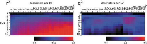
Having identified a suitable set of descriptors, we used the sPLS technique to further explore the ideal model complexity, i.e. a reasonable number of latent variables (LV) and descriptors per LV. Figure 2 shows the model’s coefficient of determination r² and its cross-validated counterpart q² over a broad range of model complexity. r² increases with the number of LVs and descriptors, reaching 0.95 for 10 LVs and 1000 descriptors. This is expected because the increased number of variables leads to a more flexible and better fit to the experimental data. However, one must be aware that this leads to overfitting to the data, which is no longer meaningful and is not indicative for the model’s predictivity on new compounds.

Figure 2. Goodness of fit (r²) and cross-validated q² of sPLS models with increasing numbers of latent variables (LV) and descriptors per LV from the packages CDK, RDKit, PaDEL, Dragon, QM, and pEC50 daphnid

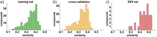
To evaluate the predictive power on the set of training compounds, we carried out a 5-fold cross-validation, fitting the model to only 80% of the training data and predicting the remaining 20%. Due to our focus on diversity during selection of compounds for the training set, this means that the predicted held-out compounds are relatively dissimilar to the remaining compounds of the training set (Figure 3). Therefore, the model bridges larger distances in chemical space, which is more difficult than predicting more similar compounds. Thus, the cross-validated coefficient of determination (q²) is relatively low, but more informative than a q² obtained from leave-one-out procedures.

Figure 3. Average similarity to the 5 most similar compounds from the training set, based on Tanimoto distance of Unity fingerprints. For the training (left) and DEV (right) sets, all compounds from the training set were considered, while for the cross-validation (middle) only compounds from the other CV-batches were considered

From Figure 2 we conclude that model predictivity in terms of q² is highest for 3 to 6 latent variables. The number of selected descriptors is less important, with a local maximum between 5 and 9 descriptors per LV, but also relatively high q² for up to 400 descriptors. The latter maximum has two main reasons: First, PLS and sPLS are well suited for problems with many noise variables in the data set [21]. We tested this hypothesis with a synthetic dataset and found a similar pattern with relatively high q² values for increased numbers of noise variables (see Figure S3). Second, many descriptors in our dataset are related to lipophilicity (log P), i.e. around 300 have correlation coefficients with ALOGP above 0.5 (Figure S4). In combination with log P being one of the most important descriptors for the pNOEC task, one of the prominent trends across all descriptors (which PLS extracts as latent variables) is lipophilicity, which remains predictive even for higher numbers of descriptors. However, it is of course desirable to find a model that uses fewer descriptors to describe lipophilicity, that can be interpreted more easily.

Our aim for further model development was to improve the global predictivity for the whole relevant chemical space (high q²) by reducing the model complexity with the help of mechanistic understanding and domain knowledge of human experts. The major steps of our model development process along with performance statistics of the associated models M1 to M6 are summarized in Table 2. As already discussed, using all descriptors from the most relevant packages leads to unsatisfying predictivity both during cross-validation and testing on the DEV set (model M1, Table 2). Reducing the number of descriptors by means of regularization (sPLS) can improve the predictivity. The two maxima of the q² grid scan from Figure 2 improve q² from 0.46 to 0.55 and 0.53, respectively (models M2 and M3, Table 2). From these two models, the less complex model M3 performs better on the DEV set, indicating that it is less overfitting to the training data. Note that r²_dev is higher than q² in some cases, which is again due to lower similarity of the compounds during cross-validation (see Figure 3). However, we included the statistics of models M1 to M4 only as representative landmarks in the model development process and do not recommend them for prediction purposes. Model M3 might be regarded as the best model coming from the automated approach, i.e. without manual refinement based on expert knowledge.

Table 2. Model performance summary along the major development steps, starting from all descriptors (CDK, RDKit, PaDEL, Dragon, QM and pEC50 daphnid) and gradually refining the model while reducing its complexity

Model	#LV/#descr.	r^2	q^2	r^2dev	RMSE (training)	RMSE (cross-val.)	RMSE (DEV)
M1, PLS with all descriptors	2/2225	0.554	0.463	0.452	0.961	1.060	1.025
M2, sPLS with max. q^2 (3x100)	3/294	0.693	0.546	0.493	0.798	0.986	0.986
M3, sPLS local max. q^2 (4x7)	4/27	0.698	0.534	0.647	0.791	1.048	0.822
M4, sPLS pre-selection (10x5)	10/50	0.815	0.415	0.632	0.618	1.100	0.840
M5, manual refinement	3/18	0.757	0.694	0.700	0.709	0.775	0.758
M6, manual refinement	2/9	0.723	0.686	0.729	0.757	0.808	0.720

#LV/#descr: number of latent variables (LVs) and descriptors, e.g. the sPLS model with 3 LVs and 100 descriptors each (‘3x100ʹ) has nearly 300 descriptor variables in total. Descriptor variables may be selected for multiple latent variables.

r², q², RMSE as explained in Materials and methods section.

We then started our manual refinement from a pre-selection of 50 descriptors, coming from an sPLS model with 10 LVs with 5 descriptors each (‘10x5ʹ model M4). This selection contains the important descriptors of the best sPLS model with 4 LVs à 7 descriptors (‘4x7ʹ model M3) and provides enough options for refinement without including too many descriptors for a manual selection process. Other sPLS models with a similar total number of descriptors could have equally been chosen as starting point. Subsequently, we fine-tuned a PLS model with the commercial software SIMCA [39] by manually removing or replacing single descriptors from this set. In addition to optimal predictivity as primary goal, the guiding principles were reduced model complexity, mechanistically interpretable descriptors, and preference for descriptors which are freely available and fast to compute, if possible. We also removed descriptors, whose loadings were not significantly different from zero (cross-validated), or relevant only for a few molecules. This procedure has not been automated and is mainly based on expert judgements and discussions in multiple rounds of optimization. Frequently, the optimization criteria were conflicting, and trade-offs had to be balanced. However, we found it invaluable to include expert knowledge as final refinement step. By applying our principles, we identified two PLS models with 3 LVs with 18 total descriptors (model M5) and 2 LVs with 9 total descriptors (model M6), respectively. These models outperform the automated selection approach both in cross-validation and on the DEV set, which supports our hypothesis that domain knowledge and a rigorous focus on reducing model complexity is favourable. The r²_dev values are above 0.7 and the root mean square errors are 0.758 and 0.720 for model M5 and M6, respectively. From these performance metrics models, M5 and M6 are nearly indistinguishable. However, we prefer model M6 over M5 due to its lower complexity.

Analysis of model M6 and mechanistic interpretation

The final model M6 is composed of two latent variables consisting of 9 descriptors, which are shown in the loadings plot in Figure 4 and described in Table 3. Descriptors near the blue pNOEC point are positively related with pNOEC while descriptors with negative loadings are inversely related to pNOEC. Equation 3(3) $\mathrm{p}\mathrm{N}\mathrm{O}\mathrm{E}\mathrm{C}=-log\left(NOEC\left[mM\right]\right)=a+\sum c_i{d}_i$(3) states the PLS model equation in a general multiple linear regression (MLR)-like format. The corresponding coefficients c_i for descriptor values d_i of the pre-processed descriptors for use with model M6 are given in Table 3.

(3) $\mathrm{p}\mathrm{N}\mathrm{O}\mathrm{E}\mathrm{C}=-log\left(NOEC\left[mM\right]\right)=a+\sum c_i{d}_i$(3)

Table 3. Model coefficients (c_i) and descriptors for use with equation 3(3) $\mathrm{p}\mathrm{N}\mathrm{O}\mathrm{E}\mathrm{C}=-log\left(NOEC\left[mM\right]\right)=a+\sum c_i{d}_i$(3) and model M6 (for more detailed descriptions see Table S2 in the Supporting Information)

ci (norm.)	Descriptors i	Description	Class
– 0.236367	hBondacceptors_CDK2	Number of hydrogen bond acceptor sites	1D
0.193715	HATS1p_Dragon	Leverage-weighted autocorrelation of lag 1/weighted by polarizability (GETAWAY 3D-autocorrelation)	3D
0.490086	ALOGP_Dragon	Ghose-Crippen octanol-water partition coeff. (logP)	2D
0.236732	DLS_03_Dragon	Modified drug-like score from Walters et al. (6 rules)	1D
0.213228	PolarisabilityAnisotropy_QM	Anisotropy of the static polarizability tensor	3D
– 0.333269	COSMORS_Hacc_QM	COSMO-RS hydrogen bond acceptor moment	3D
0.266294	slogp_VSA3_RDKit	Van der Waals surface area with logP from −0.20 to 0.00	2D
0.328670	smr_VSA4_RDKit	Van der Waals surface area with molecular refractivity from 2.24 to 2.45	2D
0.518995	pEC50 daphnid	Daphnid acute (48 h) EC50 endpoint, neg. log.	exptl.
3.445870	constant a

The most important molecular descriptor is ALOGP, which is an estimator for the octanol-water partition coefficient log P, calculated as the sum of atomic contributions [42,43]. This descriptor is frequently used to approximate the partition equilibrium of a substance between water and organic tissue, as, e.g. in the bioaccumulation or bioconcentration factors BAF and BCF, respectively [44]. Mechanistically, it is clear that for most substances a high log P leads to higher uptake and accumulation potential in fish tissue and therefore higher potential to cause toxic effects.

Figure 4. Loadings plot of the 9 descriptors and pNOEC for the two latent variables in model M6. See descriptor explanations in Table 3

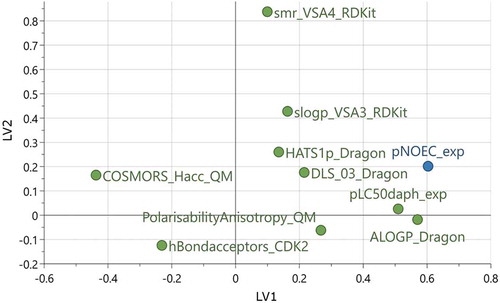
Another important descriptor is the acute toxicity to daphnids (pEC50 daphnid), which has already been observed previously [9,15]. It is the descriptor with the highest correlation to pNOEC (Pearson’s correlation coefficient of 0.67). One substance class exhibiting very high pNOEC and pEC50 daphnid at the same time are the pyrethroids (cypermethrin, deltamethrin, beta-cyfluthrin, acrinathrin, tralomethrin). To exclude spurious bias introduced by this substance class, we tested the effect of removing the pyrethroids from the model but did not observe any significant change on the quality of the model (r² = 0.716, q² = 0.677).

High ability to accept hydrogen-bonds as given by hBondacceptors_CDK2 (count of hydrogen bond acceptor sites) and COSMORS_Hacc_QM (also accounting for H-bond strength, see [45] and references cited therein) reduces a molecule’s pNOEC, presumably by increasing the hydrophilicity. Other empiric rules for drug-likeness of molecules (DLS_03_Dragon, as defined by Walters and Murcko [46]) increase the pNOEC. The PolarizabilityAnisotropy_QM descriptor is related to polarizability and molecular shape. Molecules with high polarizability in one direction and low polarizability in the other directions have high anisotropy values. Usually, these molecules are long and thin and could align well within the lipid bilayer of membranes. Accumulation in membranes is a ubiquitous phenomenon, related to non-polar narcotic toxicity or baseline toxicity. Several other descriptors are related to non-binding weak molecular interactions, especially polarizability and lipophilicity: HATS1p_Dragon is an autocorrelation descriptor weighted by polarizability. slogP_VSA3_RDKit and smr_VSA4_RDKit describe the size of the molecular surface area with a certain range of log P and molecular refractivity, respectively. The latter is related to molecular size and polarizability. Except for pEC50 daphnid, the descriptors indicate rather unspecific mechanisms of toxicity like affinity to membranes or membrane surfaces.

The distribution of the pre-processed descriptor values for the training set varies (see Figure S5). Except for pEC50 daphnid, DLS_03_Dragon, and smr_VSM4_RDKit they show a broad distribution. However, DLS_03_Dragon shows peaks (n = 141) at the positive and smr_VSA4 shows peaks (n = 150) at the negative extreme of the spectrum. This means that drug-likeness (DLS_03) and partial molecular refractivity (smr_VSA4) can be regarded as being similar to indicator variables, assuming only very few different values. The peak around zero of the pEC50 daphnid (n = 61) corresponds to the missing experimental data.

Prediction error and outlier analysis

Figure 5(a) shows the predicted pNOECs of model M6 versus the experimental data from the training set (n = 206) together with their 95% confidence intervals of the predictions and the 95% single prediction confidence intervals according to SIMCA, resulting in a linear fit y = 0.05 + 0.99x. A fit of all 338 compounds, including the 15 compounds outside the AD of the model would result in y = −0.02 + 1.01x. The results for the DEV, VAL, and EXT sets are shown in Figure 5(b). The overall patterns of their confidence intervals or errors do not deviate from that of the training set.

Figure 5. Model M6: Predictions with confidence intervals vs. experiment, for the training set compounds (a) and test sets (b), coloured in red (DEV), blue (VAL), and grey (EXT)

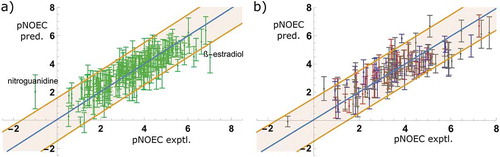
The prediction errors (ΔpNOEC = pNOEC_exptl – pNOEC_pred) of model M6 are normally distributed for all data sets (Figure 6(a)). The two outliers are nitroguanidine at the negative end and ß-oestradiol, a steroid hormone, at the positive end. They will be discussed in the analysis of influential points below. Despite the differentiation between insecticides with many high, herbicides with predominantly low, and fungicides with medium pNOECs (c.f. Figure 1(b)), the errors are independent of their indication (Figure 6(b)). There is no obvious structural pattern common to all the outliers nor is there a characteristic mode of action.

Figure 6. Error distribution of pNOEC predictions by model M6 as counts and normalized distribution functions a) according to set membership and b) for pesticide classes

For estimating the predictivity for future use on chemically related molecules, i.e. crop protection chemicals and their metabolites, we consider the VAL set a representative indicator. The overall performance on this set is comparable to the DEV and cross-validation performance: r²_val of 0.665 and RMSE of 0.820. This set of molecules was only used for testing the final model. It should be noted that it includes 11 of 39 entries with missing pEC50 daphnid data. Performance is slightly higher when only compounds are evaluated for which daphnid data is available (r²_val’ of 0.687 and RMSE of 0.793).

For comparison, we estimated the best hypothetical model performance based on experimental uncertainties from 30 compounds tested on multiple fish species by predicting the single species pNOEC values using the average experimental pNOEC value over all species tested for the respective compound, i.e. predicting experimental outcome using experimental data in the model (see Figure S2 in the SI). From this we calculated an r² of 0.847 and RMSE of 0.514, which can be considered as upper boundary for model performance due to intrinsic variability in the data set and our assumption of negligible inter-species differences. However, taking a single species pNOEC (instead of the mean) to predict the pNOEC of another species would lead to nearly twice as high errors (RMSE = 0.979). That is, for an untested species our model provides a better estimate than taking the pNOEC value of another (tested) species, in cases where no information about the similarity of the species is known.

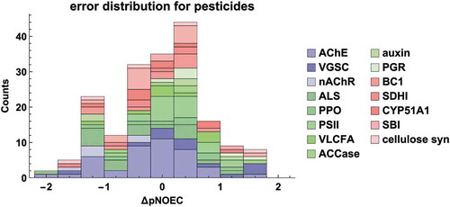
We further investigated the performance of the model with respect to the pesticidal mode of action (MoA, see SI Table S8 for acronyms). More specifically, we analysed MoAs with at least five representatives in the dataset (Figure 7), insecticides (38 x AChE, 13 x VGSC, 6 x nAChR, 3 x VLCFA), herbicides (19 x ALS, 5 x ACCase, 5 x auxins, 6 x growth regulation, 8 x PPO, 22 x PSII, 7 x VLCFA) and fungicides (11 x BC1, 5 x cellulose synthesis, 9 x CYP51A1, 18 x SBI, 7 x SDHI). Due to the paucity of data general MoA-specific statements must be taken with a grain of salt. Nevertheless, it is noteworthy that the highest pNOECs are found to be caused by chemicals acting at the sodium channel (VGSC, see Figure S7 in the Supporting Information). Only for two insecticide classes a trend towards a skewed error distribution can be observed: pNOECs predicted for nAChR agonists are too high and for those binding at the VGSC are too low (see also Figure S7). There is a number of active substances with ΔpNOEC slightly below −1 log unit. These deviations mean that the toxicity towards fish is overestimated, which is in line with a conservative lower tier risk assessment. The number of 15 underestimations (ΔpNOEC > 1) is relatively low, which is remarkable for a model that does not take any prior knowledge about specific toxicity into account. We could not identify any general structural patterns for molecules with high errors. Overall, we conclude that model M6 does not systematically underestimate toxicity for investigated mode of action and thus can be useful for screening-level chronic risk assessments for fish.

Figure 7. Error distribution of pNOEC predictions for pesticides by model M6, coloured according to mode of action (for an explanation of MoA acronyms see SI Table S8, and Figures S6-S8 for histograms on individual MoAs)

Regarding the applicability domain (AD), two of the molecules with the highest pNOEC, i.e. pyrethroid insecticides acting at the voltage-gated sodium channels (VGSC), are outside the AD (acrinathrin and tau-fluvalinate). However, molecules outside the AD of the model can be found at all pNOECs and for various modes of action. For example, the sulphonyl urea herbicides (triflusulfuron-methyl, orthosulfamuron), acting as acetolactate synthase (ALS) inhibitors, and the diamide insecticides (tetraniliprole, flubendiamide), activating the ryanodine receptor, have low pNOECs. At pNOEC range 3–4 we observed the salts (3-dodecyl-1,4-dioxonaphthalen-2-yl) acetate, dodine (fungicide, guanidine salt), the spinosyn spinetoram (nicotinic acetylcholine receptor (nAChR) activator), the organophosphates dichlorvos, ethion and malathion (acetylcholine esterase (AChE) inhibitors), triclosan (polychlorinated phenoxyphenol), acequinocyl (acaricide), 1,3-dichloropropene (a soil fumigant nematicide) and the antiarrhythmic amiodarone to be outside the AD. No obvious trend between mode of action and AD membership can be concluded. Thus, the model is broadly applicable, independent of the mode of action. However, we observed a prevalence for large molecules being outside the AD: 12 out of 338 have a molecular weight above 500 g/mol, of which 6 are outside the AD, i.e. as much as 40% of 15 molecules outside the AD. Applicability must be checked for each molecule individually.

We analysed the influence of the data points on the PLS model by using a Williams plot and a plot of Cook’s distances. Cook’s distance D is a combination of leverage h_i and residual values. It summarizes how much all values in the model change when the single observation i is removed. A Williams plot combines information on unusual responses (outliers) and parameters (high leverage points). The standardized standard residues are plotted against their leverage values where the leverage h_i is the proportion of the total sum of squares of the explanatory variables due to observation i. Compounds with residuals >2.5σ are borderline, those with residuals >3σ are outliers. Definition of a warning leverage, depending on the degrees of freedom, seems to be not trivial for PLS models [47]. Hence, while Cook’s D identifies influential points, Williams plots can differentiate these between good and bad high leverage points.

From Cook’s D (Figure 8), five molecules of the training set are worth a closer inspection: nitroguanidine, the steroid hormone ß-oestradiol, the herbicides glyphosate and maleic hydrazide, and the fungicide cymoxanil. All of them are within the applicability domain of the model, satisfying PModXPS > 0.05. The Williams plot (Figure 9) reveals that nitroguanidine and ß-oestradiol are clearly outliers having standard residues close to 4 σ but relatively small leverages (0.015), the standard residue of cymoxanil is borderline (<2.5 σ), its leverage is small (0.008), while the standard residues of glyphosate and maleic hydrazide (<1.75 σ) and leverages of approximately 0.027 seem to stabilize the model. Excluding these five influential points from the model leads to only minor changes in model parameters and predicted pNOEC (max. 0.1 log units). We therefore did not remove them from the final model.

Figure 8. Cook’s distances for the training and test sets (n = 338) for PLS model M6

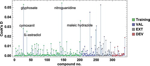
Figure 9. Williams plot with 5 influential training set compounds from Cook’s plot marked

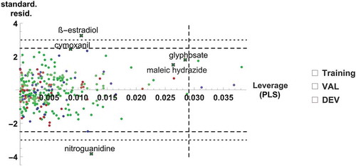
The large error of prediction for nitroguanidine can be satisfactorily explained by the fact that our data table does not contain a corresponding entry for pEC50 daphnid. The missing value is hence replaced by the average pEC50 daphnid. However, in the literature nitroguanidine is reported to be extremely non-toxic to daphnid (pEC50 daphnid > 3 g/L) [48,49]. With this boundary value of 3 g/L, the prediction error is reduced from 3.02 to ≤1.78 log units and would probably be even lower with the exact pEC50. This observation nicely confirms the meaningful structure of our model and the importance of the daphnid EC50 input in particular. Nitroguanidine is of practical importance as a common structural element of the neonicotinoid insecticides.

The other outlier, ß-oestradiol, can be explained by the missing correlation between pEC50 daphnid and pNOEC for the steroids. Fish are extremely sensitive to some steroidal pharmaceuticals [50] and were reported to be at least 1000 times more susceptible than Daphnia and algae to drugs targeting, e.g. sex-steroid receptors, which were not conserved in Daphnia and algae [5]. As the toxicity of ß-oestradiol towards Daphnia is relatively low [51,52], it is erroneously predicted to have a low pNOEC, too. Interestingly, ß-oestradiol is also found to be an outlier in a daphnid-to-chronic fish relationship [9].

The Williams plot in Figure 9 highlights 4 additional molecules as high-leverage points, which however, have low Cook’s D values and therefore are not critical to the model. Two of them are part of the validation set and hence have no influence on the model, while the other two (endothal and endosulfan) are in the training set.

Comparison with existing models

Recently, Furuhama et al. [15] published several QSA(A)R models for FELS based on 77 molecules with experimentally known pNOEC values for fathead minnow and daphnid EC50 values. The models were tested on a set of 36 molecules with pNOEC data for medaka. Here, we compared their models with our model M6 with respect to coverage of chemical space and accuracy of the predictions. Figure 10 shows a t-stochastic neighbour embedding (tSNE) [53] representation of the chemical space covered by our data set with 338 molecules. The training set of Furuhama et al. covers a large fraction of the chemical space of our data set, but some compound classes are not or only sparsely covered. As an example, we could add the herbicidal class of sulfonylureas and the insecticidal class of neonicotinoids, and complement the single representatives of the important fungicidal classes of succinate dehydrogenase (SDH) or cellulose synthesis inhibitors. The medaka test set is narrower and restricted to a small area in that space. It contains mainly ‘normal’ industrial chemicals and very few pesticides. It also spans a narrower range of pNOEC values. We therefore consider our validation set more representative for a broader chemical space. However, for comparison, we predicted both test sets with all models as summarized in Table 4.

Figure 10. Representation of the chemical space covered by the full data set with 338 molecules. We used a t-stochastic neighbour embedding (tSNE) based on Tanimoto distances to embed chemical similarities in two dimensions. Training set (orange) and test set (blue) compounds of the models by Furuhama et al. highlighted in colour

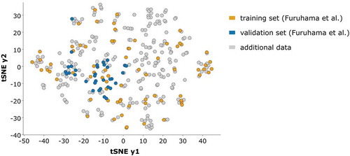
Table 4. Comparison of QSAAR model performance with models by Furuhama et al. [15]

	ID 1 ^a)	ID 2 ^a)	ID 3 ^a)	ID 4 ^a)	Ct432 ^a)	QAAR ^a)	M6 (this work)
RMSEext ^b)	0.89	0.91	0.93	0.87	0.63	0.64	0.62
r^2ext ^c)	0.38	0.39	0.36	0.52	0.56	0.56	0.63
Q^2ext ^d)	0.16	0.12	0.09	0.20	0.58	0.57	0.57
z > 1.0 ^e)	8	8	7	6	2	2	1
RMSEVAL‘ ^f)	1.04	0.99	1.14	1.27	1.14	1.20	0.79
r^2VAL‘ ^f)	0.50	0.54	0.40	0.26	0.39	0.28	0.69
no. of variables	8	9	9	7	2	1	9
proprietary software required	yes	yes	yes	yes	no	no	yes

^aID 1–4, Ct432, QAAR are models with the lowest errors from ref [15]. Results in rows 1–4 were taken from the original article for comparison.

^bRMSE_ext, root mean square error on validation set from ref [15].

^cr²_ext, squared correlation coefficient between measured and estimated pNOEC on validation set from ref [15].

^dQ²_ext, external explained variance on validation set as given in ref [15].

^ez > 1.0, number of underestimates by more than 1 log unit on validation set from ref [15].

^fRMSE_VAL’, r²_VAL’ on validation set from this work, excluding compounds with missing values for daphnids. 4 chemicals were present in the training set of models ID1-4, Ct432, QAAR.

‘QAAR’ is a linear regression on experimental Daphnia pEC50 values, Ct432 extends that model with a Toxprint Chemotype [54], and ‘ID 1–4ʹ are linear QSAAR models based on 7–9 descriptors including Daphnia pEC50, log D from ACD/Labs, and σ-moments from COSMO-RS calculations. On the medaka test set from ref [15]., we achieved a root mean square error of 0.616, which is lower than the models previously reported. Additionally, the number of underestimates could be reduced to 1, which is an important metric to inform risk assessments. Removing the 19 molecules that were part of our training set for fairer comparison, left the RMSE basically unchanged at 0.620. On our VAL set, all models have higher RMSE, which reflects the higher difficulty to predict a more diverse chemical space and a larger range of response values. The best predictivity on this set was achieved with model M6, although the other models used 4 of the molecules in their training set. The complexity of the models as well as the availability and computational costs of the descriptors are similar. The only exceptions are QAAR and Ct432, which have only 1 or 2 variables and do not require proprietary software but show inferior performance on diverse sets like the VAL or even their own training sets (RMSE of 1.18 and 1.11, respectively). In conclusion, model M6 improved predictivity and is more broadly applicable.

Availability

To facilitate model predictions, we provide a KNIME workflow on KNIME Hub, which automatically performs the pre-processing of molecular structures given as SMILES strings, pre-processes the descriptors and applies model equation M6 to obtain the final prediction. In general, for QSAR models it is important to ensure consistent results. This includes using the same software versions and identical structure pre-processing. We checked the consistency of the predictions with KNIME v4.2.0 [32], RDKit KNIME integration 4.0.1.v202006261025 [26], and CDK 2.3 [31]. We also included a data table in the workflow, which can be used for testing the reproducibility of our predictions.

Conclusions

With the aim to develop new predictive models, we compiled the so far largest data set on FELS NOEC endpoints for 338 molecules, based on internal studies and public data sources. The larger data set extended the chemical space and applicability domain of previous models and led to more powerful statistics for model development and validation. We used partial least squares techniques (PLS, sPLS) which are known to be robust with respect to collinearity in the descriptor variables and applicable to the p > n problem with more variables than observations. Preselection of variables with the help of sparse PLS and fine tuning by expert knowledge led to a reasonably simple PLS model consisting of two latent variables from 8 molecular descriptors and experimental acute toxicity towards Daphnia magna. Most important descriptors are lipophilicity (ALOGP) and pEC50 daphnid, which is correlated to FELS NOEC as reported earlier [9,15]. Additionally, two descriptors obtained from density functional theory and the COSMO-RS solvent model supported predictivity by a more accurate description of molecular interaction properties. This new PLS model is broadly applicable and provides better statistical performance than previous models, with an r² of 0.687 and an RMSE of 0.793 log units on a representative test data set of chemically related molecules with available experimental Daphnia magna data. Its prediction errors are normally distributed and consistent. Hence, we did not find any model failures in terms of systematic underestimation of toxicity regarding pesticidal modes of action or with regard to structural patterns. The model is available as a KNIME workflow for the pre-processing of molecular structures and descriptors as well as prediction of NOEC values.

We see potential applications of the model in prioritization of chemicals for testing, such that only chemicals are tested for which higher precision is of importance for risk assessments. It could also support the development of new crop protection active ingredients, and the planning of studies. Future research might focus on the following topics. Besides adding more data for fish NOEC and daphnid EC50, a better imputation method for the daphnid pEC50 could be beneficial. It might even be possible to replace the experimental value with a robust QSAR for the daphnid endpoint, such that fish NOEC prediction becomes independent from experimental data. In the long term, it might also be possible to develop models for individual effects for the different life stages or to investigate whether the approach can be extended to predict EC10 endpoints.

Acknowledgements

We thank Michael Kohnen, Svend Matthiesen, and Michael E. Beck for access to and support with the high-performance compute infrastructure, as well as Zhenglei Gao, Eric Bruns, and Steven Levine for helpful discussions and critically reading the manuscript.

Data availability Statement

The data that support the findings of this study are openly available via figshare at http://doi.org/10.6084/m9.figshare.c.5194022. The model workflow is available in KNIME Hub at https://kni.me/w/CEyXPUo_n1i4pUiR.

Disclosure statement

The authors are employees of Bayer AG, a manufacturer of pharmaceuticals, agricultural, and consumer health chemicals.

Supplementary material

Supplementary data for this article can be accessed at: https://doi.org/10.1080/1062936X.2021.1874514.

References

- Test No. 210: Fish, early-life stage toxicity test. OECD Guidelines for the Testing of Chemicals, Section 2, OECD Publishing, Paris, 2013.
- N. Choudhury, Ecotoxicology of aquatic system: A review on fungicide induced toxicity in fishes, Pro. Aqua Farm. Marine Biol. 1 (2018), pp. 180001–180005.
- K.R. Solomon, K. Dalhoff, D. Volz, and G. van der Kraak, Effects of herbicides on fish, in Fish Physiology, K.B. Tierney, A.P. Farrell, and C.J. Brauner, eds., Academic Press, London, 2013, pp. 369–409.
- M.H. Fulton, P.B. Key, and M.E. DeLorenzo, Insecticide toxicity in fish, in Fish Physiology, K.B. Tierney, A.P. Farrell, and C.J. Brauner, eds., Academic Press, London, 2013, pp. 309–368.
- L. Gunnarsson, J.R. Snape, B. Verbruggen, S.F. Owen, E. Kristiansson, L. Margiotta-Casaluci, T. Österlund, K. Hutchinson, D. Leverett, B. Marks, and C. Tyler, Pharmacology beyond the patient – The environmental risks of human drugs, Environ. Int. 129 (2019), pp. 320–332. doi:10.1016/j.envint.2019.04.075.
- S. Ullah and J. Zorriehzahra, Ecotoxicology: A review of pesticides induced toxicity in fish, Adv. Anim. Vet. Sci. 3 (2014), pp. 40–57. doi:10.14737/journal.aavs/2015/3.1.40.57.
- M. Halder, A. Kienzler, M. Whelan, and A. Worth, EURL ECVAM Strategy to Replace, Reduce and Refine the Use of Fish in Aquatic Toxicity and Bioaccumulation Testing, Publications Office of the European Union, Luxembourg, 2014.
- M. May, W. Drost, S. Germer, T. Juffernholz, and S. Hahn, Evaluation of acute-to-chronic ratios of fish and Daphnia to predict acceptable no-effect levels, Environ. Sci. Eur. 28 (2016), pp. 16. doi:10.1186/s12302-016-0084-7.
- A. Kienzler, M. Halder, and A. Worth, Waiving chronic fish tests: Possible use of acute-to-chronic relationships and interspecies correlations, Toxicol. Environ. Chem. 99 (2017), pp. 1129–1151. doi:10.1080/02772248.2016.1246663.
- S. Scholz, R. Schreiber, J. Armitage, P. Mayer, B.I. Escher, A. Lidzba, M. Léonard, and R. Altenburger, Meta-analysis of fish early life stage tests—Association of toxic ratios and acute-to-chronic ratios with modes of action, Environ. Toxicol. Chem. 37 (2018), pp. 955–969. doi:10.1002/etc.4090.
- K. Mayo-Bean, K. Moran, B. Meylan, and P. Ranslow, Ecological Structure - Activity Relationships Program (ECOSAR) Methodology Document V2.0, US Environmental Protection Agency, Washington, DC, USA, 2017.
- E.M. de Haas, T. Eikelboom, and T. Bouwman, Internal and external validation of the long-term QSARs for neutral organics to fish from ECOSARTM, SAR QSAR Environ. Res. 22 (2011), pp. 545–559. doi:10.1080/1062936X.2011.569949.
- L. Claeys, F. Iaccino, C.R. Janssen, P. van Sprang, and F. Verdonck, Development and validation of a quantitative structure–activity relationship for chronic narcosis to fish, Environ. Toxicol. Chem. 32 (2013), pp. 2217–2225. doi:10.1002/etc.2301.
- T.J. Austin and C.V. Eadsforth, Development of a chronic fish toxicity model for predicting sub-lethal NOEC values for non-polar narcotics, SAR QSAR Environ. Res. 25 (2014), pp. 147–160. doi:10.1080/1062936X.2013.871577.
- A. Furuhama, T.I. Hayashi, and H. Yamamoto, Development of models to predict fish early-life stage toxicity from acute Daphnia magna toxicity, SAR QSAR Environ. Res. 29 (2018), pp. 725–742. doi:10.1080/1062936X.2018.1513423.
- I. Halleux, N. Bornatowicz, B. Grillitsch, K. Delbeke, C. Janssen, G. Atkinson, P. Delorme, D. Moore, C. Hansen, H. Holst, G. Akkerhuis, N. Nyholm, H. Braunschweiler, J. Férard, E. Vindimian, A. Lange, S. Martin, T. Ratte, M. Streloke, S. Marchini, J. Badeaux, R. Bogers, C. Leeuwen, E. Spikkerud, E. Moliner, B. Dahl, L. Lindqvist, R. Fisch, M. Crane, J. Fenlon, A. Riddle, T. Sparks, R. Clements, D. Farrar, M. Newman, M. Harras, R. Maisch, J. Jaworska, R. Egmond, K. Steward, L. Tattersfield, K. Romijn, P. Isnard, G. Joermann, B. Kooijman, J.T. Meister, L. Touart, P. Chapman, S. Park, N. Grandy, and M. Huet, Report of the OECD Workshop on Statistical Analysis of Aquatic Toxicity Data, 1998.
- D.R. Fox, E. Billoir, S. Charles, M.L. Delignette-Muller, and C. Lopes, What to do with NOECS/NOELS—prohibition or innovation? Integr. Environ. Assess. Manag. 8 (2012), pp. 764–766. doi:10.1002/ieam.1350.
- EFSA - European Food Safety Authority, Guidance on tiered risk assessment for plant protection products for aquatic organisms in edge‐of‐field surface waters, Efsa J. 11 (2013), pp. 1–268.
- ECHA - European Chemicals Agency, Guidance on information requirements and chemical safety assessment (Chapter R.11: PBT/vPvB assessment), 2017.
- A. Rácz, D. Bajusz, and K. Héberger, Modelling methods and cross-validation variants in QSAR: A multi-level analysis, SAR QSAR Environ. Res. 29 (2018), pp. 661–674. doi:10.1080/1062936X.2018.1505778.
- J.A. Wegelin, A survey of partial least squares (PLS) methods, with emphasis on the two-block case, Technical Report No. 371, University of Washington, USA, 2000.
- M. Fernández-Delgado, M.S. Sirsat, E. Cernadas, S. Alawadi, S. Barro, and M. Febrero-Bande, An extensive experimental survey of regression methods, Neural Netw. 111 (2019), pp. 11–34. doi:10.1016/j.neunet.2018.12.010.
- A. Bassan, L. Ceriani, J. Richardson, A. Livaniou, A. Ciacci, R. Baldin, S. Kovarich, E. Fioravanzo, M. Pavan, D. Gibin, G. Di Piazza, L. Pasinato, S. Cappé, H. Verhagen, T. Robinson, and J. Dorne, OpenFoodTox: EFSA’s chemical hazards database, Version 2, 2018. doi:10.5281/zenodo.1252752.
- S.D. Dimitrov, R. Diderich, T. Sobanski, T.S. Pavlov, G.V. Chankov, A.S. Chapkanov, Y.H. Karakolev, S.G. Temelkov, R.A. Vasilev, K.D. Gerova, C.D. Kuseva, N.D. Todorova, A.M. Mehmed, M. Rasenberg, and O.G. Mekenyan, QSAR Toolbox – Workflow and major functionalities, SAR QSAR Environ. Res. 27 (2016), pp. 203–219. doi:10.1080/1062936X.2015.1136680.
- S.E. Belanger, J.M. Rawlings, and G.J. Carr, Use of fish embryo toxicity tests for the prediction of acute fish toxicity to chemicals, Environ. Toxicol. Chem. 32 (2013), pp. 1768–1783. doi:10.1002/etc.2244.
- RDKit: Open-source cheminformatics; http://www.rdkit.org. 2020.
- Schrödinger Release 2019-1: LigPrep and MacroModel, Schrödinger, LLC, New York, NY, 2019.
- TURBOMOLE V7.0.1. A development of University of Karlsruhe and Forschungszentrum Karlsruhe GmbH, 1989-2007, TURBOMOLE GmbH, since 2007, 2016. available from: http://www.turbomole.com.
- F. Eckert and A. Klamt, Fast solvent screening via quantum chemistry: COSMO-RS approach, AIChE J. 48 (2002), pp. 369–385. doi:10.1002/aic.690480220.
- F. Eckert and A. Klamt, COSMOtherm, Version C3.0, Release 16.01, COSMOlogic GmbH & Co KG, Leverkusen, Germany, 2015.
- J. Mayfield, E. Willighagen, R. Guha, G. Torrance, K. Ujihara, S.A. Rahman, J. Alvarsson, M.B. Vine, S. Grazulis, T. Pluskal, Y.C. Wei, D. Szisz, M.J. Williamson, N. Kochev, N. Jeliazkova, E. Bach, A. Berg, A. Clark, R. Stephan, M. Wenk ficolas2, O. Stueker, K. Dole, K. Jönsson kaibioinfo, L. Burgoon, D. Katsubo, A. Howlett, U. Köhler, and C. Harmon, CDK 2.3, 2019.
- M.R. Berthold, N. Cebron, F. Dill, T.R. Gabriel, T. Kötter, T. Meinl, P. Ohl, C. Sieb, K. Thiel, and B. Wiswedel, KNIME: The konstanz information miner, in Studies in Classification, Data Analysis, and Knowledge Organization (GfKL), 2007.
- Sybyl Version X 2.1 – Discovery Software for Computational Chemistry and Molecular Modelling, including UNITY fingerprint tools. distributed by Tripos Inc., St. Louis, MO, USA, 2004.
- Dragon v7.0: Software for molecular descriptor calculation. Kode Chemoinformatics, 2017.
- C.W. Yap, PaDEL-descriptor: An open source software to calculate molecular descriptors and fingerprints, J. Comput. Chem. 32 (2011), pp. 1466–1474. doi:10.1002/jcc.21707.
- A. Mauri, alvaDesc: A tool to calculate and analyze molecular descriptors and fingerprints, in Ecotoxicological QSARs. Methods in Pharmacology and Toxicology, K. Roy, ed., Humana, New York, NY, 2020, pp. 801–820.
- M. Ashton, J. Barnard, F. Casset, M. Charlton, G. Downs, D. Gorse, J. Holliday, R. Lahana, and P. Willett, Identification of diverse database subsets using property-based and fragment-based molecular descriptions, Quant. Struct-Act. Rel. 21 (2002), pp. 598–604. doi:10.1002/qsar.200290002.
- S. Wold, M. Sjöström, and L. Eriksson, PLS-regression: A basic tool of chemometrics, Chemom. Intell. Lab. Syst. 58 (2001), pp. 109–130. doi:10.1016/S0169-7439(01)00155-1.
- SIMCA 16, Sartorius Stedim Data Analytics AB, Umeå, Sweden, 2020. www.sartorius.com/umetrics.
- K.-A. Lê Cao, D. Rossouw, C. Robert-Granié, and P. Besse, A sparse PLS for variable selection when integrating omics data, Stat. Appl. Genet. Mol. Biol. 7 (2008), pp. 1–29. doi:10.2202/1544-6115.1390.
- K.-A. Lê Cao, F. Rohart, I. Gonzalez, S. Dejean, B. Gautier, F. Bartolo, P. Monget, J. Coquery, F. Yao, and B. Liquet, MixOmics: Omics data integration project. R Package Version 6.1.1., 2016. https://CRAN.R-project.org/package=mixOmics.
- A.K. Ghose and G.M. Crippen, Atomic physicochemical parameters for three-dimensional structure-directed quantitative structure-activity relationships I. Partition coefficients as a measure of hydrophobicity, J. Comput. Chem. 7 (1986), pp. 565–577. doi:10.1002/jcc.540070419.
- V.N. Viswanadhan, A.K. Ghose, G.R. Revankar, and R.K. Robins, Atomic physicochemical parameters for three dimensional structure directed quantitative structure-activity relationships. 4. Additional parameters for hydrophobic and dispersive interactions and their application for an automated superposition of certain naturally occurring nucleoside antibiotics, J. Chem. Inform. Comput. Sci. 29 (1989), pp. 163–172.
- A. Gissi, A. Lombardo, A. Roncaglioni, D. Gadaleta, G.F. Mangiatordi, O. Nicolotti, and E. Benfenati, Evaluation and comparison of benchmark QSAR models to predict a relevant REACH endpoint: The bioconcentration factor (BCF), Environ. Res. 137 (2015), pp. 398–409. doi:10.1016/j.envres.2014.12.019.
- K. Wichmann, M. Diedenhofen, and A. Klamt, Prediction of blood-βrain partitioning and human serum albumin binding based on COSMO-RS σ-Moments, J. Chem. Inf. Model. 47 (2007), pp. 228–233. doi:10.1021/ci600385w.
- W.P. Walters and M.A. Murcko, Prediction of ‘drug-likeness, Adv. Drug Deliv. Rev. 54 (2002), pp. 255–271. doi:10.1016/S0169-409X(02)00003-0.
- N. Krämer and M. Sugiyama, The degrees of freedom of partial least squares regression, J. Am. Stat. Assoc. 106 (2011), pp. 697–705. doi:10.1198/jasa.2011.tm10107.
- W.H. van der Schalie, The Toxicity of Nitroguanidine and Photolyzed Nitroguanidine to Freshwater Aquatic Organisms, Army Medical Bioengineering Research and Development Lab Fort Detrick, Frederick, Maryland, 1985.
- REACH registration dossier for 1-nitroguanidine, registration number 01-2119489412-35-0002, 2020. accessed 24 May 2020. https://echa.europa.eu/registration-dossier/-/registered-dossier/13550/6/2/4/?documentUUID=2c157e51-4cba-4bcf-81f5-7b48becf2c11.
- T.J. Thrupp, T.J. Runnalls, M. Scholze, S. Kugathas, A. Kortenkamp, and J.P. Sumpter, The consequences of exposure to mixtures of chemicals: Something from ‘nothing’ and ‘a lot from a little’ when fish are exposed to steroid hormones, Sci. Total Environ. 619–620 (2018), pp. 1482–1492. doi:10.1016/j.scitotenv.2017.11.081.
- R.L. Clubbs and B.W. Brooks, Daphnia magna responses to a vertebrate estrogen receptor agonist and an antagonist: A multigenerational study, Ecotoxicol. Environ. Saf. 67 (2007), pp. 385–398. doi:10.1016/j.ecoenv.2007.01.009.
- Beta-Estradiol EQS Dossier, 2011. https://circabc.europa.eu/sd/a/c5356fa7-be0e-4d3b-b199-208d6e144a91/E2%20EQS%20dossier%202011.pdf
- L.J.P. van der Maaten and G.E. Hinton, Visualizing high-dimensional data using t-SNE, J. Mach. Learn. Res. 9 (2008), pp. 2579–2605.
- C. Yang, A. Tarkhov, J. Marusczyk, B. Bienfait, J. Gasteiger, T. Kleinoeder, T. Magdziarz, O. Sacher, C. Schwab, J. Schwoebel, L. Terfloth, K. Arvidson, A. Richard, A. Worth, and J. Rathman, New publicly available chemical query language, CSRML, to support chemotype representations for application to data mining and modeling, J. Chem. Inf. Model. 55 (2015), pp. 510–528. doi:10.1021/ci500667v.