Comparing Regional Patterns of Individual Movement Using Corrected Mobility Entropy

ABSTRACT

In this paper, we propose a correction of the Mobility Entropy indicator (ME) used to describe the diversity of individual movement patterns as can be captured by data from mobile phones. We argue that a correction is necessary because standard calculations of ME show a structural dependency on the geographical density of observation points, rendering results biased and comparisons between regions incorrect. As a solution, we propose the Corrected Mobility Entropy (CME). We apply our solution to a French mobile phone dataset with ∼18.5 million users. Results show CME to be less correlated to cell-tower density (r = –0.17 instead of –0.59 for ME). As a spatial pattern of mobility diversity, we find CME values to be higher in suburban regions compared to their related urban centers, while both decrease considerably with lowering urban center sizes. Based on regression models, we find mobility diversity to relate to factors like income and employment. Additionally, using CME reveals the role of car use in relation to land use, which was not recognized when using ME values. Our solution enables a better description of individual mobility at a large scale, which has applications in official statistics, urban planning and policy, and mobility research.

KEYWORDS:

• Mobility Entropy
• CDR data
• mobility studies
• regional geography
• urban areas

Introduction

The study of large-scale human movement has benefitted greatly from advances in information technologies, allowing for the collection of data on individual movement for large-scale populations. Traditional approaches, such as interviews, questionnaires, and travel diaries are ill-suited to study large populations because they require considerable effort from both researchers and participants, which in turn results in datasets with smaller sample sizes, limited observation periods, and even incomplete information (Chen et al., 2014; Janzen et al., 2016; Janzen et al., 2018). In contrast, modern technologies like GPS, Location-Based Services (LBS), Location-Based Social Networks (LBSN), Online Social Networks (OSN), and mobile phone data, are all capable of passively sensing individual movement for large groups of individuals and at high spatio-temporal resolution. As a consequence, datasets captured by these technologies have been widely deployed to study large-scale human mobility patterns (Bojic et al., 2015; Chen et al., 2014; Pappalardo et al., 2013; Wolf et al., 2001). The contribution to the literature is that they have allowed for the derivation of several statistical properties of large-scale human mobility, e.g., power-law distributions of displacements, mobility motifs, visitation frequency, and staying time (González et al., 2008; Song, Koren, et al., 2010; Song, Qu, et al., 2010; Szell et al., 2012; Wang et al., 2014) and they have inspired works that try to model the observed empirical properties (Kang et al., 2012; Noulas et al., 2012; Simini et al., 2012). One downside of datasets with large samples of individuals is that their investigation tends to presume universality of the observed empirical properties. Consequently, these works are, either implicitly or explicitly, advocating a disputable universality of human movement leading to a generalist and limited view of human mobility (Schwanen, 2016).

The presumption of universality in human mobility opposes decades of (geographical) research that has been focusing on the particularity of individual movement and the (geographical) context in which it is situated (Schwanen, 2016). Individual mobility, for instance, is influenced by a wide range of constraints, including socioeconomic characteristics and the direct environment (Asgari et al., 2013), which differ between individuals as well as between geographical regions (given that constraints can be common for larger populations). The problem with positivist, empiricist approaches is not necessarily that they fail to address particularity; as a posteriori confrontation with context-situated insights might benefit both strands of research (Beckers et al., 2017). It is that they fail to recognize how their methodological canon is erasing particularity (or when it comes to large-scale mobility: geographical heterogeneity), leading to limited insights, unthoughtful application, and even the use of incorrect methodologies.

In this paper, we address a clear example of such an “incorrect” methodology. We show how the canonically used Mobility Entropy (ME), an indicator for the diversity of individual movement, by design fails to incorporate geographical heterogeneity. Consequently, it cannot be used for objective comparison at the scale of regions or even urban areas. We find that the standard calculation of ME is dependent on the geographical density of observations points,¹ leading to similar movement patterns to have higher values of ME in areas with higher densities of observation points. In the case of Call Detailed Record (CDR) CDR data, for example, regions with high densities of cell-towers, like cities or popular tourist destinations, will by definition depict higher ME values. Other data collection technologies, like OSN or LBS, are equally prone to this problem given that they too display structural differences in observation point density (check-in locations and locations of service use respectively).

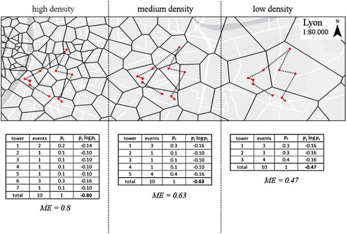
Figure 1 illustrates the problem, showing how the same movement pattern results in different ME values for areas A, B, C, which are characterized by a decreasing density of observation points. The obtained mobility entropy values differ significantly because the resolution of information derived from the cell-tower network is different. The implication is an ME indicator that is spatially biased when densities of observation points are different, resulting in incorrect spatial distributions of ME values. Consequently, ME values form a non-objective indicator for comparison between regions, all the while affecting interpretations, applications, and models that are based on them.

Figure 1. Illustration of the effect of different cell-tower densities on the calculation of the temporally-uncorrelated mobility entropy (ME) Mobility entropy for the same path (dotted line) of a user in three different density settings is calculated and shown to be different

As a solution, we propose an adaptation of the standard ME to what we call the Corrected Mobility Entropy (CME). We elaborate our proposition based on individual movement patterns of almost 18.5 million users captured in a CDR dataset by the French telecom operator Orange. Our main results consist of a comparison between ME and CME values. We show how locally aggregated CME values (1) are less correlated to cell-tower densities, (2) depict different spatial patterns for regions as well as functional urban areas as defined by the French Statistics Office, and (3) have different relations to mobility-related indicators collected nation-wide by census or remote sensing. Our findings urge the research community to reconsider the use of the standard ME indicator, especially when comparing geographical regions with clear structural differences in observation point density.

Related Work

Capturing Large-Scale Movement Patterns with CDR Data

Call Detail Records (CDR) data are the most basic examples of mobile phone data. They are generated as a byproduct of mobile phone activity and stored by the network provider for billing or maintenance purposes. CDRs contain metadata of each interaction (call or text) of the subscriber with the operator’s network, including location data at the level of the contacted cellular tower. Based on CDR data, movement patterns of individuals can be re-constructed at cell-tower network resolution and with the temporal granularity of a user’s cell phone activity. The main difficulty in this perspective are sporadic observations for certain users and differing accuracy of location detection with changing tower density (Ranjan et al., 2012; Tanahashi et al., 2012).

CDR data have extensively been used to study large-scale human mobility patterns (Kung et al., 2014; Ranjan et al., 2012; Simini et al., 2012), population presence (Deville et al., 2014), and other topics.² The real strength of CDR data with relation to mobility is its ability to capture movement on a fine-grained resolution for populations of, often, millions of users. Compared to the gathering of other data, the gathering of CDR data is more cost-effective, less biased, and available on a much larger scale in terms of users, geographical coverage, and time periods compared to traditional data gathering methods (Järv et al., 2014; Liu et al., 2013), while collected at the individual level, CDR data still allows for a reconstruction and quantification of individual movement patterns. As a consequence, indicators for individual mobility, like the number of visited cell-towers, the radius of gyration, or the mobility entropy, have been derived from mobile phone data and are used to inform large-scale studies on, for instance, the mobility footprint of users (Sridharan and Bolot, 2013), mobility differences between population groups (Bajardi et al., 2015; Cranshaw et al., 2010), or the relation between mobility and poverty (Pappalardo et al., 2016).

Defining the Mobility Entropy (ME) Indicator

In this paragraph, we focus on the Mobility Entropy (ME) indicator. An exact definition of mobility entropy is provided for in the following paragraphs but an intuitive interpretation can already be formulated: mobility entropy is the uncertainty of location visits or, in other terms, the diversity of visited locations by an individual mobile phone user.

The standard definition of mobility entropy is based on the entropy concept developed by Claude Shannon in his seminal work: A Mathematical Theory of Communication. In this work, Shannon discusses the transmission of messages through a system as a sequence of transitions in a Markov chain. Due to the different transition probabilities in such a Markov chain, an uncertainty of the next transition can be calculated. Here is where the Shannon entropy was introduced. Based on the probabilities associated with the possible transitions of one state in a Markov chain to another, at each transition an entropy value could be calculated, representing the rate at which new information is produced (Shannon, 2001 [1948]).

The formula for entropy is rather simple; at least in comparison to the complexity of the system it is trying to characterize (Equation 1). The base of the logarithm can vary. Shannon used base two as he was studying communication systems that depend on bits. In this paper, base ten will be used, following the example of other mobility-related works in the literature (Lin et al., 2012; de Montjoye et al., 2016; Pappalardo et al., 2016); resulting in the decimal entropy (H). One can interpret the formula as a counteracting between the probability of a state (p_i) and its own logarithm (log(p_i)) resulting in a function (H) reaching a maximum when equal probabilities are observed for all states.(1)

The Shannon entropy can be applied to several systems, including individual movement patterns, to serve as a measure for the degree of predictability. In a movement pattern perspective, each visited location equals a state and the probability of being in a state, ideally, equals the time a user spends in this location. The mobility entropy, hence, becomes the degree of predictability of the movement pattern of a person or, conversely, the diversity of an individual movement pattern.

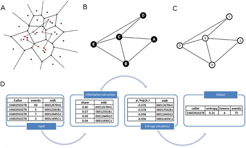
Applying Shannon’s entropy to individual movement patterns derived from CDR data, Song, Qu et al. (2010) propose three different ways of calculating mobility entropy: (1) random entropy, (2) temporally-uncorrelated entropy and (3) real entropy. For all three measures, locations (and thus states of the systems) are based on the visited cell-towers. However, the probabilities of being in a certain state (at a certain cell-tower) are calculated differently and are provided by (1) whether the user visited the cell-tower before or not, (2) the number of times the user visited a cell-tower and (3) the actual time spent by a user in the area of a cell-tower. The last of which, (3), is not obtainable given the sparse temporal resolution of most users in the CDR dataset and given that the first neglects to take full advantage of the available information in the CDR dataset, we will continue this work by using the temporally-uncorrelated entropy only (2). The full equation of the temporally-uncorrelated entropy is given in Equation 2, and a graphic illustration of its calculation for one user in the dataset is given in Figure 2.(2) Remember that the problem statement of our paper is that the standard calculation of ME, as defined in Equation 2 incorporates a bias because of its dependency on the number of observation points (or thus cell-towers in the case of CDR data) in an area. Higher numbers of observations points (cell-towers) lead to higher values for n and lower values for p_i both combined resulting in higher values for ME.

Figure 2. Graphic illustration for the calculation of mobility entropy from CDR data. (A) The actual path a user follows in space (dotted lines) and the events he initiates (red dots) at cell-towers (black dots). The Voronoi polygons (full lines) represent the service area borders of the different cell phone. (B) The mobility network based on the visited towers. This representation accords with the random entropy in Song et al., 2010b. (C) The mobility network based on the number of visits to the towers. This representation accords with the temporal-uncorrelated entropy in Song et al., 2010b and will be used throughout the rest of the work. (D) Database representation of the different steps to calculate the temporal-uncorrelated mobility entropy for one user with unique identifiers of cell-tower locations

Mobility Entropy and Uncertain Predictability of Human Mobility

The real breakthrough of mobility entropy in literature came with the seminal paper by Song, Qu et al. (2010). They show that, for a three-month long CDR dataset of 45,000 users (selected on amount of activities), the distribution of real entropy values peaks at 0.8. Using a log with base 2 this indicates the expected uncertainty of the next visited location by a person to be 2^0.8= 1.78 or thus fewer than two locations. Building further on this finding they establish an explicit formula for the upper bound of predictability of human movement patterns, and find a surprising 93 percent of potential predictability in their dataset; meaning that “despite the apparent randomness of the individuals’ trajectories, a historical record of the daily mobility pattern of the users hides an unexpectedly high degree of potential predictability” (Song, Qu et al., 2010: 1020).

Stimulated by this finding and guided by statistical properties empirically derived from large-scale records of human movement, e.g., the distribution of displacements (Cheng et al., 2011; Kang et al., 2012; Yan et al., 2013), a large number of predictive models for human mobility have recently been developed. Such models take into account different influencing aspects, ranging from population characteristics (Gonzalez et al., 2008) and individuals’ activities (Song, Koren, et al., 2010) to geographical environments (Kang et al., 2012), and distance effects (Noulas et al., 2012; Simini et al., 2012), hereby shedding different lights on what actually makes up the supposed predictability of human movement (Liu et al., 2014).

As these models have become significantly more advanced, covering finer resolutions of space and time, some works have been directed to understanding the sensitivity of predictability to different spatial and temporal scales (Jensen et al., 2010; Lin et al., 2012; Smith et al., 2014), different data collection techniques (Jensen et al., 2010) and practical limitations like topological characteristics (Smith et al., 2014). Until 2012, predictability changes with respect to different spatial/temporal scales were largely unknown (Lin et al., 2012). Investigating this sensitivity, Lin et al. find a “rather linear [positive] relation” between scale and the predictability upper bound for eight individuals tracked with high-resolution GPS. This finding is in line with Smith et al. (2014), who strongly challenge assumed upper bounds in literature arguing that they do not consider real-world topological characteristics. Taking into account topological constraints, they too find that predictability relates to scale but this time “almost exponentially” (Smith et al., 2014).

The sensitivity of movement predictability to spatial scale bears two consequences. First, it means that human movement is potentially less predictable than had been previously assumed. With respect to predictive models, this means that incorporation of variables other than location information, as well as good insights in how predictability is distributed among populations, will most likely be needed to improve prediction performance. The former has been proposed by several lines of work that suggest that knowledge about social networks might improve mobility prediction (Cho et al., 2011; De Domenico et al., 2013; Phithakkitnukoon et al., 2012; Toole et al., 2015). Concerning the latter, there has been a recent rise in studies investigating the relationship between mobility indicators (like ME) and mobile phone usage (Lu et al., 2017; Zhao et al., 2016), demographics (Yuan and Raubal, 2016), economic indicators (Bajardi et al., 2015; Pappalardo et al., 2016), social-temporal orders (Yuan et al., 2012), and even the built environment (Yuan et al., 2012; Yuan and Raubal, 2016). Similar investigations existed before, but were mostly done on much smaller sample sets. ME, for instance, has been used in individual activity tracking to obtain insights in its temporal differences (day, night, week, weekend) (Cho et al., 2011) as well as between population groups (Cranshaw et al., 2010).

The sensitivity of movement predictability to spatial scale means that differences in spatial scale result in a problematic comparison of mobility traces. Lin et al. (2012: 386) noted this volatility when their experiments suggested “changing temporal scales has similar effects on the predictability of different individuals, while changing the spatial scale has different effects, depending on the mobility characteristics of each individual.” Osgood et al. (2016: 3) state:

comparing different individuals in the same dataset could be problematic if there is heterogeneity in the geographic bin size or sampling rate; for example, in a study comparing the mobility of rural and urban populations through cell phone records, where the rural Voronoi cells were systemically and significantly larger than their urban counterparts.

Osgood et al. (2016) are, to the best of the authors’ knowledge, the first and only to provide a theoretical derivation of a scaling law for mobility entropy. Using Lempel-ziv compression on non-repeating straight-line paths to estimate mobility entropy, they show how ME’s scaling behavior can be described by four terms: the length of the path, the average velocity of the agent, the width of the spatial bin, and the period of the sampling rate. Despite several assumptions and the limited applicability of their current approach, they show that a theoretical solution for the spatial heterogeneity problem should be feasible in the future.

In the next few paragraphs, we demonstrate how the heterogeneity of spatial scales affects the calculation of ME for a large CDR dataset in France. Our contribution is twofold. First, we are the first to address the problem in an applied, explicitly spatial way; seeking to understand how the heterogeneity of spatial scales results in a wrongful depiction of mobility (predictability) in the French territory and how this misinformation relates to larger regions, like urban areas. Second, we propose an easy solution that exists in correcting the standard ME formula to minimize dependency on the density of observation points that is responsible for the heterogeneity of spatial scales in the first place. Although our solution is difficult to validate and will certainly not be as elegant as theoretical solutions worked out in the future, it serves well in unveiling the spatial aspects and extent of the problem.

Defining Corrected Mobility Entropy (CME)

To balance the influence of cell-tower density on ME we propose a simple, yet effective, normalization of the entropy formula for cell-tower density. Existing entropy normalization, like that done in the Python toolbox “bandicoot,” consists of dividing the entropy by the logarithm of either the number of visited towers or the number of events (de Montjoye et al., 2016). Such approach might seem promising but in fact corrects for the amount of actions on the cell-tower, not for the distribution of cell-towers. For this reason our proposition focuses on the correction of each cell-tower in the entropy formula based on its surrounding cell-tower density. The formula for Corrected Mobility Entropy (CME) then becomes:(3) The idea behind the proposed correction is straightforward. When cell-tower density is high, visiting a new cel0l-tower (and hereby increasing the mobility entropy) becomes easier and should, therefore, be assigned a lower weight compared to visiting a new cell-tower in a low-density area, where the registration of a user on a new cell-tower is more unique. The assignment of weights happens by means of a simple correction factor that directly relates to the cell-tower density.

Before explaining how we derive a correction factor from cell-tower density, it is important to define which proxy for cell-tower density we use. We experimented with different proxies and, ultimately, opted to use Voronoi polygons that are based on the locations of the different cell-towers as a metric of cell-tower density. This way, we avoid other proxies that would have user defined parameters like, for example, the radius of a circular area in which to count the density of cell-towers. Concerning the Voronoi polygons, both surface and circumference were examined. We selected the Voronoi circumference because it was less influenced by irregular Voronoi shapes. The intuitive meaning of using the Voronoi circumference is clear: high-density areas will have smaller Voronoi polygons, while the opposite happens in low-density areas. A possible disadvantage of this proxy might be the limited density detection range, as the circumference is only influenced by the towers directly surrounding the tower under consideration.

Converting the Voronoi circumference to correction factor c_i was done based on Equation 4. We perform a logarithmic scaling on the calculated Voronoi circumferences and bound the resulting c_i values to a range within a and b. This means that the cell-tower with the smallest Voronoi circumference (indicative for a high density of observation points in the area) will have a correction factor c_i that equals to a. Similarly, the cell-tower with the largest Voronoi circumference will have a correction factor c_i that equals to b. Note that, in the case of France, we opted to use a logarithmic scaling because of a disproportionally large number of cell-towers with very small Voronoi circumferences that relate to the Paris area. Note also that we deliberately take our scaling range to be symmetrical around 1, implicating a correction factor that becomes larger when density deviates more from the mean density.

We define parameter a and b by minimizing the dependency to cell-tower density of the CME values that result from them. In our case we tested the sensitivity of a, b parameter choice for a–b sets 0.5–1.5; 0.6–1.4; 0.7–1.3; 0.8–1.2; and 0.9–1.1. We decided to use scaling range 0.7–1.3 because it minimized the Pearson correlation coefficient between CME and cell-tower density to –0.17 as shown in Figure 3b. Scatterplots and Pearson correlation coefficients for the other scaling ranges are displayed in the Appendix (See Figure A1). Remark that for scaling range 0.6–1.4 the correlation coefficient with cell-tower density is even lower (0.07) but because of the changing of relation (positive versus negative), we opted to not use this scaling range. Sensitivity analysis at higher resolution (e.g., 0.01 level) has not been performed as calculations of CME values for the entire dataset are rather time-costly, but could help specify the parameter choice further. In addition, our chosen scaling range accords well with the scaling range of entropy modification as proposed by Montjoye et al. (2013).(4)

Analyzing Differences between Mobility Entropy and Corrected Mobility Entropy in France

Data

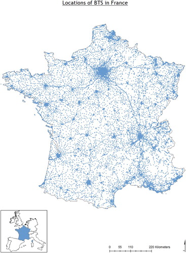
In this study, we use access to a CDR dataset by the telecom operator Orange and covering the French mainland. The dataset consists of the activities of ∼19 million subscribers during a period of 154 consecutive days in 2007 (May 13 to October 14) and gathers locational (the used cell-tower), temporal (time of action), and interactional information (who contacts whom) every time a call or text is initiated or received by the subscribers of the network. The spatial resolution of the dataset, therefore, is restricted to the spatial distribution of 17,385 cell-towers making up the Orange operational network in France. The locations of all cell-towers are known but their distribution in space is not uniform as can be observed in Figure A3 (in the Appendix). In general, higher densities of cell-towers can be found in more densely populated areas like cities or coastlines, as well as along transport axes. Lower densities of cell-towers are observed in more rural areas, as well as in mountain or natural areas. Summary metrics of the distributions of the circumference of the Voronoi polygons per Urban Area class (as defined by French National Statistics: INSEE) are displayed in Table A2 (See the Appendix). The differences in density of cell-towers (or thus the average spatial precision) are largest between major poles and suburban areas of major poles, with a mean Voronoi circumference of 7.6 km for centers of major poles and 25.4 km for surroundings of major poles. For medium poles and small poles differences between centers and surroundings become increasingly smaller, respectively 9.9 km (31.4–21.5) and 3.5 (34.9–31.4) km.

Figure 3. Correlations between cell-tower density (estimated by means of the Voronoi circumference of all cell-towers) and (a) average ME, (b) average CME All averages are calculated by the average value for all users having a detected ‘home’ at the concerned cell-tower. All parameter estimations for the linear regression are p < 0.05

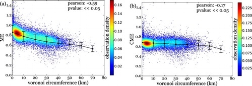
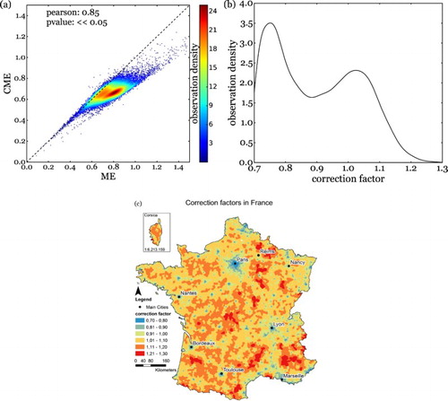
Figure 4. (a) Correlation between average ME and CME values, (b) The cumulative density function of the different correction factors (c_i) used for the calculation of CME (c) Spatial pattern of the correction factors (c_i)

In a first step of pre-processing, we limited the data to 44 consecutive days between September 1, 2007 and October 15, 2007. This period was chosen to avoid as much as possible the inclusion of holiday trips in the mobility pattern which typically occur during summer months, while still having a long enough observation period to capture daily routines. Previous studies indicate that a time period over one month is sufficient to capture habitual behavior (Schlich and Axhausen, 2003). Next, users from other providers or countries are omitted, as their registration on the network only happens occasionally as such no sound mobility patterns can be recorded. Finally, service numbers that do not belong to individuals as well as numbers that display machine-like activities, like highly frequent, highly repetitive or high-volume call patterns were omitted. The filtered, ultimately deployed dataset, stores a total of 3,926,725,446 location traces for 18,581,513 users of which 72.95 percent are derived from call and 27.05 percent from text actions.

To gain further insight in the differences between ME and CME at a nationwide scale, we investigate their relation with several socioeconomic and environmental variables in France obtained by census data and remote sensing. All socioeconomic variables were obtained from the French National Statistics office (INSEE) for the year 2007 and information for the environmental variables was retrieved from Corine Land Cover maps based on satellite images of 2006, both of which are freely available to the public. As census data is captured at the level of the administrative municipality, we change the spatial resolution of our investigation to the French municipality level when using them. We calculate value distributions for ME and CME per municipality by merging the observations of all cell-towers, and their related users, that are located in the same municipality. A list and description of the used socioeconomic and environmental variables is given in Table A1 (in the Appendix).

Methods

Mobility Entropy (ME) and Corrected Mobility Entropy (CME) indicators were calculated for all ∼18.5 million users in the French CDR dataset. In order to analyze their differences, spatial patterns, and relation with census data and remote sensing data, values for individual users were aggregated at the cell-tower level. Each of the 17,385 cell-towers in our dataset were attributed the average ME and CME values of all users that have a detected “home” at this cell-tower. To attribute cell-towers as “homes” to users in the CDR dataset we use the “time restraints” home-detection algorithm as described in Vanhoof et al. (2016, 2018). In this algorithm, we select, for each user, the cell-tower that had the highest amount of his/her activities during weekends and between 7 pm and 9 am on weekdays.

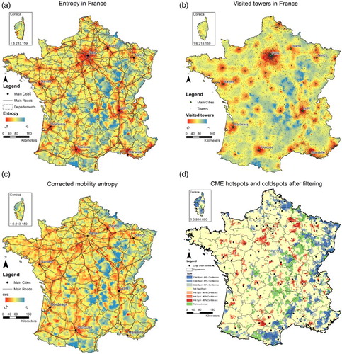
Spatial patterns of ME and CME values can consequently be analyzed based on the available geolocation of the cell-towers. To highlight spatial patterns, we used the Getis-Ord Gi* statistics as, for example, shown in Figure 5. This statistic reveals significant clusters of high (/low) values (hot- and cold-spots) as they are positioned in their wider environments. One remarkable observation when analyzing the Getis-Ord Gi* statistics of both ME and CME values was that multiple areas in France have statistically lower than expected values of both ME and CME (cold-spots). As most of these areas were remote or mountainous areas one could interpret human mobility to be different here. Another explanation, inspired by of the extreme low numbers of average visited cell-towers per user in these areas (See Figure 5b), is that individual movement is insufficiently observed in these areas (among others because of large Voronoi cells), resulting in abnormally low entropy values. In other words, the spatial resolution of the cell-tower network in these areas might not be sufficient to study the diversity of human mobility. As a consequence, we decided to filter out cell-towers where the average number of visited towers over the 1.5-month period is smaller than 10. The exact spatial pattern of this filtering is visible in Figure 5d. In total 814 out of 17,385 cell-towers were omitted; that is about 4.6 percent of the cell-towers in France.

Figure 5. Spatial patterns of (a) ME values (b) Number of visited towers per person over the 1.5-month period (c) CME values (d) Hotspots (red) and coldspots (blue) of CME values at different significance levels as calculated by the Getis-Ord Gi*-statistic Green areas accord to filtered-out cell-towers as described earlier

To obtain a clearer insight on the spatial patterns of ME and CME with respect to the urban system in France, we investigate their distributions when aggregated into the Urban Area classification as proposed by the French National Statistical Institute (INSEE). This classification is produced every five to ten years based on the identification of employment centers and their area of influence through commuting data.³ As such it goes beyond the typical physical borders defined by continuity of buildings often used in urban unit delineation and allows studying city organization and development based on the dynamic interactions between locations (Combes et al., 2016; Vanhoof et al., 2017).

As listed in Table 1, the Urban Area classification in France consists of nine classes, being distinguished mainly by the size of the employment center in the “central urban unit.” Major, medium, and small poles are employment centers offering respectively >10,000, between 5,000 and 10,000 and between 1,500 and 5,000 jobs. The surroundings of a pole are defined by identifying municipalities of which more than 40 percent of the working population commutes daily to this pole. Special cases are being recognized for municipalities that have several poles to commute to (multi-polarized municipalities) or municipalities that are not influenced by major, medium, or small poles (isolated municipalities). A spatial distribution of the Urban Areas in France is shown in the Appendix (See Figure A2). We calculate value distributions for ME and CME per Urban Areas by merging the observations of all cell-towers, and their related users that are located in the same urban area as defined by INSEE. Comparisons between distributions are done based on pairwise Wilcoxon Rank Sum test.

Table 1. Urban Areas as defined by INSEE, including the proportion of the number of municipalities and the number of cell-towers of Orange categorized in these classes

Urban Area Class	Description Urban Area Class	Municipalities (%)	Cell-towers (%)
111	Major Pole (more than 10.000 employments)	9	54
112	Surroundings of a major pole	34	18
211	Medium pole (5.000 to 10.000 employments)	1	3
212	Surroundings of a medium pole	2	1
221	Small pole (1.500 to 5.000 employments)	2	3
222	Surroundings of small pole	2	0.3
120	Multi-polarized, in a large urban area	11	5
300	Other multi-polarized municipalities	19	6
400	Isolated municipality outside influence	20	10

For the spatial pattern of this classification, see Appendix.

Ultimately, we investigate the relations between ME values, CME values, socioeconomic and environmental variables. Our goal here is to see how correcting mobility entropy influences the relation with socioeconomic and environmental variables, as well as to inform on the processes that lie behind the observed spatial patterns. In a first step, we calculate and plot the simple linear regression between ME values, CME values, and each socioeconomic or environmental variable pairwise. The simple linear regressions provide a direct insight in the relation between each pair of variables but do not allow for a proper comparison between independent variables with respect to their relevance in predicting ME or CME values. For this reason, we perform, in a second step, a multiple linear regression, using either ME or CME as dependent variable, and the normalized socioeconomic and environmental variables as independent variables. Note, we normalize all independent variables before creating the multiple regression models as it allows us to compare estimated regression coefficients (and their statistical significance) for each variable and hence to understand which variables have higher or lower predictive power in the respective models. Because of the considerable multicollinearity between several socioeconomic and environmental variables (for pairwise correlations between all socioeconomic and environmental variables (See Table A3), we perform our multivariate linear regression with interaction terms. The inclusion of interaction terms allows us to understand the degree to which the effect of an independent variable on the dependent variable varies as a function of a second independent variable, and, therefore, helps us better understand or, at least, hypothesize the processes at play.

Results

Correlating Mobility Entropy (ME), Corrected Mobility Entropy (CME), and Cell-Tower Density

Validation of both measures for human mobility is hard given that no ground truth is available, nor can possibly be collected in the future due to the scale of the dataset. Assessment of the proposed correction for mobility entropy, however, can be done by investigating the relation between ME, CME, and the cell-tower density. Remember that the main reason why we urged for a correction of the ME measure was because of its dependency on cell-tower density. This structural bias is apparent in Figure 3a where we find the Pearson correlation coefficient between ME and Voronoi circumference, our proxy for cell-tower density, to be as high as –0.59. Applying the proposed correction, or thus considering the CME values in Figure 3b, this correlation drops to –0.17. Although still showing a small negative trend, most probably because of the influence of the highest tower density areas (lowest Voronoi circumferences), it is fair to say the CME calculation largely diminishes the effect of cell-tower density, as was its initial goal. The result is promising: CME values are almost completely liberated from the structural bias of cell-tower density, rendering them more comparable between regions with differing densities of cell-towers.

To better understand the working of our proposed correction, we investigate the relationship between ME and CME for all cell-towers as given in Figure 4a. Cell-towers that have equal average ME and CME values are situated on the 1:1 line, but are few. Cell-towers that diverge from the 1:1 line are affected by the correction, with most of them experiencing a small decrease between ME and CME. This is also obvious from Figure 4b which shows the cumulative density distribution of the correction factors (c_i) as calculated by Equation 4. The bimodal distribution clearly indicates that most of the cell-towers have experienced a correction factor <1, with a peak around 0.78. Cell-towers that had an average correction factor >1 were observed less and, in general, corrected to a smaller degree as can be observed from the second peak around 1.03.

The spatial pattern of correction factors, as shown in Figure 4c clearly shows the first peak of (strongest) corrections (c_i around 0.78) to be located in the city centers throughout the country. This pattern is expected, as city centers typically have higher densities of cell-towers. Areas in which the correction factor augments the mobility entropy values most are rural and mountainous areas.

Spatial Patterns of (Corrected) Mobility Entropy in France

Above, we stated that higher densities of cell-towers, by definition of ME, result in higher values for n and lower values for p_i both combined resulting in higher values for ME. This argument is well illustrated by the clear accordance of the spatial patterns in Figure 5a and 5b showing, respectively, the average ME values and the average number of visited cell-towers (n) for users with presumed homes at each cell-tower. The spatial pattern shows a highly centered pattern with extensions that relate to, respectively, areas with high population densities and roads, once more supporting our argument that standard ME calculations are structurally biased.⁴.

On the contrary, the spatial pattern of CME values, as depicted in Figure 5c, renders a more homogenous spatial pattern that, although still highlighting cities and main roads, is less dominated by them. Interestingly, it seems as CME values, in comparison to ME values, are capable of differentiating smaller geographical regions. The most obvious example of this is the wider Paris region where despite having a rather constant density of cell-towers, spatial patterns of CME values are more complex compared to ME values.

Studying the hot- and cold-spots produced by the Getis-Ord Gi* statistic in Figure 5d, we observe that cold-spots are either located in border regions, near important passage roads, or in remote and mountainous areas that are close to filtered out areas. Possibly, mobility patterns are different in these areas, but more probably these cold-spots form an artifact of the data collection process. Similar to the filtered-out areas, the mountainous and remote areas close to them might suffer from limited spatial resolution of cell-towers resulting in insufficiently collected data to create representative mobility patterns. For border regions, even though average numbers of visited towers in these regions are higher and thus the spatial resolution of cell-towers can be deemed sufficient, it is highly plausible that movement patterns are collected only partially as we cannot observe cell phone activities outside the French territory.

Intriguingly, the hotspots of CME values are located just next to medium-sized and large-sized cities like Nantes, Rennes, Toulouse, and Lyon, but not in their city centers. Hypothetically, these clusters represent areas with high shares of commuters whom, besides commuting by car, also have a rather mobile lifestyle, as commuting solely would result in lower entropy values.⁵ The observation that such hotspots are found in the vicinity of almost all medium-sizes cities in France forms a strong suggestion towards the nation-wide comparability of the CME values.

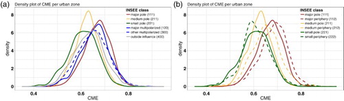
Investigating the distributions of ME and CME values when aggregated per Urban Area gives a clearer view regarding their relation with urban characteristics. Table 2 compares the distributions of ME and CME values per Urban Area by means of a Wilcoxon Rank Sum test and finds ME and CME value distributions to be statistically different in all urban areas except for the surroundings of small poles. Greatest differences are observable for the major urban pole class where ME values are clearly higher than CME values.

Table 2. Summary metrics of the distributions of ME and CME values and results from their pairwise Wilcoxon Rank Sum tests for different classes in the official Urban Area Classification

Urban Area class	Mean of ME values	Standard deviation of ME values	Mean of CME values	Standard deviation of CME values	Wilcoxon Rank Sum test (p-value)
Major pole	0.84	0.13	0.68	0.09	<0.01 (***)
Surrounding of major pole	0.76	0.09	0.69	0.08	<0.01 (***)
Medium pole	0.68	0.09	0.62	0.07	<0.01 (***)
Surrounding of medium pole	0.67	0.10	0.66	0.10	<0.01 (***)
Small pole	0.62	0.09	0.59	0.08	<0.01 (***)
Surrounding of small pole	0.63	0.09	0.63	0.09	0.6968 (Non-sign).
Multi-polarized in large urban area	0.69	0.09	0.65	0.08	<0.01 (***)
Other multi-polarized	0.67	0.10	0.66	0.09	<0.01 (***)
Outside urban influence	0.62	0.11	0.61	0.10	<0.01 (***)

Note: P-values are given on significance level <0.01 (***), <0.02 (**), <0.05(*).

Table 3 shows that distributions of CME values differ significantly between Urban Areas, making it a relevant delineation for our study. As can also be observed in Figure 6a, Urban Areas that develop around major employment centers depict (significantly) higher mobility diversity compared to all other Urban Areas. Multi-polarized municipalities, too, have high CME values, especially when situated near major poles. Municipalities outside the influence of poles have a rather high average CME value, but their wide distribution indicates the range of different situations that can be encountered in this category. The contrary can be said about the medium pole (and to a smaller extent, the major pole) class where a narrow distribution indicates similar observations of mobility diversity to be observed in different employment centers all over France.

Table 3. P-values of the Pairwise Wilcoxon Rank Sum tests between CME distributions of all different classes in the official Urban Area classification

Urban Area class	Major Pole	Surrounding of major pole	Medium Pole	Surrounding of medium pole	Small pole	Surrounding of small pole	Multipolarized in a large urban area	Other multi-polarized
Surrounding of major pole	<0.01 (***)
Medium pole	<0.01 (***)	<0.01 (***)
Surrounding of medium pole	<0.01 (***)	<0.01 (***)	<0.01 (***)
Small pole	<0.01 (***)	<0.01 (***)	<0.01 (***)	<0.01 (***)
Surroundings of small pole	0.02 (**)	<0.01 (***)	Non-sign.	<0.01 (***)	<0.01 (***)
Multi-polarized in a large urban area	<0.01 (***)	<0.01 (***)	<0.01 (***)	<0.01 (***)	<0.01 (***)	<0.01 (***)
Other multi-polarized	<0.01 (***)	<0.01 (***)	<0.01 (***)	Non-sign.	<0.01 (***)	<0.01 (***).	<0.01 (***)
Outside urban influence	<0.01 (***)	<0.01 (***)	Non-sign.	<0.01 (***)	<0.01 (***)	<0.01 (***)	<0.01 (***)	<0.01 (***)

Note: P-values are denoted by significance level <0.01 (***), <0.02 (**), <0.05(*).

Focusing on the relation between urban poles (employment centers) and their surroundings in Figure 6b, it is clear that surrounding areas of major and medium poles have higher CME values compared to their centers. Most remarkably, we find a clear decrease of CME values with size of the urban pole, both for the urban poles themselves and their surroundings. Bigger urban poles depict higher diversity of mobility both in their surrounding areas and centers, suggesting there is an interesting urban scaling law to be uncovered between both.

Relations between (Corrected) Mobility Entropy and Mobility-Related Variables

Besides investigating the spatial patterns, one outstanding question is how CME values relate to other variables, and to what degree our correction has altered relations compared to using ME values. Deploying simple linear regression models between ME, CME, and several socioeconomic or environmental variables in France offer some initial insights, especially since comparing the relation between ME and variable x to the relation between CME and the same variable x, allows us to highlight the difference between ME and CME introduced by our correction. Figure 7 and Table 4 show the simple linear regressions between ME, CME, and a selection of variables such as income, share of public transportation use, and land use. Table A1 (in the Appendix) gathers the results of all simple linear regressions.

Figure 7. Linear regression between collected variables related to mobility and ME or CME values Densities of observation points in the plot are color-coded and base on the absolute numbers of observations in the plot area. Adjusted R² measures are given, as well as p-values, and estimates for intercept and slope of the regression. Values for CME and ME are calculated for all cell-towers in France as the average value of all users that have a ‘home’ at these cell-towers. Values for median income, trips by car or public transport and employment in residence of commune are based on French census data. Shares of land-use are based on Corine data

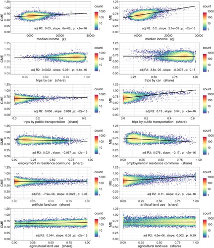
Table 4. Regression coefficient estimates for single linear regression models predicting ME or CME values

Variable	Description	Correlation with CME	Correlation with ME
Median income	The median income per household member	0.000006 0.030 (***)	0.000021 0.19 (***)
Car share	The share of trips made by car	0.031 0.0022 (***)	–0.0073 0.000035 (0.15)
Public transportation share	The share of trips made by public transportation	0.068 0.0059 (***)	0.54 0.12 (***)
Employment in municipality	The share of people working in their municipality of residence	–0.067 0.020 (***)	–0.17 0.076 (***)
Artificial land use	The share of artificial land use in a municipality	0.0023 –0.00000077 (0.37)	0.2 0.10 (***)
Agricultural land use	The share of agricultural land use in a municipality	0.05 0.044 (***)	0.02 0.0000043 (0.28)

Note: The regression coefficient (top), adjusted R² measures (bottom left), and p-values (bottom right) on significance level <0.01 (***), <0.02 (**), <0.05(*), or exact p-value, or exact p-value are given.

In general, simple linear regressions have very little predictive power (low adjusted R²-values) and using CME instead of ME values does not implicate radical shifts in observed (simple) regression coefficients. Relations do tend to be less pronounced when using CME, which is not really surprising given the smoothing effect of the correction factor. What is remarkable though is that by using CME instead of ME, three relations shift significance (See Table 4). When correcting ME to CME, the share of artificial land use in a municipality becomes insignificant to explain mobility diversity. This is not really surprising as the share of artificial land use highly coincides with cell-tower density, which was the focus of our correction. Correcting mobility entropy for cell-tower density, therefore, also renders the relation between artificial land use and mobility entropy insignificant. The opposite is observed for the share of agricultural land use and the share of car as a transport mode which both become significant when correcting to CME. These shifts in significance coincide well with previous findings. Here too, these shifts imply CME values to be higher in areas with higher agricultural shares (like rural areas, but also certain suburban areas, especially around smaller city centers) whereas based on ME values one would expect mobility diversity to be higher in areas with higher artificial land use (like larger city centers). With this pattern in mind, it is extremely interesting to notice that CME values unveil the role of car use as transport mode as a possible explanatory factor for mobility diversity whereas ME values did not.

The insights that can be obtained from simple regressions are rather limited, especially because of the small predictive power that has been obtained by these models. For this reason, we deploy two multiple regression models incorporating all independent variables and their interaction terms in order to predict either ME or CME values. Doing so allows us to gain an insight into which variables are more powerful in predicting nationwide value distributions for ME and CME, as this could help to improve predictions over simple regression models. Table 5 shows all statistically significant parameters with an estimated regression coefficient larger than 0.1 (or for negative coefficients smaller than –0.1) for the two multiple regression models (one for ME, the other for CME values). We use the normalized values for all independent variables meaning that we can compare the magnitude of the estimated regression coefficients between independent variables. Full information of both multiple regression models is given in Tables A4 and A5 (in the Appendix).

Table 5. Regression coefficient estimates for a selected set of independent variables for two multiple linear regression models predicting either ME or CME values

Multiple linear regression for dependent variable: ME (R^2 = 0.404, R^2-adj. = 0.401)				Multiple linear regression for dependent variable: CME (R^2 = 0.189, R^2-adj. = 0.185)
	Estimate	t-statistic	Pr(>|t|)		Estimate	t-statistic	Pr(>|t|)
Median income	0.23	34.09	0.000(***)	Land use artificial	–0.20	–5.98	0.000(***)
Public transport (share)	0.20	20.08	0.000(***)	Active population	0.20	30.09	0.000(***)
City distance	–0.20	–31.40	0.000(***)	Mean elevation	–0.16	–14.55	0.000(***)
Active population	0.17	29.86	0.000(***)	City distance	–0.13	–17.48	0.000(***)
Mean elevation	–0.14	–15.36	0.000(***)	Median income	0.12	15.53	0.000(***)
Land use forest	–0.11	–2.42	0.015(**)	LU artificial:Car (share)	0.12	2.97	0.003(***)
LU forest:City distance	0.11	2.33	0.020(**)	Employed in municipality	0.12	12.11	0.000(***)
LU agriculture:City distance	0.11	2.25	0.025(*)	LU forest:Car (share)	0.16	2.49	0.013(**)
LU forest:Car (share)	0.11	2.06	0.040(*)	LU_agriculture:Car (share)	0.15	2.21	0.027(*)

Note: For both models adjusted R² measures, regression coefficients and related p-values (rounded at 3 decimals) based on the t-statistic are given with significance levels <0.01 (***), <0.02 (**), and <0.05(*). Estimates were selected on (i) having a p-value significant at, at least, 0.05 level and (ii) having a coefficient estimate with an absolute value higher than 0.1. Estimates are organized by significance level and sorted by absolute value of the coefficient estimate.

Investigating both multiple regression models, as partially displayed in Table 5, we can see that the predictive power of the ME model is quite a lot higher than the CME model (R² of 0.40 versus 0.18), even though the same independent variables were used. Investigating the most significant explanatory variables and their predictive force we find the ME model to have a set of significant and strongly explanatory variables, like distance to a large city, median income and share of public transport as transport mode, that, interpretatively, align well with the definitions of larger city centers. A finding that, given the nature of the ME calculations and the cell-tower density bias, could be expected. Additionally, there is a second set of variables that are both less explanatory and less significant and seem to deal with non-urban environments. Here a focus lies on municipalities with higher shares of forest, and mainly through interaction terms of remoteness. This too is not entirely unexpected in relation to the cell-tower density bias for ME values as remote forest areas typically relate to low-density cell-tower areas.

The multiple regression model predicting CME values is rather different. Although geographical elements (distance to large city, elevation) remain more or less similar, the median income factor now seems to share its predictive force with the share of workforce employed in the municipality and also the demographic aspect of active workers in the population gains importance in the model. More remarkable, however, is that the share of public transport as travel mode has become insignificant and there is the appearance of a strong and significant factor in the form of the share of artificial land use. The role of the artificial land use share is puzzling, as it has a large negative regression coefficient, which is not entirely expected given the non-existent relation in the simple linear regression discussed before. Its role, however, is partly balanced out by a strong positive interaction effect between artificial land use and the share of the car as transport mode. An interesting point is that the same interaction effects for the other available land-use classes also have a prominent role in the model, rendering the combination of car and land use one of the cornerstones for the interpretation of nationwide CME patterns.

Reflecting on the lower predictive power of the model for CME (R² of 0.18) compared to the model for ME (R² of 0.40), one could argue that its focus on typically (large) urban characteristics probably boosts its predictive force given that a large share of French municipalities are classified under the influence of major poles or within a large urbanized area (around 65 percent as can be derived from Table 1). The CME model probably is not capable of mining this quick win in predictive force, making it less efficient in pure prediction. This, however, does not mean the CME model is less useful for research. After all, the model indicates that some general tendencies can be derived but that local situations are probably far more complex and in need of further in-depth study.

Discussion

Throughout our investigation we argued that the traditional indicator used to describe individual movement diversity from movement patterns, the mobility entropy, is dependent on the amount of possible observation points. This is problematic given that several new technologies allow us to collect data on human movement for large-scale populations, but do not possess observation points that are evenly distributed over the territory. Differing densities of observation points, like cell-towers for mobile phone data or check-in places for location-based services, therefore introduce a structural bias in the calculation of mobility entropy, obscuring our insights and interpretations. Investigations on small-scale areas with more or less constant densities of observation points will be less prone to this bias but if we want to take full advantage of large-scale geographical datasets, the bias needs to be accounted for.

On a more general note, we reckon that even though current data coverage might be large-scale, this doesn’t automatically imply that our analytics are objective at such a large scale. Biases occur in different ways and at different scales as they might be due to, among other factors, changing context and user groups, non-objective data collection methods, or even unthoughtful methodology. As a consequence, critical evaluation becomes crucial in the largely empirical research domains that are emerging around large-scale data captured by new information technologies.

The main problem, in this perspective, remains the absence of proper validation data that, even if only to a small degree, could match the extent and diversity of the newly gathered data sources. Obviously, this absence strongly complicates validation of current research practices. It also frustrates efforts to challenge existing practices since neither the claimer nor the challenger has solid ground to prove its “trustworthiness.” The situation of this study is similar. Through publications (Pappalardo et al., 2016; Song, Qu, et al., 2010) and implementation in software packages like bandicoot.py (de Montjoye et al., 2016), the use of the mobility entropy indicator is slowly becoming institutionalized even though no validation efforts have yet been published and thus little discussion on its trustworthiness has yet been conducted.

In this paper, we challenge the use of the standard mobility entropy for comparison between large-scale regions. As we are the first to explicitly investigate the spatial pattern of mobility entropy at nation-wide scale, we revealed its sensitivity to changing densities of observations points and showed how this troubles interpretation in relation to, for example, urban areas or census data. We argued that a correction is necessary and proposed Corrected Mobility Entropy (CME) as a solution. Even though it remains difficult to validate our proposed correction and, to a lesser extent, the parameter choices we make, we clearly documented our train of thought and turned to a detailed investigation of the case of mobile phone data in France.

One outstanding question is how our proposed correction would translate to other geo-located large datasets like for instance those collected from LBS or OSN. The underlying assumption when constructing the correction factor for mobile phone data is that their use (for calling/texting) is independent from the (passive) location recording. This assumption does not hold for location based social media or online social networks where location recording is an active act embedded in the mediated use of the service. As such, for these applications the heterogeneous possibility of being detected in a location is not only given by a spatial, infrastructural element (the density of possible check-in locations in an area) but also, and possibly even more so, by the mediation of these locations within the application (the “attractivity” of sharing this location within the context of the application). This extra layer of heterogeneity most probably needs to be accounted for when constructing a correction factor for such applications.

For the case of mobile phone data in France, our findings show that the proposed Corrected Mobility Entropy (CME) is less correlated to cell-tower density compared to standard Mobility Entropy (ME) values, hence reducing the bias when comparing CME values for regions with different cell-tower densities. Except for some regions, which we identify as border regions or regions with limited coverage, CME values across France are interpretable as they form a coherent spatial pattern (See Figure 5c), have significant relationships with other mobility related variables derived from census or satellite images (See Tables 4 and 5 and Figure 7) and depict significantly different distributions for different Urban Areas (See Figure 6 and Table 3).

Figure 6. Density plot of CME values per class in the official Urban Area classification. For different Urban Areas (a) and focus on the three main urban classes and their sub-urban areas (b) Values are calculated for all cell-towers in France as the average of all users that have a ‘home’ at these cell-towers

Interestingly, correcting ME to CME does not result in fundamentally changing relations with socioeconomic, mobility-related indicators provided by census as expressed by the simple linear regressions in Table 4 and Figure 7. This is true for all investigated census indicators except for one: the share of car use during trips. In this case, the relation with ME is insignificant, but the relation with CME becomes significant. Given the important role of cars in terms of accessibility and individual mobility, this is an important finding that seems to endorse our argument for CME.

Despite only a minor shift in the relation with socioeconomic variables, correcting ME for cell-tower density has a profound effect on the spatial pattern of observed mobility entropy as can be seen by comparing Figure 5a and 5c and as has been proven statistically at the Urban Area level in Table 2. The relation between CME values and the French urban system becomes clearer when investigating the distributions of CME values in different Urban Areas as was done in Figure 6. To our surprise, using the Urban Area classification proposed by the French National Statistics Office rendered significantly different distributions of observed degrees of mobility diversity for (almost) all urban areas (See Table 3). We find distributions of CME values to be significantly larger in surrounding areas compared to their related urban poles. Additionally, we find mobility diversity based in both urban and suburban regions to decrease considerably with lowering urban center sizes (See Figure 6b), suggesting the existence of a scaling law for mobility diversity in France.

Trying to interpret the spatial patterns of ME and CME values based on their relationship with both socioeconomic and environmental variables confirmed the idea that CME appropriate suburban zones as the locations where mobility diversity is highest, compared to city centers for ME. The simple regression models using land use as independent variable in Table 4 and Figure 7 already hinted towards such an interpretation. They showed CME to have a significant relation with share of agricultural land use but not with the share of artificial land use in a municipality, whereas the opposite was found for ME values. The results from two multiple regression models, as given in Table 5, allow for a more elaborate interpretation. The multiple regression model to predict ME values can be interpreted as operating in an urban-remote dichotomy, focusing mostly on characteristics both geographical (city distance, elevation, land use) and economical (median income, share of active population, and share of public transport as transport mode) that allows for the distinguishing of large city centers. In contrast, the multiple regression model to predict CME values, although less explanatory in its whole, does not focus on this urban–remote dichotomy. Instead, it unveils a more complex process that encompasses interactions between employment centers, distances to cities, demographics, incomes, land use, and the role of the car as its main explanatory dimensions. According to the multiple regression models, higher (corrected) mobility entropies can be expected in areas that are economically active (higher active population, higher median income, higher employment within the municipality), where the share of car use for trips is higher and independent from which land use is predominant (although interaction terms strongly suggest there to be different regimes for different land use mixes), and that are situated closer to large cities, typically on lower elevations, and with a smaller share of artificial land use. It is reassuring, that such a description matches well with what can be expected from suburban areas, especially around medium and large cities, which are also the locations of hotspots for CME values as can be seen in Figure 5d.

All of these findings suggest a strong link between individual mobility diversity and the urban system, which opens up exciting research opportunities in urban geography and planning, mobility and transport modelling, or even in official statistics. Given that monitoring of individual mobility diversity for nationwide populations can be done rather easily by CDR data, the use of CME values presents itself as a prerequisite step to understand, monitor, and evaluate changes in the dynamics between human mobility and the urban system.

Conclusion

In this paper, we focused on the derivation of the so-called Mobility Entropy (ME) from mobile phone records as an indicator of the diversity of individual movement. Being the first to look into nationwide, spatial patterns of mobility entropy, we raised the issue that standard ME calculations depict a structural dependency on cell-tower density, rendering comparison of ME values between regions biased. As a solution, we proposed a correction in the form of the Corrected Mobility Entropy (CME).

We applied our solution to a French CDR dataset calculating CME values for ∼18.5 million users. Our results show the corrected mobility entropy (CME) to be less correlated to cell-tower density (r = –0.17) and to render a different, more detailed spatial pattern compared to the traditional mobility entropy (ME) which has a strong correlation with cell-tower density (r = –0.59) and a clear bias towards areas with high cell-tower densities like cities or major roads.

To better understand the spatial patterns of CME values in France, we investigated the relationship with several socioeconomic and land use indicators from census or satellite image data. By means of both single and multiple linear regressions we show the diversity of individual movement to be related to factors like income, the share of car use in trips, employment in the municipality of residence, land use, and the distance to large cities. The obtained regression models reveal several significant variables, but are limited in predictive power, indicating the more complex and, probably, local nature of relations left to explore. Compared to the same regressions performed on traditional ME values, we find using CME installs a significant relation with use of cars with a strong suggestion towards different regimes for different land use classes.

Focusing on the regional patterns of CME values, we found significant differences between distributions of CME values for different Urban Areas as defined by the French National Statistical Institute (INSEE). Our main findings show diversity of mobility to be highest in suburban regions, with distributions of CME values being significantly larger in suburban regions compared to their related urban centers. Additionally, we find mobility diversity in both urban and suburban regions to decrease considerably with lowering urban center sizes, suggesting an urban scaling law for mobility diversity in France.

All our findings suggest our proposed correction of mobility entropy (CME) to result in a more reliable indicator when it comes to comparing the diversity of human movement between large-scale regions based on mobile phone data. As our analysis allows more correct describing, understanding, and delineating of regions or urban areas with respect to individual mobility, we believe our findings to be relevant for planning and policy, especially from the perspective of urban development, and to have clear applications in official statistics, urban planning, and mobility research.

The underlying research materials for this article can be accessed at https://doi.org/10.17634/154300-80. Some data supporting this article is not openly available because of confidentiality considerations. Please contact Newcastle Research Data Service at [email protected] for further information..

Acknowledgments

The authors wish to thank Orange Labs, especially the SENSE department, for making the data available. We also like to acknowledge the Erasmus+ Traineeship program. Also, we would like to thank Gerard (Gerry) Wilkinson for his help in preparing the manuscript. Finally, we dedicate this paper to Rein Ahas, a dear friend and a valued colleague. We will miss him and his kind advice, offered on this paper and on other research. He was a mentor and a leader in the field whose loss will be felt by many.

Disclosure Statement

No potential conflict of interest was reported by the authors.

Notes on Contributors

Maarten Vanhoof is a PhD candidate at the Open Lab in Newcastle University and Orange Labs in Paris. His research focuses on the use of mobile phone data for geographical research and official statistics.

Willem Schoors received his MSc degree in Geography (GIS and spatial modelling) from the Katholieke Universiteit Leuven, Belgium. He is currently employed at Geo Solutions, where he focuses on geospatial application development.

Anton Van Rompaey is a professor in Geography at KU Leuven, Belgium.

Thomas Ploetz is an associate professor at the School of Interactive Computing, Georgia Tech, USA.

Zbigniew Smoreda is a sociologist and researcher at Orange Labs’ Sociology and Economics of Networks and Services (SENSE) Department.

ORCID

Maarten Vanhoof http://orcid.org/0000-0001-9591-024X

Willem Schoors http://orcid.org/0000-0001-6383-844X

Anton Van Rompaey http://orcid.org/0000-0001-5435-6887

Thomas Ploetz http://orcid.org/0000-0002-1243-7563

Zbigniew Smoreda http://orcid.org/0000-0002-4047-7597

Additional information

Funding

Maarten Vanhoof is funded by the EPSRC Center for Doctoral Training in Digital Civics [grant no. EP/L016176/1].

Notes

1 In the case of CDR data, observation points are equal o cell-towers, which is the spatial resolution in which the data is observed.

2 For an extensive literature review on the different applications of CDR data in research, see Blondel, Decuyper, and Krings, 2015.

3 The 2010 Urban Area classification is based on data collected between 2006 and 2010 in the national census survey.

4 Rememer that we want our ME measure to express the diversity of movement, not the absolute number of visited towers. A direct relation between both indicates an (unwanted) dependency induced by higher chances of visiting more cell-towers in areas with high cell-tower density, rather than an objective measurement of movement diversity.

5 Given the definition, movement patterns that are often repeated, like commuting back and forth between work and home, contribute little to the entropy, resulting in low entropy values. They are the opposite of a diverse movement pattern.

Appendix

Figure A1. Sensitivity of correlations between cell-tower density and average CME values of all cell-towers calculated with scaling range (a–b) between (a) 0.5–1.5, (b) 0.6–1.4, (c) 0.8–1.2, (d) 0.9–1.1 Cell-tower densities are estimated by means of the Voronoi circumference. All averages are calculated by the average value for all users having a detected ‘home’ at the concerned cell-tower. All parameter estimations for the linear regression are p < 0.05

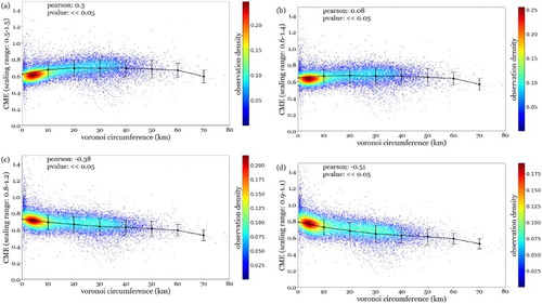
Figure A2. Spatial distribution of the Urban Area Classes. Source: Combes et al., 2017, based on Brutel and Levy, 2011

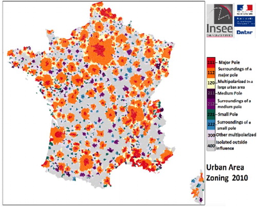
Figure A3. Spatial distribution of Orange cell-towers in France

Table A1. Correlation between collected variables related to mobility, ME and CME values

Variable	Description	Correlation with ME	Correlation with CME
Median income	The median income per household member	0.19 (***)	0.030 (***)
Active population	The share of municipality population between 15 and 65 years old	0.095 (***)	0.0095 (***)
Working population	The employed share of the active population	0.06 (***)	0.011 (***)
Commuting distance	The median commuting distance for a municipality^1	0.097 (***)	0.014 (***)
Car share	The share of trips made by car	0.000035 (0.15)	0.0022 (***)
Public transportation share	The share of trips made by public transportation	0.12 (***)	0.0059 (***)
Car ownership	The average number of cars owned per household	0.0011 (***)	0.011 (***)
Employment in municipality	The share of people working in their municipality of residence	0.075 (***)	0.020 (***)
Mean elevation	The mean elevation of the municipality^2	0.042 (***)	0.036 (***)
Artificial land use	The share of artificial land use in a municipality^3	0.10 (***)	–0.00000077 (0.37)
Agricultural land use	The share of agricultural land use in a municipality^3	0.0000043 (0.28)	0.044 (***)
Natural land use	The share of forest in a municipality^3	0.040 (***)	0.051 (***)
Road distance	Average distance in the municipality to nearest major road^4	0.019 (***)	0.0019 (***)
City distance	Average distance in the municipality to nearest city with > 20,000 inhabitants	0.14 (***)	0.027 (***)
Station distance	Average distance in the municipality to nearest train station	0.033 (***)	0.0059 (***)

Adjusted R² measures are given, as well as p-values on significance level <0.01 (***), <0.02 (**), <0.05(*), or the exact p-value. Superscripts are: 1: Based on CDR data, 2: Based on SRTM data, 3: Based on Corine data, 4: Major roads equal the regional road network.

Table A2. Summary metrics for the distributions of circumferences of the Voronoi polygons for all cell-towers in different classes in the official Urban Area Classification

	Circumference of Voronoi Polygons
Urban Area class	Mean	Standard deviation	0% quantile (minimum)	25% quantile	50% quantile (median)	75% quantile	100% quantile (maximum)
Major pole	7.6	6.8	0.1	2.9	5.4	10.3	72.0
Surrounding of major pole	25.4	9.3	1.9	18.3	25.0	31.6	67.8
Medium pole	21.0	9.6	0.2	13.2	21.5	27.9	48.0
Surrounding of medium pole	32.2	8.3	14.3	26.4	31.4	38.0	51.6
Small pole	31.3	11.6	4.4	24.3	31.4	38.8	74.7
Surrounding of small pole	35.7	7.8	16.8	29.9	34.9	41.7	50.6
Multi-polarized in a large urban area	29.0	8.8	5.5	22.8	28.7	34.7	62.2
Other multi-polarized	33.5	8.8	6.1	27.9	33.4	39.2	71.3
Outside urban influence	36.4	11.3	3.6	29.2	36.5	43.6	79.0

Note: All metrics are in km.

Table A3. Pairwise Correlation coefficients between all mobility related variables used in the analysis

	Employment municipality	Car ownership	Public transport share	Car share	Commute distance	Active pop.	Working pop.	Median income	Station distance	City distance	Road distance	Natural land use	Agriculture land use	Artificial land use
Mean elevation	0.26	–0.03	–0.10	–0.11	0.19	0.08	–0.06	–0.05	0.10	0.27	0.15	0.58	–0.45	-0.15
Artificial land use	0.01	–0.38	0.56	–0.30	–0.32	–0.15	0.15	0.29	–0.22	–0.28	–0.25	–0.18	–0.38
Agricultural land use	–0.16	0.24	–0.26	0.19	0.04	0.19	–0.03	–0.17	–0.05	–0.04	0.01	–0.83
Natural land use	0.16	–0.03	–0.06	–0.02	0.15	–0.12	–0.05	0.01	0.18	0.21	0.14
Road distance	0.07	0.07	–0.12	–0.01	0.19	0.00	–0.12	–0.15	0.11	0.14
City distance	0.35	–0.06	–0.14	–0.17	0.49	–0.10	–0.32	–0.28	0.26
Station distance	0.23	–0.03	–0.19	–0.02	0.23	–0.13	–0.19	–0.20
Median income	–0.32	0.10	0.33	0.03	–0.27	0.27	0.39
Working population	–0.42	0.15	0.23	0.14	–0.28	0.21
Active population	–0.28	0.26	0.02	0.13	–0.05
Commuting distance	0.27	–0.03	–0.14	–0.13
Car share	–0.48	0.46	–0.48
Public transp. share	–0.13	–0.27
Car ownership	–0.39

Note: All correlations have p-values <0.01.

Table A4. Regression coefficient estimates for multiple linear regression model predicting the ME values

Variable or Interaction term	Estimate	Pr(>|t|)
Intercept	–0.037	0.000
Mean Elevation	–0.143	0.000
LU artificial	0.034	0.236
LU agricultural	–0.030	0.524
LU forest	–0.109	0.015
Road Distance	–0.012	0.032
City Distance	–0.201	0.000
Station Distance	–0.011	0.214
Median Income	0.226	0.000
Active population	0.040	0.000
Working population	0.170	0.000
Commuting Distance	–0.067	0.000
Car share	0.053	0.000
Public Trans. share	0.205	0.000
Car ownership	0.035	0.000
Employment in Mun.	0.042	0.000
Mean Elevation:LU artificial	–0.002	0.959
Mean Elevation:LU agricultural	–0.007	0.900
Mean Elevation:LU forest	–0.014	0.785
Mean Elevation:Road Distance	0.029	0.000
Mean Elevation:City Distance	0.035	0.000
Mean Elevation:Station Distance	–0.008	0.165
Mean Elevation:Median Income	–0.032	0.000
Mean Elevation:Active population	0.018	0.005
Mean Elevation:Working population	0.028	0.000
Mean Elevation:Commuting Distance	0.023	0.000
Mean Elevation:Car share	–0.011	0.155
Mean Elevation:Public Trans. share	–0.002	0.835
Mean Elevation:Car ownership	–0.012	0.095
Mean Elevation:Employment in Mun.	0.031	0.000
LU artificial:LU agricultural	0.005	0.545
LU artificial:LU forest	–0.008	0.480
LU artificial:Road Distance	–0.036	0.148
LU artificial:City Distance	0.032	0.239
LU artificial:Station Distance	0.037	0.293
LU artificial:Median Income	0.038	0.049
LU artificial:Active population	–0.011	0.643
LU artificial:Working population	0.007	0.788
LU artificial:Commuting Distance	0.028	0.245
LU artificial:Car share	0.082	0.017
LU artificial:Public Trans. share	0.046	0.081
LU artificial:Car ownership	0.034	0.248
LU artificial:Employment in Mun.	–0.028	0.337
LU agricultural:LU forest	–0.022	0.001
LU agricultural:Road Distance	–0.003	0.945
LU agricultural:City Distance	0.108	0.025
LU agricultural:Station Distance	0.080	0.177
LU agricultural:Median Income	0.072	0.037
LU agricultural:Active population	–0.059	0.177
LU agricultural:Working population	0.047	0.271
LU agricultural:Commuting Distance	0.076	0.069
LU agricultural:Car share	0.111	0.058
LU agricultural:Public Trans. share	0.009	0.845
LU agricultural:Car ownership	0.015	0.770
LU agricultural:Employment in Mun.	–0.072	0.165
LU forest:Road Distance	–0.033	0.406
LU forest:City Distance	0.105	0.020
LU forest:Station Distance	0.093	0.093
LU forest:Median Income	0.069	0.037
LU forest:Active population	–0.038	0.362
LU forest:Working population	0.015	0.713
LU forest:Commuting Distance	0.068	0.085
LU forest:Car share	0.114	0.040
LU forest:Public Trans. share	0.006	0.901
LU forest:Car ownership	0.014	0.765
LU forest:Employment in Mun.	–0.059	0.224
Road Distance:City Distance	0.002	0.700
Road Distance:Station Distance	0.000	0.975
Road Distance:Median Income	0.008	0.204
Road Distance:Active population	–0.013	0.018
Road Distance:Working population	–0.009	0.090
Road Distance:Commuting Distance	–0.016	0.007
Road Distance:Car share	0.005	0.436
Road Distance:Public Trans. share	–0.024	0.002
Road Distance:Car ownership	–0.017	0.002
Road Distance:Employment in Mun.	–0.004	0.589
City Distance:Station Distance	–0.016	0.000
City Distance:Median Income	–0.018	0.010
City Distance:Active population	0.000	0.942
City Distance:Working population	–0.038	0.000
City Distance:Commuting Distance	–0.048	0.000
City Distance:Car share	–0.023	0.003
City Distance:Public Trans. share	0.061	0.000
City Distance:Car ownership	–0.006	0.373
City Distance:Employment in Mun.	–0.011	0.129
Station Distance:Median Income	–0.024	0.001
Station Distance:Active population	0.004	0.443
Station Distance:Working population	–0.009	0.097
Station Distance:Commuting Distance	–0.008	0.123
Station Distance:Car share	0.020	0.005
Station Distance:Public Trans. share	–0.009	0.470
Station Distance:Car ownership	–0.006	0.404
Station Distance:Employment in Mun.	–0.008	0.138
Median Income:Active population	0.027	0.000
Median Income:Working population	–0.019	0.001
Median Income:Commuting Distance	–0.004	0.608
Median Income:Car share	0.002	0.830
Median Income:Public Trans. share	0.023	0.001
Median Income:Car ownership	0.052	0.000
Median Income:Employment in Mun.	0.023	0.004
Active population:Working population	0.003	0.544
Active population:Commuting Distance	–0.018	0.002
Active population:Car share	0.012	0.083
Active population:Public Trans. share	0.030	0.000
Active population:Car ownership	–0.011	0.062
Active population:Employment in Mun.	0.018	0.009
Working population:Commuting Distance	0.011	0.066
Working population:Car share	0.014	0.042
Working population:Public Trans. share	–0.008	0.327
Working population:Car ownership	–0.024	0.000
Working population:Employment in Mun.	–0.056	0.000
Commuting Distance:Car share	–0.019	0.006
Commuting Distance:Public Trans. share	–0.050	0.000
Commuting Distance:Car ownership	0.001	0.916
Commuting Distance:Employment in Mun.	–0.016	0.011
Car share:Public Trans. share	0.062	0.000
Car share:Car ownership	0.008	0.162
Car share:Employment in Mun.	0.021	0.001
Public Trans. share:Car ownership	–0.031	0.000
Public Trans. share:Employment in Mun.	0.036	0.000
Car ownership:Employment in Mun.	0.056	0.000

Note: P-values are calculated based on a t-statistic.

Table A5. Regression coefficient estimates for multiple linear regression model predicting the CME values

Variable or Interaction term	Estimate	Pr(>|t|)
Intercept	–0.02	0.045
Mean Elevation	–0.16	0.000
LU artificial	–0.20	0.000
LU agricultural	0.09	0.109
LU forest	–0.05	0.326
Road Distance	–0.02	0.000
City Distance	–0.13	0.000
Station Distance	0.01	0.513
Median Income	0.12	0.000
Active population	–0.02	0.005
Working population	0.20	0.000
Commuting Distance	–0.04	0.000
Car share	0.05	0.000
Public Trans. share	0.10	0.000
Car ownership	0.04	0.000
Employment in Mun.	0.12	0.000
Mean Elevation:LU artificial	–0.03	0.470
Mean Elevation:LU agricultural	–0.12	0.053
Mean Elevation:LU forest	–0.12	0.035
Mean Elevation:Road Distance	0.02	0.001
Mean Elevation:City Distance	0.05	0.000
Mean Elevation:Station Distance	–0.01	0.224
Mean Elevation:Median Income	–0.02	0.080
Mean Elevation:Active population	0.03	0.000
Mean Elevation:Working population	0.01	0.149
Mean Elevation:Commuting Distance	0.02	0.001
Mean Elevation:Car share	–0.01	0.253
Mean Elevation:Public Trans. share	0.00	0.821
Mean Elevation:Car ownership	–0.02	0.015
Mean Elevation:Employment in Mun.	0.05	0.000
LU artificial:LU agricultural	–0.06	0.000
LU artificial:LU forest	–0.07	0.000
LU artificial:Road Distance	–0.07	0.014
LU artificial:City Distance	–0.01	0.846
LU artificial:Station Distance	0.03	0.491
LU artificial:Median Income	0.04	0.085
LU artificial:Active population	–0.01	0.654
LU artificial:Working population	0.05	0.087
LU artificial:Commuting Distance	0.05	0.076
LU artificial:Car share	0.12	0.003
LU artificial:Public Trans. share	0.04	0.194
LU artificial:Car ownership	0.04	0.244
LU artificial:Employment in Mun.	0.05	0.156
LU agricultural:LU forest	0.00	0.546
LU agricultural:Road Distance	–0.03	0.498
LU agricultural:City Distance	0.08	0.138
LU agricultural:Station Distance	0.09	0.171
LU agricultural:Median Income	0.06	0.110
LU agricultural:Active population	–0.06	0.273
LU agricultural:Working population	0.09	0.069
LU agricultural:Commuting Distance	0.08	0.091
LU agricultural:Car share	0.15	0.027
LU agricultural:Public Trans. share	0.00	0.934
LU agricultural:Car ownership	0.01	0.897
LU agricultural:Employment in Mun.	0.05	0.440
LU forest:Road Distance	–0.05	0.237
LU forest:City Distance	0.07	0.209
LU forest:Station Distance	0.09	0.172
LU forest:Median Income	0.05	0.236
LU forest:Active population	–0.03	0.572
LU forest:Working population	0.06	0.184
LU forest:Commuting Distance	0.08	0.070
LU forest:Car share	0.16	0.013
LU forest:Public Trans. share	0.00	0.971
LU forest:Car ownership	0.01	0.817
LU forest:Employment in Mun.	0.02	0.703
Road Distance:City Distance	0.00	0.621
Road Distance:Station Distance	0.01	0.329
Road Distance:Median Income	0.02	0.009
Road Distance:Active population	–0.02	0.004
Road Distance:Working population	–0.02	0.001
Road Distance:Commuting Distance	–0.01	0.050
Road Distance:Car share	0.00	0.632
Road Distance:Public Trans. share	–0.01	0.134
Road Distance:Car ownership	–0.02	0.001
Road Distance:Employment in Mun.	0.00	0.793
City Distance:Station Distance	–0.01	0.011
City Distance:Median Income	–0.03	0.002
City Distance:Active population	–0.01	0.199
City Distance:Working population	–0.06	0.000
City Distance:Commuting Distance	–0.06	0.000
City Distance:Car share	–0.02	0.006
City Distance:Public Trans. share	0.06	0.000
City Distance:Car ownership	–0.01	0.510
City Distance:Employment in Mun.	–0.02	0.029
Station Distance:Median Income	–0.01	0.384
Station Distance:Active population	0.00	0.733
Station Distance:Working population	–0.01	0.071
Station Distance:Commuting Distance	–0.01	0.037
Station Distance:Car share	0.01	0.171
Station Distance:Public Trans. share	0.01	0.557
Station Distance:Car ownership	–0.01	0.289
Station Distance:Employment in Mun.	–0.01	0.070
Median Income:Active population	0.03	0.000
Median Income:Working population	–0.04	0.000
Median Income:Commuting Distance	0.01	0.079
Median Income:Car share	0.00	0.613
Median Income:Public Trans. share	0.03	0.001
Median Income:Car ownership	0.05	0.000
Median Income:Employment in Mun.	0.03	0.000
Active population:Working population	0.00	0.878
Active population:Commuting Distance	0.00	0.931
Active population:Car share	0.01	0.126
Active population:Public Trans. share	0.03	0.001
Active population:Car ownership	–0.01	0.075
Active population:Employment in Mun.	0.02	0.004
Working population:Commuting Distance	0.00	0.703
Working population:Car share	0.02	0.004
Working population:Public Trans. share	–0.02	0.017
Working population:Car ownership	–0.03	0.000
Working population:Employment in Mun.	–0.05	0.000
Commuting Distance:Car share	–0.02	0.051
Commuting Distance:Public Trans. share	–0.04	0.000
Commuting Distance:Car ownership	0.01	0.182
Commuting Distance:Employment in Mun.	–0.01	0.054
Car share:Public Trans. share	0.03	0.000
Car share:Car ownership	0.01	0.145
Car share:Employment in Mun.	0.02	0.003
Public Trans. share:Car ownership	–0.02	0.084
Public Trans. share:Employment in Mun.	0.03	0.008
Car ownership:Employment in Mun.	0.06	0.000

Note: P-values are calculated based on the t-statistic.

Bibliography

- F. Asgari, V. Gauthier, and M. Becker, “A Survey on Human Mobility and its Applications” (2013) arXiv preprint arXiv:1307.0814.
- P. Bajardi, M. Delfino, A. Panisson, G. Petri, and M. Tizzoni, “Unveiling Patterns of International Communities in a Global City Using Mobile Phone Data,” EPJ Data Science 4: 3 (2015) 1–17.
- J. Beckers, M. Vanhoof, and A. Verhetsel, “Returning the Particular: Understanding Hierarchies in the Belgian Logistics System,” Journal of Transport Geography (2017) https://doi.org/10.1016/j.jtrangeo.2017.09.015. Accessed April 11, 2018.
- V. D. Blondel, A. Decuyper, and G. Krings, “A Survey of Results on Mobile Phone Datasets Analysis,” EPJ Data Science 4: 10 (2015) 1–57.
- I. Bojic, E. Massaro, A. Belyi, S. Sobolevsky, and C. Ratti, “Choosing the Right Home Location Definition Method for the Given Dataset,” in T.-Y. Liu, C. N. Scollon, and W. Zhu, eds, Social Informatics Proceedings 9471 (Bejing: Springer 2015) 194–208.
- C. Brutel and D. Levy, “Le nouveau zonage en aires urbaines de 2010,” Insee Première 1374 (2011) p 2, <https://www.insee.fr/fr/statistiques/1281191> Accessed April 18, 2018.
- C. Chen, L. Bian, and J. Ma, “From Traces to Trajectories: How Well Can We Guess Activity Locations from Mobile Phone Traces?” Transportation Research Part C: Emerging Technologies 46 (2014) 326–337. doi: 10.1016/j.trc.2014.07.001
- Z. Cheng, J. Caverlee, K. Lee, and D. Sui, “Exploring Millions of Footprints in Location Sharing Services,” ICWSM 2011 (2011) 81–88.
- E. Cho, S. Myers, and J. Leskovec, “Friendship and Mobility: User Movement in Location-Based Social Networks,” in Proceedings of the 17th ACM SIGKDD 2011 (2011) 1082–1090.
- S. Combes, M.-P. De Bellefon, and M. Vanhoof, “Mining Mobile Phone Data to Recognize Urban Areas,” in Proceedings of New Techniques and Technologies for Statistics (NTTS) 2017 (2017) doi:10.2901/EUROSTAT.C2017.001
- J. Cranshaw, E. Toch, and J. Hong, “Bridging the Gap between Physical Location and Online Social Networks,” in Proceedings of the 12th ACM International Conference on Ubiquitous Computing (2010) 119–128.
- P. Deville, C. Linard, S. Martin, M. Gilbert, F. R. Stevens, A. E. Gaughan, V. D. Blondel, and A. J. Tatem, “Dynamic Population Mapping Using Mobile Phone Data,” Proceedings of the National Academy of Sciences of the USA 111: 45 (2014) 15888–15893. doi: 10.1073/pnas.1408439111
- M. De Domenico, A. Lima, and M. Musolesi, “Interdependence and Predictability of Human Mobility and Social Interactions,” Pervasive and Mobile Computing 9: 6 (2013) 798–807. doi: 10.1016/j.pmcj.2013.07.008
- M. C. González, C. A. Hidalgo, and A.-L. Barabási, “Understanding Individual Human Mobility Patterns,” Nature 453: 7196 (2008) 779–782. doi: 10.1038/nature06958
- M. Janzen, M. Vanhoof, and K. W. Axhausen, “Estimating Long-Distance Travel Demand with Mobile Phone Billing Data,” paper presented at 16th Swiss Transport Research Conference (STRC 2016) (Ascona, Switzerland, May 18–20, 2016) 1–17.
- M. Janzen, M. Vanhoof, Z. Smoreda, and K.W. Axhausen, “Closer to the Total? Long-Distance Travel of French Mobile Phone Users,” Travel Behaviour and Society 11 (2018) 31–42. doi: 10.1016/j.tbs.2017.12.001
- O. Järv, R. Ahas, and F. Witlox, “Understanding Monthly Variability in Human Activity Spaces: A Twelve-Month Study Using Mobile Phone Call Detail Records,” Transportation Research Part C: Emerging Technologies 38 (2014) 122–135. doi: 10.1016/j.trc.2013.11.003
- B.S. Jensen, J. E. Larsen, K. Jensen, J. Larsen, and L. K. Hansen, “Estimating Human Predictability from Mobile Sensor Data,” in Proceedings of the 2010 IEEE International Workshop on Machine Learning for Signal Processing, MLSP 2010 (2010) 196–201. doi: 10.1109/MLSP.2010.5588997
- C. Kang, X. Ma, D. Tong, and Y. Liu, “Intra-Urban Human Mobility Patterns: An Urban Morphology Perspective,” Physica A: Statistical Mechanics and its Applications 391: 4 (2012) 1702–1717. doi: 10.1016/j.physa.2011.11.005
- K.S. Kung, K. Greco, S. Sobolevsky, and C. Ratti, “Exploring Universal Patterns in Human Home-Work Commuting from Mobile Phone Data,” PLoS ONE 9: 6 (2014) e96180, https://doi.org/10.1371/journal.pone.0096180
- M. Lin, W.-J. Hsu, and Z. Q. Lee, “Predictability of Individuals’ Mobility with High-Resolution Positioning Data,” in Proceedings of the 2012 ACM Conference on Ubiquitous Computing - UbiComp ‘12 (2012) 381–390.
- F. Liu, D. Janssens, G. Wets, and M. Cools, “Annotating Mobile Phone Location Data with Activity Purposes Using Machine Learning Algorithms,” Expert Systems with Applications 40: 8 (2013) 3299–3311. doi: 10.1016/j.eswa.2012.12.100
- Y. Liu, Z. Sui, C. Kang, Y. Gao, and D. Brockmann, “Uncovering Patterns of Inter-Urban Trip and Spatial Interaction from Social Media Check-In Data,” PLoS ONE 9: 1 (2014) e86026, https://doi.org/10.1371/journal.pone.0086026
- S. Lu, Z. Fang, X. Zhang, S.-L. Shaw, L. Yin, Z. Zhao, and X. Yang, “Understanding the Representativeness of Mobile Phone Location Data in Characterizing Human Mobility Indicators,” ISPRS International Journal of Geo-Information 6: 1 (2017) 7, doi:10.3390/ijgi6010007
- Y.A. de Montjoye, C.A. Hidalgo, M. Verleysen, V.D. Blondel, “Unique in the Crowd: The Privacy Bounds of Human Mobility,” Scientific Reports 3 (2013) 1376, doi: 10.1038/srep01376
- Y. A. de Montjoye, L. Rocher, and A. S. Pentland “bandicoot: a Python Toolbox for Mobile Phone Metadata,” Journal of Machine Learning Research 17: 175 (2016) 1–5.
- A. Noulas, S. Scellato, R. Lambiotte, M. Pontil, and C. Mascolo, “A Tale of Many Cities: Universal Patterns in Human Urban Mobility,” PLoS ONE 7: 5 (2012) e37027, https://doi.org/10.1371/journal.pone.0037027
- N. D. Osgood, T. Paul, K. G. Stanley, and W. Qian, “A Theoretical Basis for Entropy-Scaling Effects in Human Mobility Patterns,” PLoS ONE 11: 8 (2016) e0161630 , https://doi.org/10.1371/journal.pone.0161630
- L. Pappalardo, S. Rinzivillo, Z. Qu, D. Pedreschi, and F. Giannotti, “Understanding the Patterns of Car Travel,” The European Physical Journal Special Topics 215: 1 (2013) 61–73. doi: 10.1140/epjst/e2013-01715-5
- L. Pappalardo, M. Vanhoof, L. Gabrielli, Z. Smoreda, D. Pedreschi, and F. Giannotti, “An Analytical Framework to Nowcast Well-Being Using Mobile Phone Data,” International Journal of Data Science and Analytics 2: 1-2 (2016) 75–92. doi: 10.1007/s41060-016-0013-2
- S. Phithakkitnukoon, Z. Smoreda, and P. Olivier, “Socio-Geography of Human Mobility: A Study Using Longitudinal Mobile Phone Data,” PloS ONE 7: 6 (2012) e39253, https://doi.org/10.1371/journal.pone.0039253
- G. Ranjan, H. Zang, Z.-L. Zhang, and J. Bolot, “Are Call Detail Records Biased for Sampling Human Mobility?” ACM SIGMOBILE Mobile Computing and Communications Review 16: 3 (2012) 33–44. doi: 10.1145/2412096.2412101
- R. Schlich and K.W. Axhausen, “Habitual Travel Behavior: Evidence from a Six-Week Travel Diary,” Transportation 30:1 (2013) 13–36.
- T. Schwanen, “Geographies of Transport II: Reconciling the General and the Particular,” Progress in Human Geography (2016) https://doi.org/10.1177/0309132516628259
- C.E. Shannon, “A Mathematical Theory of Communication,” ACM SIGMOBILE Mobile Computing and Communications Review 5: 1 (2001) 3–55. Reprinted with corrections from The Bell System Technical Journal 27 (1948) 379–423, 623–656. doi: 10.1145/584091.584093
- F. Simini, M. C. González, A. Maritan, and A.-L. Barabási, “A Universal Model for Mobility and Migration Patterns,” Nature 484: 7392 (2012) 96–100. doi: 10.1038/nature10856
- G. Smith, R. Wieser, J. Goulding, and D. Barrack, “A Refined Limit on the Predictability of Human Mobility,” in Proceedings of 2014 IEEE International Conference on Pervasive Computing and Communications, PerCom 2014 (2014) 88–94.
- C. Song, T. Koren, P. Wang, and A.-L. Barabási, “Modelling the Scaling Properties of Human Mobility,” Nature Physics. 6: 10 (2010a) 818–823. doi: 10.1038/nphys1760
- C. Song, Z. Qu, N. Blumm, and A.-L. Barabási, “Limits of Predictability in Human Mobility” Science 327: 5968 (2010b) 1018–1021. doi: 10.1126/science.1177170
- A. Sridharan and J. Bolot, “Location Patterns of Mobile Users: A Large-Scale Study,” in Proceedings of the 2013 IEEE INFOCOM (2013) 1007–1015.
- M. Szell, R. Sinatra, G. Petri, S. Thurner, and V. Latora, “Understanding Mobility in a Social Petri Dish,” Scientific Reports 2: 457 (2012) 1–6.
- Y. Tanahashi, J. R. Rowland, S. North, and K.-L. Ma, “Inferring Human Mobility Patterns from Anonymized Mobile Communication Usage,” in Proceedings of the 10th International Conference on Advances in Mobile Computing & Multimedia MoMM (2012) 151–160.
- J. L. Toole, C. Herrera-Yaque, C. M. Schneider, and M. C. Gonzales, “Coupling Human Mobility and Social Ties,” Journal of the Royal Society, Interface 12: 105 (2015) 1–14. doi: 10.1098/rsif.2014.1128
- M. Vanhoof, S. Combes, and M-P. de Bellefon, “Mining Mobile Phone Data to Detect Urban Areas,” in A. Petrucci and R. Verde, eds, SIS 2017 Statistics and Data Science: New Challenges, New Generations. Proceedings of the Conference of the Italian Statistical Society (Florence: Firenze University Press, 2017) 1005–1012.
- M. Vanhoof, F. Reis, T. Ploetz, and Z. Smoreda, “Detecting Home Locations from CDR Data: Introducing Spatial Uncertainty to the State-of-the-Art,” paper presented at Mobile Tartu 2016 (Tartu, 29 June–1 July 2016), http://eprint.ncl.ac.uk/author_pubs.aspx?author_id=183527
- M. Vanhoof, F. Reis, T. Ploetz, and Z. Smoreda, “Assessing the Quality of Home Detection from Mobile Phone Data for Official Statistics,” Journal of Official Statistics (In Press 2018), preprint at http://eprint.ncl.ac.uk/author_pubs.aspx?author_id=183527
- X.-W. Wang, X.-P. Han, and B.-H. Wang, “Correlations and Scaling Laws in Human Mobility,” PloS ONE 9: 1 (2014ba) e84954, https://doi.org/10.1371/journal.pone.0084954
- J. Wolf, R. Guensler, and W. Bachman, “Elimination of the Travel Diary: Experiment to Derive Trip Purpose from GPS Travel Data,” Transportation Research Record 1768 (2001) 125–134. doi: 10.3141/1768-15
- X.-Y. Yan, X.-P. Han, B.-H. Wang, and T. Zhou, “Diversity of Individual Mobility Patterns and Emergence of Aggregated Scaling Laws,” Scientific Reports 3 (2013) 2678, doi:10.1038/srep02678
- Y. Yuan and M. Raubal, “Analyzing the Distribution of Human Activity Space from Mobile Phone Usage: An Individual and Urban-Oriented Study,” International Journal of Geographical Information Science 30: 8 (2016) 1594–1621. doi: 10.1080/13658816.2016.1143555
- Y. Yuan, M. Raubal, and Y. Liu, “Correlating Mobile Phone Usage and Travel Behavior: A Case Study of Harbin, China,” Computers, Environment and Urban Systems 36: 2 (2012) 118–130. doi: 10.1016/j.compenvurbsys.2011.07.003
- Z. Zhao, S.-L. Shaw, Y. Xu, F. Lu, J. Chen, and L. Yin, “Understanding the Bias of Call Detail Records in Human Mobility Research,” International Journal of Geographical Information Science 30: 9 (2016) 1738–1762. doi: 10.1080/13658816.2015.1137298