‘Mapping the Most Influential Art Districts in Shanghai (1912-1948) through Clustering Analysis’

Abstract

This research proposes a new method to map and classify art clusters, combining multiple dimensions of spatial and social network analyses. This method innovatively blends a historic GIS approach, spatial statistics and qualitative data analysis, and experiments with the Republican-period of Shanghai art world, known as the golden age of art and culture in Shanghai. The outcome is the identification of 11 major art clusters in eight selected years with unique characteristics. It also uncovers a partially correlated yet dialectic relationship between social network dynamics and cluster transformation in Shanghai. These findings fill a knowledge gap in Chinese art history.

Keywords:

• Historical GIS
• art cluster
• social network
• mapping
• clustering analysis
• Shanghai

Introduction

Art or cultural clusters are areas that concentrate art activity and creativity through the accommodation of cultural facilities that acquire the accumulated progress of humankind, lifestyle, and intellectual excellence (Gardner 1993; Roodhouse 2006, etc). This subject has gained prominence in the literature of arts management and urban studies in the recent decade. Scholars have explored multiple issues, such as the organizational structure and strategic frames of cultural clusters within specific policy contexts (Abfalter and Piber 2016), the causal factors in a broader urban context that led to the formation of cultural clusters (Tremblay and Cecilli 2009; Ulldemolins 2012), the network structure in creative clusters (Zheng and Chan 2013) and the architectural features of clusters (Zheng 2018). Creative cluster mapping, i.e., the identification of clusters, industrial structure and the geographic boundary, is one of the key issues. Most endeavors focus on identifying the creative sectors in a cluster (e.g., Lazzeretti, Boix, and Capone 2008). There remains a knowledge gap regarding how art clusters can be mapped both spatially and sociologically.

In this research, we made methodological breakthrough efforts by employing computer-assisted spatial statistic methods for identifying art clusters. Applying geographical information systems (GIS) to the humanities has been prevalent in the recent two decades. Prominent examples include Academia Sinica’s ‘Chinese Civilization in Time and Space’ project that stores the historical atlas of China across 2000 years. Bol and Ge (2005) created a China Historical GIS database that focuses on administrative units and populated areas in ancient China (222 BCE. to 1911 CE). The succeeding research explores more advanced spatial analysis methods (e.g., spatial autocorrelation analysis, geographically weighed regression) to reveal the spatial distribution patterns and their contributing factors (Zhang et al. 2012; Aguilar and Farnworth 2012; Saleh and Balakrishnan 2019). GIS displays advantages of storing substantial data, supporting spatial analytical-statistical analyses, and visualizing analytical results.

The Republican period of Shanghai has achieved its reputation as a world-renowned art capital featured by flourishing art landscape and production (Lee and Li 1999). The Shanghai art scene emerged before policy-led cultural clusters were advocated in the 1980s. It hence constitutes a suitable case for the exploration of organically formed art clusters. Several recent publications in the field of Twentieth-century Chinese art attempt to identify the urban areas where Shanghai artists and their activities concentrated. Xu (2015) and Lin (2018) both explore the areas that surrounded the Shanghai Art College¹ and argue for the impact of art schools in the spatial concentration of artists in the surrounding area. Xu (2015) collected sizeable historical data of artists’ residential addresses. These studies, however, fully rely on qualitative data, e.g., memories, biographies, and artists’ addresses in archives. It is less likely to identify clusters without quantitatively mapping the entire dataset and comparing the spatial distribution patterns in various areas.

We incorporated the social network dimension into GIS-based clustering analysis and shed new insights into the dynamics of artists’ spatial pattern and the structure of the Shanghai art community in the Republican Shanghai art world.

The key concepts, characteristics of clusters and mapping methods

This section defines the key concepts used in our research, including ‘cluster,’ ‘functional cluster,’ and ‘art cluster.’ ‘Social network’ is another keyword in the discussion of ‘functional cluster.’

The key concepts

A cluster is a geographic concentration of actors/objects. It reaches a density greater than the other parts in the background. Cluster theories were originally developed in regional economic studies, while analyzing cases of industrial clusters in the 1960s. They explain the conditions contributing to clusters and the associated benefits (Christopherson 2002; Ettlinger 2003, etc.).

Cluster theories distinguish between spatial clustering and functional clustering. Spatial clustering refers to geographic co-location of cultural/creative industry activities without social connections among actors, resulting in a lack of added values that may result from inter-actor synergies (Evans 2004; Rosenfeld 2004). In contrast, a functional cluster contains abundant social networks that facilitate inter-actor communication and collaborative problem solving, thus contributing to improving the performance of individuals (Hall 2000; Scott 2004). Also, functional clusters operate with magnetic effects and attracts additional actors to join the community (Blau 1989; Montgomery and Robinson 1993).

In the 1990s, cluster theories were grafted onto art and cultural clusters to explain that a cultural quarter is a functional cluster with a stronger magnetic effect than Marshallian ‘knowledge and technology clusters’ (Evans 2004, 74; Mommaas 2004; Scott 2000; Roodhouse 2010). A number of scholars highlight the importance of inter-actor social networks and inter-organization connections in a cluster that overshadows its geographic location (e.g., Coe 2000; Love and Roper 2001). Likewise, Fleming characterizes cultural clusters with such traits as ‘networked,’ ‘knowledge-reliant,’ ‘founded on risk and trust,’ and ‘flourishes through connectivity’ (Fleming 2004, 98–103).

‘Social network’ is a key term in the discourse. It refers to a constellation of nodes at the intersections of social linkages or network segments (Castells 2004). A network segment connects two nodes by specifying the link and route that support inter-actor communications. A network bridges two otherwise unconnected contacts or groups and meaningfully creates a sense of inclusion and exclusion (Granovetter 1973; Marsden and Campbell 1984; Castells 2004).

Social network nodes vary in type. Using centrality measurement methods in the network analysis, researchers classify nodes according to the degree of their participation in network/community building (Wasserman and Faust 1994). Hierarchical structures can be used to describe the network structure. Alternatively, varying weights can be assigned to indicate ‘weighed membership’ (Papadopoulos et al. 2012, 523). Xu et al. (2007) classify nodes into ‘hubs’ (liaisons bridging multiple communities) and ‘outliers’ (straying from the community center). Nodes with high weights usually occupy the centers or key jointures of the network and spread out their influence (Martí-Costa and Miquel 2012). In this research, we aim to identify functional clusters of art that contained the key social network nodes with high weights, known as ‘major art clusters’ (or ‘the most influential art districts’). Such nodes have a larger number of social connections and they spread social influences.

The possible overlap of geographic clustering and key social network nodes is justified by the cluster theories and urban design principles. Porter (2000) suggests that physical spaces support in-person meetings and communications that are crucial to the formation of social network nodes. Markusen (2006) argues for the role of public spaces and facilities, e.g., artists’ centers and community meeting venues, in forming social networks. Particularly, clusters matter, as art practice activities demand physical space and art venues (Taylor 2016).²

Mapping methods

Identifying clusters has been a research issue in human geography and planning. However, a widely accepted method has not yet developed (Perry 2005). Four methods are discussed in the body of literature. One method advocates for engaging accumulated expertise, particularly when it comes to loosely structured small-scale clusters. Another method is based on companies’ ownership and coordination integration that considers location, industrial complex, and social networks (Langlois and Robertson 1995; Gordon and McCann 2000). Preissl and Solimene (2003) analyze inter-company networks. Similarly, the ‘community detection’ method identifies the geographic extent of the most-dense connections (Girvan and Newman 2002; Kumar et al. 2000). However, these methods do not apply to the historical study of clusters due to incomplete historical data. Also, a high proportion of long-distance pipelines may cause misleading observation of one single identifiable cluster that covers the entire city.

The third method identifies a cluster based on its output. The fourth method estimates its impact on tenants (Perry 2005). These methods are restricted to business clusters in application. Art clusters are rarely involved in quantifiable outputs.

More recent academic interest in cluster mapping draws on social media data and identifies the common topics (e.g., Gao, Janowicz, and Couclelis 2017). These methods are not applied to a study of history prior to the social media era. We propose a new cluster mapping method based on the geographic concentration of actors and artists’ social networks.

Major analytical issues and techniques

This section addresses analytical methods and issues for two research objectives.

Objective 1: Identifying the major art clusters

The first objective of our research is to (1) analyze the social network structure of the Shanghai art community, and (2) to identify functional clusters of art. We propose a four-step protocol to meet this objective.

Step 1: Identifying social network nodes

At the beginning, the criteria for data collection should be set to identify ‘artists’ and their ‘social contacts.’³ Inter-actor social connections can be identified through qualitative historical data collection and analysis. We separately stored the text and the descriptive statistical data. The coded text generates insight into the nature of social connections, descriptions of activities, and causes of spatial clustering. A list of pairwise social connections is generated using descriptive statistics. We counted each actor’s social contacts and ranked artists according to these numbers. This helps to determine the network nodes of high weights.⁴

More social contacts indicate vibrant social networks. Analyzing social influence requires additional analysis of the nature/type of social connections. A junior artist may have substantial social connections with senior artists (student-teacher relations), but that person does not necessarily constitute a social network node. Also, institution-based colleagueship may not really reflect the interpersonal social influence. We value personal art friends and teacher-student relations to determine the key social network nodes.

Additionally, we traced changes in the ranking order across the selected years to understand the social network dynamics.

Step 2: Identifying spatial clusters using the K density estimation (K function)

To identify spatial clusters based on the inter-actor distance, we used the K function, which is the standardized cumulative average number of data points for the typical point x_i within a distance r: [Equation 1] $$t_i\left(r\right)=\sum _{j\ne i}1\{d_{ij}\le r\}$$[Equation 1] where $t_i(r)$ is the number of data points within a distance r of $x_i$ at the center. ${\overline{t}}_i\left(r\right)=(1/n){\sum }_i{t}_i(r)$ is the average number of neighboring points surrounding $x_i$ within the radium of r. The empirical K function takes the intensity (number of neighboring points n, normalized by the size of area W) into consideration. [Equation 2] $$\widehat{K}\left(d\right)=\frac{\left|W\right|}{n(n-1)}{\sum }_{i=1}^n{\sum }_{j=1,j\ne 1}^{n}1\{d_{ij}\le r\}$$[Equation 2]

The K function examines the average density of events within a certain distance (d) of a given event in comparison with the expected (under the condition of complete spatial randomness (CSR)). To interpret the result, we use πd² as the reference value for CSR. If K(d) = πd², then the points are randomly distributed (CSR). If K(d) > πd², the points are clustered. If K(d) < πd², the points are dispersed. ArcGIS transforms the original K(d) to K(d)/π (Baddeley, Rubak, and Turner 2015; Fotheringham, Brunsdon, and Charlton 2000). The K function analytical results can be visualized in ArcGIS, indicating the zones of elevated intensity. These cluster zones, however, are often in irregular shapes disconnected from socially and culturally defined districts.

Step 3: District-based density mapping and hot spot analysis

Step 3 examines the density of artists within an urban context of street system and administrative units. We apply a perspective of autocorrelation, known as spatial continuity or spatial dependence, to test the degree, in which, objects or events in geographic proximity share similarities or correlations (Griffith 1987; Fischer and Getis 2010). We organize point data into Thiessen polygons to define their spatial adjacency. The Thiessen polygon encloses all area in the closest proximity to a specific point, and thereby converts point feature into area feature. In practice, administrative units, school districts, and police districts are often used as Thiessen polygons (e.g., Zhang et al. 2012). We located the K-function identified clusters within the sub-district layer that we created and produced choropleth maps of normalized artist population (using the area size of districts).

The next step is to determine the degree of cross-district spatial continuity of the density, which indicates the scope of spatial influence of the clusters (identified in Step 2). An art district surrounded by areas of similar density of artists may spread influence across a broader area. G family statistics (G(d), G_i(d) and G_i*(d)) compare the similarity in attribute and location over a neighborhood within distance d from a location (Ord and Getis 2010). Analyzing hot spots helps to identify the zones of elevated intensity with continuity. [Equation 3] $$G_i\left(d\right)=\frac{\underset{j=1,j\ne i}{\sum ^{n_i}}{w}_{ij}\left(d\right)z_j}{\underset{j=1,j\ne i}{\sum ^n}{z}_j},\mathrm{ }j\mathrm{ }\mathit{not}\mathrm{ }\mathit{equal}\mathrm{ }to\mathrm{ }i$$[Equation 3] where G_i(d) is the sum of all z_j within d distance of i (not including z_i) over the sum of all z_j. w_ij measures the spatial adjacency based on the absolute adjacency between objects i and j in the district (Thiessen polygon) within d distance from object i. n_i is the number of objects in the neighborhood. d is user defined based on the specifics of the problem. The Getis G_i(d) can be used to determine the significance of each i for hot spots analysis. The test statistics Z as Zi for each given object i: [Equation 4] $$Z_i=\frac{\left(G_i\right(d)-E(G_i\left(d\right))}{\sigma \left(G_i\right(d\left)\right)}$$[Equation 4]

E(G_i(d)) is the expected value of G_i(d) at object i over the neighborhood of distance d and is the standard deviation of G_i(d). E(G_i(d)) and σ(G_i(d)) are given under the assumption of full random arrangement (Griffith 1987; Fischer and Getis 2010). [Equation 5] $$E\left(G_i\left(d\right)\right)=\frac{\underset{j=1,j\ne i}{\sum ^{n_i}}{w}_{ij}\left(d\right)}{n_i-1}$$[Equation 5] [Equation 6] $$\sigma \left(G_i\left(d\right)\right)=\frac{\underset{j=1,j\ne i}{\sum ^{n_i}}{w}_{ij}\left(d\right)\left(n_i-1-\underset{j=1,j\ne i}{\sum ^{{\mathrm{n}}_i}}{w}_{ij}\left(d\right)\right)\left(\left(\frac{\underset{j=1,j\ne i}{\sum ^{n_i}}{z}_j^2}{n_i-1}\right)-{\left(\frac{\underset{j=1,j\ne i}{\sum ^{n_i}}{z}_j}{n_i-1}\right)}^2\right)}{{\left(n_i-1\right)}^2\left(n_i-2\right){\left(\frac{\underset{j=1,j\ne i}{\sum ^{n_i}}{z}_j}{n_i-1}\right)}^2}$$[Equation 6]

Step 4: Scoring social vibrancy and synthesizing the four dimensions into a model

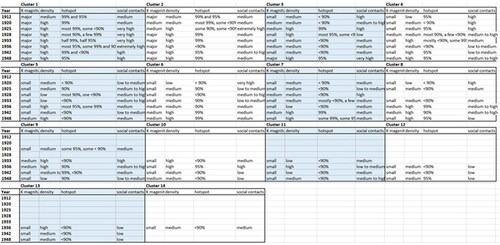
Steps 2 and 3 focus on spatial clustering. Step 4 incorporates the social network data to identify functional clusters. We scored individual clusters according to the total number of social contacts within the clusters (ranked in descendancy). In each selected year, the clusters within the top 10% (sum of social contacts) are classified as clusters of ‘high social influence’ or ‘very high influence’ or ‘extremely high influence.’ The next 30% were clusters of ‘medium influence.’ The next 35% achieved ‘low influence’ and the bottom 15 had ‘very low influence.’ We also considered high-ranking individual artists. Their presence, if any, helped to lift the cluster’s social network score into a higher rank. Table 1 explains the meaning of each category.

Table 1. Social network evaluation criteria.

Type No. Social Contacts	Social Network Node
No. of Social Contacts (ranking): Very low	Not a social network node, not a spatial cluster
No. of Social Contacts (ranking): Low	Not a social network node, not a spatial cluster
No. of Social Contacts (ranking): Medium	Medium-scale social network node, not a spatial cluster
No. of Social Contacts (ranking): High	Key social network node, not a spatial cluster

As K-function and spatial autocorrelation are time, area, and attribute specific (Baddeley, Rubak, and Turner 2015), we identified varying degrees of autocorrelation specific to years. The highest density category in 1912, for instance, may be equivalent to the lowest density category in 1936. The K function testing result classifies the K values into nine classes. Clusters of the top four classes are labeled ‘major clusters’ in our research. The ‘medium-sized cluster’ category correlates to the next two classes. The ‘small cluster’ category covers the next two classes of lower density, and the bottom class is labeled ‘tiny cluster.’ Table 2 is a matrix of social networks and spatial clustering.

Table 2. Single district-based cluster.

Spatial density No. of Social Contacts	Single District based Spatial / Lcational Cluster
	Low Density	Medium Density	High Density
No. of Social Contacts (ranking): Very low	Not a social network node, not a spatial cluster	Spatial cluster (medium density) without social network	Spatial cluster (high density) without social network
No. of Social Contacts (ranking): Low	Not a social network node, not a spatial cluster	Spatial cluster (medium density) with little social network	Spatial cluster (high density) with little social network
No. of Social Contacts (ranking): Medium	Medium-scale social network node, not a spatial cluster	Spatial cluster (medium density) with a medium degree of social networking	Spatial cluster (high density) with a medium degree of social networking
No. of Social Contacts (ranking): High	Key social network node, not a spatial cluster	Functional cluster (medium density) with vibrant social networks	High-density functional cluster with vibrant social networks

The hot spots analysis generates hot spots and cold spots. Only hot spots are discussed in this research. The result is scaled on three confidence levels, i.e., 90%, 95%, and 99% confidence levels. A combination of the afore-mentioned three dimensions leads to a cubic-shape-benchmark for cluster classification (Diagram 1).

Diagram 1. A combination of three dimensions in step 1 through step 3.

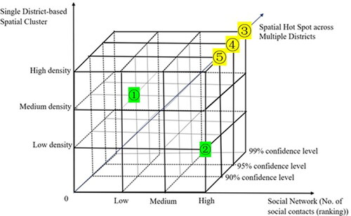
We enclose three examples for interpretation. Point 1 represents a medium-sized cluster located in a district of medium density of artists. It was a hot spot on the 90% of confidence level, which means the surrounding districts had similar density to a certain degree. The cluster, nevertheless, had a low degree of social networking. It was mostly likely a spatial cluster of junior artists or new migrants with little social impact. Point 2 exemplifies a key social network node (high-weight members) with high influence, located in a geographically peripheral area. It did not constitute a spatial cluster. That node could be one influential master who chose to reside in a marginalized locality, which hindered his followers from living closer. To identify the most influential art districts, we have focused interest in clusters that had active social networks, located in a district of high density of artists, and constituted recognizable hotspots (90% confidence level or above), as exemplified by Points 3, 4 and 5. They are defined as ‘primary functional clusters’ or ‘the most influential art districts’ in our research.

To verify our identified functional clusters, we incorporated qualitative data, e.g., biographies, archives, and other historical documents, and analyzed inter-actor interactions (e.g., types of activities and ways of communication).

Materials and methods

Our research team spent one year creating a database of Shanghai art maps. We first set up the criteria for data collection. We define ‘artist’ as practitioners of visual art, such as painters, sculptors, and calligraphers. Only artists with public profiles met our criteria for research. These artists were reported in Republican period newspapers and periodicals, documented in exhibit brochures, or recorded in art school archives⁵, and/or art organizations’ membership lists. We include all the artists that met our criteria in our database of artists’ residential addresses (created on pgadmin4). ‘Social contact’ was a person within/related to the art field that had social ties to another Shanghai artist. Evidence of interpersonal connections was uncovered through a thorough documentary search for data collection.⁶ The second database that we created stored all the pairwise inter-personal relationships of artists and their social contacts.

To find artists’ addresses and the pairwise social contacts, we collected both first-hand and secondhand historic data from 156 biographies, 22 auto-biographies, 9 types of Republican-period newspapers, 33 types of magazines, 652 academic books, 288 academic papers, 94 memories, and 57 volumes of archives housed in the Shanghai Archive House. Based on the data we collected, we came up with historical locational data for 1349 artists, and identified 1,373 pairwise social connections. To prepare spatial data, we selected two Shanghai maps, ‘Zuixin Shanghai Jieshi Tu’ (The Latest Shanghai Neighborhood Map) (1937 and 1947) on the scale of 1:20,000, from the virtual Shanghai website⁷ due to their high resolution. The datum that we used is based on the Open Street Map coordinate system. With ArcGIS 10.2, we performed heads-up digitizing and geo-registered our base maps using 50 control points each. In this process, rubber sheeting and spline transformation were used to improve the precision. Our digitalized map of 1937 comprises 1087 streets, and the 1947 map comprises 675 streets. Both are stored in the geodatabase. We also digitized four maps of varying administrative units in four years: 1908, 1926, 1928, and 1948.

We selected eight years for spatial analysis, attempting to capture historical transitions in Republican Shanghai. We start at 1912 and end at1948. 1912 is the starting year of the Republican period, and is hence selected as the starting point of our research period. Year 1920 is one year after the implementation of the national esthetic education policy. With that policy, Cai Yuanpei advocated learning art from the West, which boosted art schools and organizations in Shanghai (Zheng 2007). Year 1925 is argued to be the heyday of Western-style painting because a number of Chinese art students returned from the West (Zheng 2016). The Kuomingtang regime was established in 1928 and advocated different urban policies. We selected 1933 and 1936 (before the Sino-Japanese War) due to data availability. 1942 is a year before the Wang Jingwei administration changed the urban system and the cultural policy. It was also the year before the handover of the concessions from the imperialist power to the Chinese. 1948 was the ending year of the Republican period.

We created a point data shapefile by locating each artist on the base maps. Shanghai Commercial Guide (Hanghao Lutu Lu) published in 1937 and 1947 mapped all the residential buildings with street numbers. They provide an importance reference for our mapping of artists’ residential locations. To create pairwise social connection lines in ArcGIS, we separately compared the artists and their contacts running sql language codes in pgadmin4. The result was eight datapoint shapefiles that contain all the pairwise actors with available addresses. We then added polylines to connect the artist pairs and calculated the length of each network segment (‘calculate geometry’ function).

In the process of data analysis, we first used sql language in pgadmin4 to count the number of social contacts for each artist and ranked artists according to these numbers. Step 2 has a key parameter in kernel density estimation, the bandwidth (search radius). We first used ‘Square_Map_Units’ and then changed it into 500, 1,000, and 1,500 meters for comparison. For density and hot spot analyses, we created a map (based on the street system and administrative units), dividing the Shanghai territory into 55 sub-districts for the purpose of spatial statistics.⁸ For Objective 2, Z test and two t-tests were run using R. The codes and results are enclosed in the appendix.

Mapping the most influential art clusters in shanghai

This section reports the result of step-by-step application of the new method.

Step 1: Identifying the major functional clusters

Diagram 2 includes the top 25 artists ranked in descending order according to the number of their social contacts. We consider the top five artists as the key social network nodes in their respective years.

Diagram 2. Ranking artists per the number of their social contacts and tracing the rank changes (source: the team).

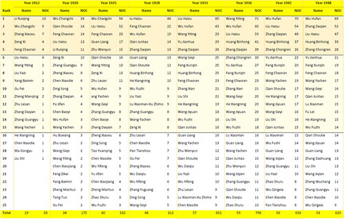
Our network type analysis shows that the top five artists on this list largely constituted the key social network nodes (with high-weight membership) except three artists (Diagram 3). Zhu Wenyun (1895-1940) was a relative and student of Wu Changshi (1844-1927) in 1928. Most of his social contacts were referred by Wu from Wu’s circle of art friends (Lu 2015; Zhu 1993). Hence, a big section of his social contacts was ‘senior art friends and teachers.’ Zhu was not an influential network node. Guan Liang (1900-1986) was a returning young artist from Japan in 1925, new to Shanghai’s cultural circle led by Mao Dun (1896-1981), Ye Shengtao (1894-1988), Zheng Zhenduo (1898-1958), and Feng Naichao (1901-1983) (Guan 1984). Most of Guan’s social networks were based on art school colleagueship (38.9%) and ties to senior non-painting cultural figures (33.3%). Hence, Guan was not an influential social network node in that year. Similarly, in 1928, 90.5% of Qian Juntao’s (1906-1998) social contacts were non-painting mentors (Qian 2007) (Table 3).⁹

Diagram 3. Percent composition of artists’ social connection types.

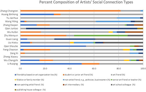
Table 3. Total number of categorized social contacts of the most popular artists.

Category of social contacts Artists	Friendship based on art organization ties	Student or junior art friend	Art friend	Relative or family member	Non-artist friend, e.g., politician, businessmen, literati	Senior art friend or mentor	Non-painting artist friend	Art intermediary	Art school colleague	Publishing house colleague	Total
Li Ruiqing	7	2	5								14
Wu Changshi		10	52	4	1	4	2	3			90
Zheng Xiaoxu	14		8								8
Zeng Xi		1	23		2		1				27
Feng Chaoran	1	8	22	2	1	1	2				37
Qian Shoutie	15		10			1		1	1		28
Liu Haisu	10	2	39	4	20	2	8	1	40		126
Guan Liang			4				6		7		18
Zhu Wenyun	1	6	1			7			2		16
Wu Hufan		15	49	3	3		6	13			89
Qian Juntao			1				19			1	21
Zhang Daqian	9	7	41			1	4	5			67
Wang Yiting	2	1	34		17		2		4		60
Yu Jianhua			33		8		1				42
Huang Binhong	15	3	37								55
Zhang Chongren		40	8		1						49

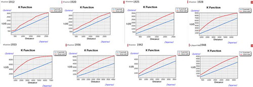
Step 2: Identifying spatial clusters using K function

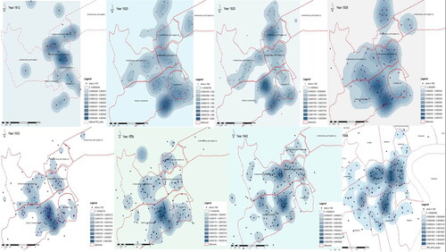
Our K function analysis reveals the artists’ densely inhabited areas, or clusters (Figure 1). The number of clusters vary from 4 (1912) to 14 (1936) across the eight years. The clusters can be classified into ‘primary cluster,’ ‘medium-sized cluster,’ ‘small cluster,’ and ‘tiny cluster’ according to our criteria addressed in ‘Objective 1, Step 4.’ Tabulation of these classifications can be found in Diagram 4.

Figure 1. K function analysis results.

Source: all maps in this project were produced by Jane Zheng with support from the team.

We also used the ‘Multi-Distance Spatial Cluster Analysis (Ripley’s K Function)’ tool to analyze the density of the clusters. The K(d) > π$d^2$ pattern applies to each of the selected years (Figure 2).

Figure 2. Ripley’s K Function statistical results.

Step 3: District-based density mapping and hot spot analysis

We located the K-function-generated spatial clusters into the system of districts that we created and calculated the density of artists in each district, as well as the hot spots (districts). The results are reported in Diagram 4.

Diagram 4. Evaluating art clusters in four dimensions, e.g., K function, single-district density, hotspot, and number of social contacts.

Step 4: Incorporating the social network dimension and mapping art clusters

In the final step, we scored each cluster on the dimension of social networks and classified the clusters according to our comprehensive evaluation.

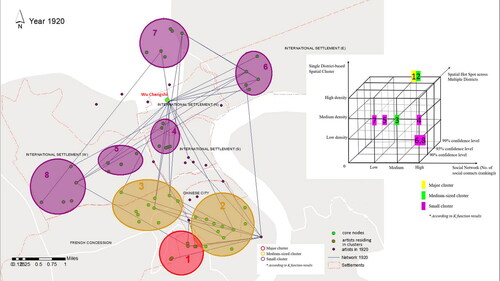
1912 and 1920 did not see the formation of clusters with vibrant social connections. Individuals with high social impacts (e.g., Wu Changshi (1844-1927)) strayed from the areas that other artists opted to live in.

One cluster that deserves attention is Cluster 3 in 1920 (located in the north-central part of the French Concession). It was an emerging functional cluster in that year, which later evolved into the biggest art cluster (1925-1948). According to our mapping, few artists lived in this area in 1912 and the cluster was not yet a hot spot by 1920, which indicates that it did border with other art clusters.

This cluster rapidly grew after Wu Hufan’s arrival in 1924. Wu, born in an imperial official’s family in Suzhou, inherited rich antique collections and moved to Shanghai. He lived next door to Feng Chaoran (1882-1954) in a lane on Gross Rue and achieved a meteoric rise in the art world (Zheng 2016). In 1925, this cluster accommodated 20 artists, including Xiong Songquan (1884-1961), Qian Shoutie (1897-1967), He Xiangning (1891-1977), Shen Maishi (1891-1986), and Teng Gu (1901-1941), in addition to Wu and Feng. Its geographic scope was roughly equivalent to Cluster 3 (1920) with a reduced spatial connection to the Chinese City.

The other major cluster is Cluster 2. Wu Changshi, the leading master, did not live in a cluster in 1920, but he attracted his followers and friends to reside in his area by 1925, leading to the formation of a medium-sized spatial cluster. Two small clusters emerged in the proximity, i.e., Cluster 6 and Cluster 8. Particularly, Cluster 8 was the area that some established artists, e.g., Huang Binhong (1865-1955), Wu Daiqiu (1879-1949), and Liang Dingming (1898-1959), resided in and all had connections with Wu Changshi. Hence, Cluster 2 emerged as a hot spot on the 90% confidence level. 19 artists lived in this cluster and most of them were within Wu Changshi’s art circle. Zhu Wenyun (1895-1939), Zhu Lesan (1902-1984), Wang Geyi (1897-1988), for instance, were relatives and art students of Wu. Mu Ruxu (1904-1996) was also Wu’s student (Zhu 2014; Liu 1986). Centering on Wu Changshi, this cluster was actually the leading social network node in 1925 despite its modest spatial occupation.

In 1928, Cluster 1 remained as the solo major functional cluster. However, Cluster 2 in 1920 (centering on Wu Changshi) disappeared as Wu passed away in 1927.

The 1930s was the golden age of art and culture in Shanghai. Multiple new clusters emerged in the foreign settlements owing to the artist population’s dramatic growth. Cluster 1 (1928) enhanced its magnetic influence and attained an even higher density in 1933. Wu Hufan and Feng Chaoran were the social network center of this cluster: the total number of their social connections account for a sizeable portion of all connections in the cluster.

The distribution pattern of 1933 reveals signs of continuity compared with 1928. Cluster 7 expanded in 1928 when new artists moved in, leading to its break into two clusters. Most artists in Cluster 7 (1928) remained in Cluster 9 in 1933, such as Zhang Hongwei (1879-1970), Zhu Qizhan (1892-1996), and Gu Fei (1907-2008). However, the geographic scope of this cluster gravitated toward Cluster 1 as some artists moved into the area between these two clusters. This caused the expansion of Cluster 9 and increased the legibility of Cluster 1 as a hot spot.

The Shanghai art world continued its booming outlook in 1936. 14 art clusters are identifiable. Cluster 1 fully established itself as the most influential art cluster, accommodating 40 artists, including Wu Hufan, the Zhang Daqian (1899-1983) brothers, Huang Binhong (1865-1955), Lu Yifei (1908-1997), Tao Lengyue (1895-1985), Wang Geyi, Feng Chaoran, Qian Shoutie, Zhang Chongren (1907-1998), Liu Haisu, Pang Xunqin (1906-1985), and the art critic, Fu Lei (1908-1966). Many of them were first-tier artists. The influence of this art center spilled over into the surrounding neighborhoods. The consequent spatial configuration is a centering position of Cluster 1 surrounded by two smaller clusters, Cluster 9 and Cluster 8¹⁰.

Cluster 10 was the other major functional cluster, located in the Chinese City and the Lao Xi Men area, the traditional yet declining base of Chinese painters. In his heyday, Wang Yiting (1867-1938) had substantial influence in this area. Artists living in these two clusters were mostly traditional-style Chinese painters and calligraphers.

In 1942, the outbreak of the Sino-Japanese War did not significantly change the pattern of artists’ spatial distribution despite the decline of the artist population size. Cluster 1 continued to be the center of Shanghai’s art world. Some artists in Cluster 9 (1936) moved closer to Cluster 1 (1936) and the two clusters approximately became one. Cluster 2 (based on Clusters 3 and 4 in 1936) rose to be the other primary art cluster in 1942.

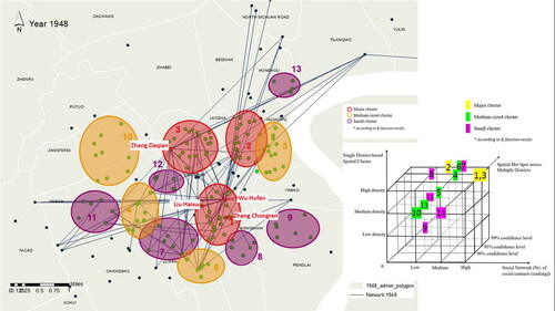
We identified 13 art clusters¹¹ in 1948. Cluster 1 maintained its leading position, surrounded by three clusters i.e., Clusters 7, 8, and 9. Yet, the density of its district went down marginally, and two other major clusters overpassed it in density. Cluster 3 evolved from Cluster 2 in 1936, centering on Li Qiujun (1899-1973) and the Li Zuhan (1891-1964) siblings’ house (No.158 Shimen Road). Zhang Daqian’s regular guest residence enhanced the social status of this locality into the range of art centers in Shanghai (Yang 2015; Li 1987). Some other established traditional-Chinese style painters, e.g., Zheng Wuchang (1894-1952), Xu Zhengbai (1877-?), Xu Bangda (1911-2012), and Yang Qingqing (1895-1957) lived in the surrounding neighborhoods.

The 11 primary art clusters that we identified are summarized in Table 4.

Table 4. A list of the 11 major art clusters.

Year	Cluster ID	Location	Number of artists
1925	1	Central-north French Concession. North: Rue Vincent Mathieu: South: Xi Men Road; West: Rue Massenet; East: Rue Lemaire; West: Marche, Rue du. It covers 22 blocks.	20
1925	2	East Zabei and north-western International Settlement: North: Xinmin Road; South: Qipu Road; East: North Sichuan Road; West: Gansu Road. It covers 16 blocks.	19
1928	1	Central-north French Concession: North: Rue Du Consulat, South: Ximen Road; West: Rue Massenet; East: Rue Lemaire; West: Marche Rue du. It covers 22 blocks.	13
1933	1	Same as Cluster 1 in 1928	27
1933	9	South and north sides across the International and French Concession border: North: Weihaiwei Road; South: Valon Route; West: Moulmein Road; East: North Chengtu Road. It covers 8 blocks.	16
1936	1	Same as Cluster 1 in 1928	40
1936	10	Eastern part of the walled city	9
1942	1	Central-north French Concession: North: East Chungcheng Road; South: Rue de la Observatoire; West: Northern Chungcheng Road (II); East: Rue Lemaire; West: Marche Rue du. It covers 26 blocks.	41
1942	2	East-North International Settlement: South: Bubbling Well Road; North: Avenue Road; East: Changsha Road; West: Tatung Road. It covers 8 blocks.	27
1948	1	Same as Cluster 1 in 1928	27
1948	3	Central-North International Settlement: North: Xinzha; South: West Nanjing Road; East: Changjiang Road; West: Zhongzheng Road (II). It centers on Shimen Road (II).	27

Discussions

We discuss the characteristics of the major art clusters that we identified by incorporating qualitative data into our findings.

First, there were partial correlations between the dynamics of the social networks of the artists and the transformation of art clusters. The structure of artists’ social networks changed during the course of the historical period; some artists rapidly achieved popularity and moved up the ranks, while others slowly accumulated networks and moved down the ranks (Diagram 2). Similarly, the spatial distribution pattern of artists underwent transformations; some clusters grew while other declined (Figures 3–9). The changes in the two distinctive dimensions partially matched each other. Some artists with substantial social networks chose to live in sequestered places and were not helpful to grow clusters. The death of a leading artist of a cluster usually led to the demise of the cluster, but in some exceptional cases, the master’s followers restored the cluster (e.g., Wu Changshi). When artists with social influence resided in areas under suitable social and geographic conditions, they could contribute to the formation of clusters (e.g., Wu Hufan). In such cases, the locality also benefited the social networks of the artists. Hence, the network-cluster correlation was a dialectic relationship.

Figures 3. Art cluster mapping, 1920.

Figures 4. Art cluster mapping, 1925.

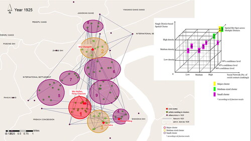
Figure 5. Art cluster mapping, 1928.

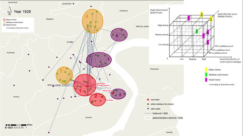
Figure 6. Art cluster mapping, 1933.

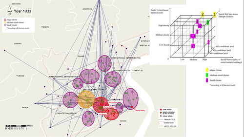
Figure 7a. Art cluster mapping, 1936.

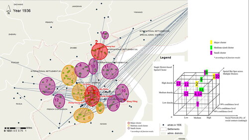
Figure 7b. Individual artists residing in the primary art cluster, 1936.

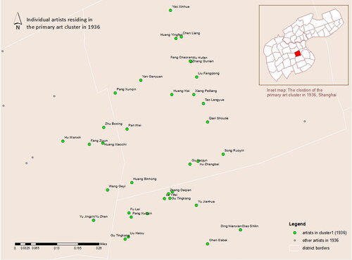
Figure 8. Art cluster mapping, 1942.

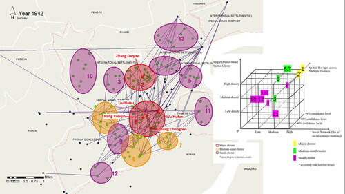
Figure 9. Art cluster mapping, 1948.

Moreover, primary clusters may comprise multiple nodes based in neighborhoods. Cluster 1, for instance, is found to be composed of a number of inter-related art neighborhoods. In addition to Wu Hufan and Feng Chaoran’s residential quarter, Liu Haisu’s residence was another center connecting artists in his circle.¹² Li Yishi (1886-1942), who moved to Shanghai at Liu’s invitation, was appointed as the head of teaching affairs at the Shanghai Art College in 1924. Li’s family lived in a nearby neighborhood and often visited Liu (Li 2010). Zhang Chongren (1907-1998) was a European academy-trained returning sculptor. He set up his studio at No. 608 Pé190Froc Rue Du in 1936; it was the first sculpture studio of this type in Shanghai. He successfully attracted and groomed the first generation of sculpture students (Chen 2003). The geographic concentration of such sub-communities enabled this major cluster to become the most influential art district of the city.

Conclusion

Our identification of the major art clusters is partially echoed by previous qualitative research, which recorded Republican period Shanghai artists’ residential and socializing activities. Nonetheless, as the first research that adopts computer-facilitated quantitative research methods (e.g., historic GIS and R for spatial statistical analysis) for the field of Twentieth-century Chinese art history, we have provided scientific proofs for the clusters that we identified. Also, most historical research is biased toward artists with recognizable achievements in the contemporary vision; less famous artists are often neglected. Our research maps the spatial clustering of the less famous artist group based on their addresses. Further, our findings have corrected some misunderstandings in modern Shanghai art history. Most scholars who wrote about the Shanghai artists’ spatial distribution pattern assumed that the surrounding neighborhoods of the Shanghai Art College, i.e., Lao Xi Men area, were the primary cluster. Our research, however, shows Lao Xi Men was the medium-sized cluster and it declined in the 1930s. Instead, the North-central French Concession stood as the biggest art cluster from 1925 to 1948.

The method for cluster mapping proposed in this paper comprehensively evaluates art clusters in four dimensions, blending spatial density and social network analyses. Thus, it develops sophisticated classification of art clusters by differentiating their performances on the spatial dimension versus social networking. This model is tailored to historical art or cultural clusters better than any of the previous mapping methods.

The mapping results described in this paper sets in train a research agenda about possible social historical conditions that led to the particular spatial distribution patterns of artists in Republican Shanghai. We speculate about the favorable environmental attributes to artists, including economic growth, a prosperous outlook of the financial and real estate sectors. Artists flocked into the concessions for employment, art consumption and decent housing. The extraterritorial rights of the concessions ensured a low intervention level of the authorities and high latitude of expression and artistic pursuits. The concessions were also the refuge for artists during the warfare. Urban transport and amenities enhanced the convenience of commuting and added modern city charms. We call for further research to test these hypothesized contributing environmental attributes for an improved understanding about a conducive environment for art production.¹³

Acknowledgement

The authors are grateful to the two anonymous reviewers and the handling journal editor. Seven graduate students from the School of Architecture at Tianjin University participated in the GIS mapping for this project. Ms. Guo Xiaomin was the leading contributor and coordinator in the student group. Ms. Wang Chaoqun and Mr. Xiao Tianyi contributed to visualizing the spatial data while the rest four students did data processing. We also thank Dr. Rashmila Maiti for the final check.

Disclosure statement

No potential conflict of interest was reported by the authors.

Additional information

Funding

This research was funded by the Hong Kong Research Council GRF research grant (CUHK14621516). UW–Madison provided additional funding for open access.

Notes

1 The Shanghai Art College (1913-1952) was the most influential private art school in Republican Shanghai. For the history of the College, see Zheng (2016).

2 The principle that art venues avail social networking applies to Republican Shanghai, a city that embraced abundant modern art facilities (Hay 2001).

3 For our criteria, see the ‘materials and methods’ section.

4 As the first research of mapping art clusters in Republican Shanghai, we are most concerned with the artists with substantial social contacts. Hence, we have simplified the centrality analysis in network analysis.

5 Art school yearbooks, graduation books, and pay rolls contain substantial address information.

6 See the next paragraph.

7 https://www.virtualshanghai.net/

8 Police districts or school districts data are not available.

9 Within the ten categories of artists’ social contacts, ‘friendship based on art organization ties’ refers to the friendship that evolved based on artists’ association with some common art organizations. ‘Student or junior art friend’ indicates that the social contact was the artist’s student or follower. It was a master-student relationship. ‘Art friend’ refers to a bond with mutual affection; the social relationship was based on shared interests in art on equal foot stands. ‘Relative or family member’ is a type of direct social relationship, referring to family members devoted to art. ‘Non-painting artist friend’ is one type of friendship between artists; the contact, however, was not a painter, but other art sectors. ‘Non-artist friend’ was not an artist, but a person active in other circles, such as politics and businesses, with interest caring about art-related affairs. ‘Art intermediary’ was engaged in art businesses, such as mounting shops, fan shops, and was associated with the artist due to art business interests. ‘Art school colleague’ and ‘publishing house colleague’ were two types of social relationships based in institutions.

10 Artist faculties of the Shanghai Art College concentrated in this area.

11 The K function analysis reveals three additional small clusters, each including two or three artists. Being low in significance, they are not represented on our map.

12 Liu acted as the principal of the Shanghai Art College for nearly forty years.

13 Our recent effort to explore the cause and effect of the Republican Shanghai art scene is reflected in an upcoming paper, see Zheng et al. (2022).

References

- Abfalter, Dagmar, and Martin Piber. 2016. “Strategizing Cultural Clusters: Long-Range Socio-Political Plans or Emergent Strategy Development?” The Journal of Arts Management, Law, and Society 46 (4):177–86. doi: 10.1080/10632921.2016.1211051.
- Aguilar, Glenn D., and Mark J. Farnworth. 2012. “Stray Cats in Auckland, New Zealand: Discovering Geographic Information for Exploratory Spatial Analysis.” Applied Geography 34:230–8. doi: 10.1016/j.apgeog.2011.11.011.
- Baddeley, Adrian, Ege Rubak, and Rolf Turner. 2015. Spatial Point Patterns: Methodology and Applications with R. Boca Raton, FL: CRC press.
- Bol, Peter K., and Jianxiong Ge. 2005. “China Historical GIS.” Historical Geography 33:150–2.
- Castells, Manuel. 2004. “Informationalism, Networks, and the Network Society: A Theoretical Blueprint.” In The Network Society: A Cross-Cultural Perspective, edited by Manuel Castells, 3–45. Northampton, MA: Edward Elgar.
- Chen, Yaowang. 2003. Nisu Zhi Shengshou ye: Zhang Chongren de Yishu Rensheng [Highly Skilled Practitioner of Sculpturing: The Art Life of Zhang Chongren]. Shanghai: Shanghai wenyi chubanshe.
- Christopherson, Susan. 2002. “Project Work in Context: Regulatory Change and the New Geography of Media.” Environment and Planning A: Economy and Space 34 (11):2003–15. doi: 10.1068/a34182.
- Ettlinger, Nancy. 2003. “Cultural Economic Geography and a Relational and Microspace Approach to Trusts, Rationalities, Networks, and Change in Collaborative Workplaces.” Journal of Economic Geography 3 (2):145–71. doi: 10.1093/jeg/3.2.145.
- Evans, Graeme. 2004. “Cultural Industry Quarters: From Pre-Industrial to Post-Industrial Production.” In City of Quarters, edited by Mark Jayne and David Bell. London: Routledge.
- Fischer, Manfred M., and Arthur Getis. 2010. Handbook of Applied Spatial Analysis: Software Tools, Methods and Applications. Berlin, Heidelberg: Springer-Verlag Berlin Heidelberg.
- Fleming, Tom. 2004. “Supporting the Cultural Quarter? The Role of the Creative Intermediary.” In City of Quarters: Urban Villages in the Contemporary City, edited by Mark Jayne and David Bell, 93–108. London: Routledge.
- Fotheringham, A. Stewart, Chris Brunsdon, and Martin Charlton. 2000. Quantitative Geography: Perspectives on Spatial Data Analysis. London: Sage.
- Gao, Song, Krzysztof Janowicz, and Helen Couclelis. 2017. “Extracting Urban Functional Regions from Points of Interest and Human Activities on Location-Based Social Networks.” Transactions in GIS 21 (3):446–67. doi: 10.1111/tgis.12289.
- Gardner, Howard E. 1993. Creating Minds: An Anatomy of Creativity Seen through the Lives of Freud, Einstein, Picasso, Stravinsky, Eliot, Graham, and Ghandi. New York: Basic Books.
- Girvan, Michelle, and Mark E. J. Newman. 2002. “Community Structure in Social and Biological Networks.” Proceedings of the National Academy of Sciences of the United States of America 99 (12):7821–6. doi: 10.1073/pnas.122653799.
- Gordon, Ian R., and Philip McCann. 2000. “Industrial Clusters: Complexes, Agglomeration and/or Social Networks?” Urban Studies 37 (3):513–32. doi: 10.1080/0042098002096.
- Granovetter, Mark S. 1973. “The Strength of Weak Ties.” American Journal of Sociology 78 (6):1360–80. doi: 10.1086/225469.
- Griffith, Daniel. 1987. Spatial Autocorrelation. A Primer. Washington, DC: Association of American Geographers.
- Guan, Liang. 1984. Guan Liang Huiyi Lu” [Memories of Guan Liang], edited by Guanfa Lu, vol. 9, 29–44. Shanghai: Shanghai Shuhua Chubanshe. (in Chinese).
- Hall, Peter. 2000. “Creative Cities and Economic Development.” Urban Studies 37 (4):639–49. doi: 10.1080/00420980050003946.
- Kumar, Ravi, Prabhakar Raghavan, Sridhar Rajagopalan, Dandapani Sivakumar, Andrew Tompkins, and Eli Upfal. 2000. “The Web as a Graph.” In Proceedings of the Nineteenth ACM SIGMOD-SIGACT-SIGART Symposium on Principles of Database Systems, 1–10.
- Langlois, Richard N., and Paul L. Robertson. 1995. Firms, Markets and Economic Change: A Dynamic Theory of Business Institutions. London; New York: Routledge.
- Lazzeretti, Luciana, Rafael Boix, and Francesco Capone. 2008. “Do Creative Industries Cluster? Mapping Creative Local Production Systems in Italy and Spain.” Industry & Innovation 15 (5):549–67. doi: 10.1080/13662710802374161.
- Lee, Leo Ou-fan, and Oufan Li. 1999. Shanghai Modern: The Flowering of a New Urban Culture in China, 1930–1945. Cambridge, MA: Harvard University Press.
- Liu, Haisu, ed. 1986. Huiyi Wu Changshi [Commemorating Wu Changshui]. Shanghai: Shanghai renmin meishu chubanshe. (in Chinese).
- Li, Yongqiao. 1987. Zhang Daqian Nianpu [the Chronology of Zhang Daqian]. Chengdu: Sichuan Science Academy Press.
- Li, Zongshan, and Yunfang Fang. 2010. “Huiyi wo de fuqin Li Yishi" [Commemorating My Father Li Yishi]. Shilin A1:62–7. (in Chinese).
- Lin, Zhuo. 2018. “Ershi Shiji Qianqi Shanghai Lao Xi Men Diqu Xiyang Huodong Yanjiu” [Study on Early 20th Century Western Style Painting Activities at Shanghai Laoximen].” PhD diss., Shanghai: Shanghai University. (in Chinese).
- Love, James H., and Stephen Roper. 2001. “Location and Network Effects on Innovation Success: Evidence for UK, German and Irish Manufacturing Plants.” Research Policy 30 (4):643–6. doi: 10.1016/S0048-7333(00)00098-6.
- Lu, Xin. 2015. “Xiaosa Qingyi, Shebi Chengqu: Zhu Wenyun Xiansheng Jishi” [Fresh and Elegant Brushwork: Stories of Mr.Zhu Wenyun].” Shuhua Yishu 3:57–67. (in Chinese).
- Markusen, Ann. 2006. “Urban Development and the Politics of a Creative Class: Evidence from a Study of Artists.” Environment and Planning A: Economy and Space 38 (10):1921–40. doi: 10.1068/a38179.
- Marsden, Peter V. and Karen E. Cambell. 1984. “Measuring Tie Strength.” Social Forces 63 (2):482–501.
- Martí-Costa, Marc, and Marc Pradel I. Miquel. 2012. “The Knowledge City against Urban Creativity? Artists’ Workshops and Urban Regeneration in Barcelona.” European Urban and Regional Studies 19 (1):92–108. doi: 10.1177/0969776411422481.
- Mommaas, Hans. 2004. “Cultural Clusters and the Post-Industrial City: Towards the Remapping of Urban Cultural Policy.” Urban Studies 41 (3):507–32. doi: 10.1080/0042098042000178663.
- Montgomery, S. Sarah and Michael D. Robinson. 1993. “Visual Artists in New York: What’s Special about Person and Place?” Journal of Cultural Economics 17 (2):17–39.
- Ng, Michael, T. Edwin Chow, and David W. S. Wong. 2016. “Geographical Dimension of Colonial Justice: Using GIS in Research on Law and History.” Law and History Review 34 (4):1027–45. doi: 10.1017/S073824801600033X.
- Ord, J. Keith, and Arthur Getis. 2010. “Local Spatial Autocorrelation Statistics: Distributional Issues and an Application.” Geographical Analysis 27 (4):286–306. doi: 10.1111/j.1538-4632.1995.tb00912.x.
- Papadopoulos, Symeon, Yiannis Kompatsiaris, Athena Vakali, and Ploutarchos Spyridonos. 2012. “Community Detection in Social Media.” Data Mining and Knowledge Discovery 24 (3):515–54. doi: 10.1007/s10618-011-0224-z.
- Perry, Martin. 2005. Business Clusters: An International Perspective. New York: Routledge.
- Porter, Michael E. 2000. “Location, Competition, and Economic Development: Local Clusters in a Global Economy.” Economic Development Quarterly 14 (1):15–34. doi: 10.1177/089124240001400105.
- Preissl, Brigitte, and Laura Solimene. 2003. Dynamics of Clusters and Innovation. Heidelberg, Germany: Physica-Verlag.
- Qian, Juntao. 2007. “Qian Juntao Nianbiao” [Chronology of Qian Juntao].” In Qian Juntao Jinian Ji [Collection of Memorial Articles on Qian Juntao], edited by Shanghai lu xu memorial house. Shanghai: Zhongguo fuli hui chubanshe. (in Chinese).
- Roodhouse, Simon. 2006. Cultural Quarters: Principles and Practice. Bristol, UK; Portland, OR: Intellect Books.
- Roodhouse, Simon. 2010. Cultural Quarters: Principles and Practice. Bristol: Intellect Books.
- Saleh, Imane Ali., and Perumal Balakrishnan. 2019. “GIS Based Hotspot and Cold-Spot Analysis for Primary Education in India.” Indian Journal of Science and Technology 12 (45):1–33. doi: 10.17485/ijst/2019/v12i45/148448.
- Scott, Allen J. 2004. “Cultural-Products Industries and Urban Economic Development: Prospects for Growth and Market Contestation in Global Context.” Urban Affairs Review 39 (4):461–90. doi: 10.1177/1078087403261256.
- Scott, AllenJ. 2000. The Culture Economy of Cities: Essays on the Geography of Image Producing Industries. London: Saga.
- Taylor, Nora A. 2016. “Have Performance, Will Travel: Contemporary Artistic Networks in Southeast Asia.” Asian Journal of Social Science 44 (6):725–39. doi: 10.1163/15685314-04406006.
- Tremblay, Diane-Gabrielle, and Elisa Cecilli. 2009. “The Film and Audiovisual Production in Montreal: Challenges of Relational Proximity for the Development of a Creative Cluster.” The Journal of Arts Management, Law, and Society 39 (3):156–86. doi: 10.1080/10632920903218539.
- Ulldemolins, Joaquim Rius. 2012. “Gallery Districts of Barcelona: The Strategic Play of Art Dealers.” The Journal of Arts Management, Law, and Society 42 (2):48–62. doi: 10.1080/10632921.2012.678929.
- Wasserman, Stanley, and Katherine Faust. 1994. Social Network Analysis: Methods and Applications. 1st ed. Cambridge; New York: Cambridge University Press.
- Xu, Hongxin. 2015. “Shanghai Meizhuan Zhoubian Chengqu Yanjiu” [a Study of the Surrounding Neighborhood of the Shanghai Art College].” In Buxi de Biandong: Shanghai Meizhuan Jianxiao 100 Zhounian Guoji Yantao Hui [Restless Transitions: 100 Anniversary of the Shanghai Art College International Conference], edited by Liu Haisu Art Museum, 84–108. Hangzhou: Xilin yinshe chubanshe. (in Chinese).
- Xu, Xiaowei, Nurcan Yuruk, Zhidan Feng, and ThomasAJ. Schweiger. 2007. “Scan: A Structural Clustering Algorithm for Networks.” In Proceedings of the 13th ACM SIGKDD International Conference on Knowledge Discovery and Data Mining, 824–33. doi: 10.1145/1281192.1281280.
- Yang, Xiaoyun. 2015. “Zhang Daqian Nüxing Jiaoyou yu Yishu Chuangzuo” [Zhang Daqian’ Art and His Social Interactions with Women].” Master diss., Nanjing: Nanjing University of the Arts. (in Chinese).
- Zhang, Peiyao, David W. Wong, Billy K. L. So, and Hui Lin. 2012. “An Exploratory Spatial Analysis of Western Medical Services in Republican Beijing.” Applied Geography 32 (2):556–65. doi: 10.1016/j.apgeog.2011.07.003.
- Zheng, Jane, Zhang, Sabrina P.Y., Fan, Zhen, Lin, Hui, and Leung, Yuen Sang. 2022 (forthcoming). “Rediscovering Shanghai Modern: Chinese Cosmopolitanism and The Urban Art Scene, 1912–1948.” Urban History. doi: 10.1017/S096392682200027X
- Zheng, Jane. 2007. “A Local Response to the National Ideal: Aesthetic Education in the Shanghai Art School (1913-1937).” Art Criticism 22 (1):29–57.
- Zheng, Jane. 2016. The Modernization of Chinese Art: The Shanghai Art College, 1913-1937. Leuven, Belgium: Leuven University Press.
- Zheng, Jane. 2018. “Normative Approaches in Making Cultural Quarters and Assessment of Creative Industry Parks in Shanghai.” Journal of Architecture and Urbanism 42 (2):134–48. doi: 10.3846/jau.2018.6212.
- Zheng, Jane, and Roger Chan. 2013. “A Property-Led Approach to Cluster Development:’creative Industry Clusters’ and Creative Industry Networks in Shanghai.” Town Planning Review 84 (5):605–32. doi: 10.3828/tpr.2013.32.
- Zhu, Guantian, ed. 2014. Wu Changshi Nianpu Changbian [a Drafted Chronology of Wu Changshi]. Hangzhou: Zhejiang guji chubanshe. (in Chinese).
- Zhu, Han. 1993. “Mianhuai Zhongbo Zhu Wenyun” [Commemorating My Second Uncle Zhu Wenyun].” Yiyuan 1:14–5. (in Chinese).