Multidimensional inverse heat conduction problems solution via lagrange theory and model size reduction techniques

Abstract

This article is concerned with inverse heat conduction problems (IHCP) involving large-scale linear systems (i.e. multidimensional systems) with unknown sources or boundary conditions. The inverse problem is stated as an optimisation problem with a regularised quadratic objective functional, and it is solved using Lagrange theory. We demonstrate that the IHCP solution is obtained by simple time integration of a state-variable model: the inverse model, which is analytically derived from the so called direct and adjoint problems. In addition, we show that the number of differential equations in the inverse model can be strongly reduced without a significant loss of precision. The inversion is then carried out in three main steps: calculation of the full-order inverse model, size reduction, and time integration of the resulting reduced-order inverse model. A numerical example of heat sources identification in a 2D diffusion problem shows the performances and the accuracy of the proposed approach.

Keywords:

• Multidimensional IHCP
• Lagrange theory
• Reduction techniques

Introduction

The direct heat conduction problems are concerned with the determination of temperature at the interior points of a region when the initial and boundary conditions, thermophysical properties and heat generation are specified. In contrast, the inverse heat conduction problem (IHCP) involves the determination of the surface conditions (temperature or heat flux), energy generation or thermophysical properties from the temperature measurements taken at a finite number of points within the body.

Although the formulation and the first attempt to solve the IHCP were presented over a century ago, it has grown rapidly as a research subject only during the last two decades or so. An excellent review and comprehensive bibliography on the topic may be found in the books of Beck et al. [1], Alifanov [2] and Dinh [3]. The main difficulty with inverse problems is due to their ill-posed character, in the sense of Hadamard [4]. That is, they may have no solution, or if a solution exists, it may be not unique or not continuous with respect to the given data (the solution is very sensitive to the measurements noise and to the modelling errors). To overcome such a difficulty a large variety of techniques have been proposed to regularise these problems. For example, Beck [5] introduced the “function specification method” for IHCP, while Murio [6] developed the “mollification technique” to obtain smooth solutions of various inverse problems. Both approaches are simple in concept and have sequential aspects. Tikhonov, Alifanov, and other from the Russian school proposed to cast the ill-posed inverse problem into an optimisation problem with a regularised objective functional, and/or a self-regularising algorithm of solution [8–22], including IHCP, as well as problems of parameters determination and shape identification. However, the generality comes at the expense of greater computational and programming burdens. It must be noticed that such methods involve the numerical integration of three sets of partial differential equations: the so called direct, adjoint and sensitivity problems. Moreover, iterative search algorithms as the conjugate gradient method are required.

The aim of this article is to improve the computational efficiency of the Tikhonov regularisation method for IHCP concerning large-scale linear systems (i.e. multidimensional) with unknown sources or boundary conditions. This objective is reached via both the Lagrange theory for dynamic optimisation with constraints and the so called model reduction techniques.

The Lagrange theory is used to provide an analytical solution of the IHCP for linear systems with a quadratic objective functional. We demonstrate that there is a linear state-variable model (the inverse model in the following) so that the solution of the IHCP is obtained by simple time integration of it. The inverse model is analytically derived from the so called direct and adjoint problems. Neither iterative algorithms such as the conjugate gradient method nor sensitivity problem solving are required.

For large-scale systems (i.e. multidimensional problems), additional numerical difficulties may be encountered due to the dimension of the matrices to be manipulated. To overcome such difficulties, the use of reduction techniques has been recently proposed in [23–26]: first, the size of the direct model is reduced; then, the inverse problem is solved using the reduced-order direct model instead of the full-order one. We show that better results can be however achieved when reducing the inverse model directly. The inversion is then carried out in three main steps: calculation of the full-order inverse model, size reduction, and time integration of the resulting reduced-order inverse model. Due to the characteristics of the inverse model (two-point boundary-value problem), a special method for its size reduction is also proposed.

A numerical example of heat sources identification in a 2D diffusion problem is finally used to show the performance and the accuracy of the approach we are proposing for large-scale IHCP solving.

Linear Systems and Inverse Problem Statement

Let Ω be a geometrically bounded thermal system in ℜ³. We denote by Ω_o the points within the system and ∂Ω those located at its boundary surface (). It is assumed that the system domain Ω can be split-up in a finite number of solid sub-domains with invariant geometry. Each one of the sub-domains is formed by a continuous and mono-phase medium whose thermophysical properties (thermal conductivity, density and specific heat) are space continuous functions. Furthermore, such properties are assumed to be time invariant and independent of the temperature.

Direct Model

In the framework of the previous hypothesis, the thermal state T(M, t) of the system at any time t and any point , is completely determined by:

where and are respectively the spatial heat operator and the boundary conditions operator, ψ(M, t) represents the forcing functions field (solicitations) and c(M) is the heat capacity at point M.

The spatial heat operator is given by:

where k(M) represents the thermal conductivity at point M. The boundary conditions operator can be generally written as:

Dirichlet conditions are obtained for , while Neumman conditions come from . As the type of boundary conditions does not modify neither the IHCP formulation nor the IHCP solving procedure, no distinction is made in the following among prescribed heat flux, prescribed temperature or convective boundary conditions.

The solicitations field ψ(M, t) is given by:

where σ(M, t) represents the heat sources or sinks intensity within the body, ϕ(M, t) is the prescribed heat flux at the boundary, and T_∞ (M, t) is the environment temperature (or the prescribed temperature when ).

Inverse Problem Statement

We denote by Z(M, t) the problem unknowns to be determined by the inverse analysis. They can be any of the following quantities:

	the heat sources intensity within the system, σ(M, t) (the sources location is assumed to be known);
	the prescribed temperatures at the boundary surface, T∞ (M, t);
	the prescribed heat flux on the boundary surface, ϕ(M, t); or
	the convective term .

We assume that there are q temperature sensors located at the positions for which temperature observations are available at times . We denote by the temperature field verifying Eq. (1) for given values of the problem unknowns Z(M, t).

The aim of the inverse analysis is to find Z(M, t) so that the criterion:

is minimised. α(M) and β(M) are continuous functions for weighting, respectively, the residuals (differences between simulations and temperature measurements) and the unknowns. is the Dirac distribution and is a Tikhonov regularisation parameter. It allows to reduce the effect of measurements noise on the Z(M, t) estimations. Although zero-, first- and second-order Tikhonov regularisations exist, this article focuses on the zero-order.

We notice that the solicitations field can be split-up into a known term and a unknown one: . So, the temperature field can be written as (superposition principle – for linear systems only): . The first term represents the system response to , and the second one is the system response to . Hence, the objective of the inverse analysis can be defined as a function of by replacing by and by in Eq. (5). To avoid a cumbersome notation, and is assumed in the following.

The Inverse Problem Solution

To solve the continuous minimisation problem (5), Lagrange multipliers are usually used to adjoint the constraints (1) to the performance index (5). This leads to the extended criterion:

where is the Hamiltonian of the problem:

The Lagrange theory shows that the constrained minimum of is attained at the unconstrained minimum (cf. [27]). The necessary conditions for a minimum can then be easily derived.

The Necessary Conditions for a Minimum

The minimum of the function is achieved when the increments are zero for all independent increments in its arguments (T, λ, Z and t). Applying calculus of variation rules on Eq. (6), it can be demonstrated that the necessary conditions for a minimum are (see Annex, Proof 1):

So, the unknowns Z(M, t) we are looking for come from the three following problems:

1. The direct problem (from Eqs. (7) and (8a)). It is defined by

    with . When the problem unknowns are the heat sources in Ω, then ; otherwise, .

2. The adjoint problem (from Eqs. (7), (8b) and (8c)). It is defined by

   with . and are, respectively, the adjoint operators of and . The residuals act as source terms in Eq. (10); clearly, with no residuals, the adjoint problem has zero solution. We note that in the adjoint problem, the time is measured backwards from the final time t_f to the initial time .

3. The stationarity condition (from Eqs. (7) and (8d))

   This equation shows that the unknowns we are looking for are linear functions of the adjoint field.

The ICHP Solution

Since no general theory is currently available for the analytic solution of partial differential equations, approximate methods and numerical solutions are the only practical alternative to which scientist and engineers usually resort in order to solve this type of equations. The spatial discretisation of Eqs. (9)–(11) leads to a finite dimensional formulation of the general form:

with and . T(t) [] and [] are respectively the thermal state vector and the so called co-state vector (n is the number of nodes in the discretisation mesh). Their time derivatives are represented by and . Z(t) [ ] is the discrete version of the unknown field Z(M, t). Q [] and R [ ] are positive definite matrices (q is the number of sensors), they come from the discretisation of the weighting functions α(M) and respectively. Matrices A [] and E [] result from the discretisation of the spatial operators and , and and are their corresponding adjoints (transposed matrices). The matrix J [] is formed by zeros and ones; as the Dirac distribution in Eq. (10), it serves to select the points within the system where the temperature is measured.

Introducing the stationarity condition (14) in the direct problem (12) yields to the following two-point boundary-value problem:

This problem can be easily solved using the “sweep method” [28], which assumes that and satisfy an affine relation like for some as yet unknown matrix function S(t) and vector function v(t). The solution of the inverse problem is then given by (see Annex, Proof 2):

with

and and . The time-varying matrix K(t) is called Kalman gain. It is given by:

where S(t) is the unique solution of the Ricatti equation:

For a long enough time interval (infinite horizon problem), the solution of the Ricatti equation above converges to a limiting solution S_∞ :

and the Eqs. (16) and (17) become:

with .

The solution of the IHCP is hence obtained by time integration of the inverse model defined by Eq. (21). Step-by-step, IHCP solving involves:

1. Calculation of the time-invariant matrices S_∞ and K_∞ . We note that they are independent on the system state trajectory, so they can be calculated off-line.

2. Calculation of v(t) by time-integration of the equation , with . We note that the time is measured backwards from the final time t_f to the initial time . However, by defining a new time variable , the corresponding domain becomes from to t_f .

3. Calculation of T(t) by time-integration of the equation , with .

4. Calculation of

Using Reduction Techniques in the IHCP Solving

The resolution of the IHCP involves the time integration of two coupled state-variable models (see Eq. (21)), which includes as many ordinary differential equations than there are capacitive nodes in the discretisation mesh. Consequently, their size increases with the complexity and the dimension of the system geometry, as well as with the accuracy we are looking for. Inverse analysis could then be computationally intensive and limited by computer performance. In order to handle such kind of problems, an approximation based on model size reduction techniques is here proposed.

The objective of model size reduction techniques is to replace a state-variable model of high dimension by a low-dimension one without a significant loss of precision. A satisfactory representation of the full-dimension model behaviour is then achieved with a limited number of calculations. In this section, we first introduce the principles of model reduction techniques; then, two different ways of using them in the framework of the IHCP are presented and discussed.

Principles of Model Reduction Techniques

Model reduction has been the subject of many investigations and a great number of reduction techniques have been proposed in the past. A rather complete state of the art of model reduction in thermal analysis is brought in [29]. The most efficient reduction techniques are the so-called spectral methods. They consist in representing the state variables of the problem as a linear combination of the eigen-functions of a particular basis. If the projection basis allows us to highlight a small number of significant directions, the solution can then be approached using a reduced number of eigen-elements. Let

be a state-variable model of dimension n. X(t) is the state-variables vector [], U(t) is the inputs vector [ ] and Y(t) is the output vector []. F [], B [] and O [] are, respectively, the state matrix, the command matrix and the output matrix. A reduced r-order model is obtained by the following procedure:

1. Separation of the pseudo-steady and dynamic terms of the state variables: . The pseudo-steady term represents the state variables behaviour when the thermal capacity of the system is assumed to be zero. It follows that: . So, the dynamic term and the outputs verify:

   Using the formulation (23) instead of Eqs. (22) presents some clear advantages for model reduction purposes. Practice indicates that to yield accurate results for small values of r it is often necessary starting reduction from Eq. (23). Otherwise, the convergence rate with r will be much lower (cf. [29]).

2. Calculation of a pertinent equivalent full-order model. Let P be a non-singular matrix of dimension [] containing, column wise placed, the vectors of a given basis. Let us consider the similar transformation , where is the vector [] of the decomposition coefficients of on the chosen basis. From Eq. (23), it follows the equivalent model:

   with (state matrix), (command matrix), (output matrix), and (static gains matrix).  From a numerical point of view, the simplest similar transformation is the modal basis. It is defined by the following eigenvalues problem:
   is a diagonal matrix formed by the eigenvalues of F which are closely related to the time constants of the system, . Modal basis has been widely used in the past for studying a vast class of diffusion problems by analytical approaches (cf. [30]) as well as for model reduction purposes (cf. [29]). However, practice indicated that the selection of the transformation matrix P has a significant influence on the quality of the resulting low-dimension model. In this sense, the transformation leading to the so called balanced realisation of (23) is one of the best choices (see Annex for formal definition and calculation matters). The theory of balanced realisations was introduced by Moore [31] in 1981, and is based on the central notions of observability and controllability. P is chosen so that the controllability gramian and the observability gramian of the state variable model (24):
   verify:
   where are the Hankel singular values of the system, which are fundamental invariant parameters of it. The controllability gramian measures the sensitivity of the state-variable to the forcing functions while the observability gramian brings a way for measuring the sensitivity of the model outputs to the state variables. The balanced realisation of Eq. (23) is a state-variable model where state variables show equal degree of controllability and observability.

3. Full-order model truncation. Assuming vectors have been ordered in a convenient way, a reduced-order model of dimension r is then obtained as

   where the state matrix [] is formed by the r first columns and rows of , the command matrix [] includes the first r rows of , and the output matrix [] is formed by the first r columns of .  Model (27) can be rewritten as:
   with . The equivalence between models (27) and (28) may be easily verified splitting-up the state-variable vector in Eq. (27) into a pseudo-steady and dynamic terms.

In the framework of modal analysis, different criteria for eigenfunctions ordering have been proposed in the past (cf. [29]). The simplest one leads to keep the state variables in model (24) that are associated to the greatest time constant of the system [32]. Obviously, the reduced model calculated in this way will work better at low frequencies than at high frequencies for slow state variables are privileged. One of the major advantages of this technique is however its simplicity.

In the framework of balanced realisation, truncation is performed by keeping the more controllable and observable state variables in Eq. (24), those associated to the greatest r Hankel singular values (Moore’s method, [31]). It has been proved in [33] that the L_∞ -norm of the error introduced by truncation of the balanced realisation can be bounded by “twice the sum of the tail” of the Hankel singular values spectrum:

where and are, respectively, the transfer functions matrix of the full-order and the r-order models. This error bound gives strong theoretical support to the observation that truncated balanced realisations so as give very good results in practice.

Application to the IHCP – I: Direct Model Reduction

Until now, reduction techniques have been used in a very conventional way for inverse problems solving [14–17]. The size of direct model is first reduced:

F [], B [] and O [] are respectively the state matrix, the command matrix and the output matrix of the r-order reduced model ().Y(t) represents the vector [] of temperature estimations at points ().

Then, the full-order model matrices in model (21) are replaced by those of the reduced-order model. This leads to:

with and .

Hence, IHCP solving with size reduction of the direct model involves:

1. Calculation of the full-dimension (n-order) direct problem; that is, calculation of the matrices A [], E [] and J [].

2. Direct model size reduction. The computing time required for matrices F [], B [] and O [] calculation is mostly associated to the calculation of the eigen-functions basis. The balanced realisation calculation involves the solution of two symmetric and two non-symmetric eigenvalues problems of dimension n (cf. [33]).

3. Generation of the r-order inverse model (see Eq. (31)). This mainly means solving the r-order Ricatti equation .

4. Time integration of the r-order inverse model (31).

With regard to IHCP solving without reduction, a significant economy in computing time is usually obtained at Steps (c) and (d) because . The method is all the more efficient as the dimension of the full-dimension direct model is large and the experiment is long.

Application to the IHCP – II: Inverse Model Reduction

As shown later, higher reduction rates can be achieved when reduction techniques are directly applied on the inverse model (21). Such a model is however a little bit special (two boundary-value problem): the time evolution of the vector v(t) of the auxiliary variables is determined by a backwards in time set of ordinary differential equations, while the time evolution of T(t) is governed by a forward in time problem. This leads to a problem because most of the available reduction techniques involve the calculation of the so called model controllability (respectively observability) gramian. For one boundary-value problem, this can be easily done by solving a simple Lyapunov equation. However, there is no easy way for controllability (respectively observability) gramian calculations in the case of two boundary-value problems.

To overcome such a difficulty, the following pre-treatment is proposed. It consists of splitting-up the inverse model (21) in two decoupled state-variable models. This means looking for the transformation T that makes block-diagonal the state matrix in Eq. (21). It is a matrix of the form (see Annex, Proof 3):

where M () is the unique solution of the equation:

which can be solved by Bartels–Stewart method [34]. Applying transformation (32) on Eq. (21) leads to:

and

with .

Hence, ICHP solving with size reduction of the inverse model involves:

1. Calculation of the full-dimension (n-order) direct problem (matricesA [], E [] and J []).

2. Calculation of the full-dimension inverse model given by Eq. (21). At this step, the computing time is mostly associated to the solution of the n-order Ricatti Eq. (19).

3. Splitting-up the full-dimension inverse model into two decoupled state-variable models using the procedure described above. Main computing time is now associated to the calculation of the transformation matrix T; that is, to the solution of the Eq. (33).

4. Size reduction of state-variable models (34) and (35). As indicated before, the computing time is mostly associated to the calculation of the corresponding eigen-functions basis.

5. Time integration of the resulting r-order state-variable models.

IHCP solving with inverse model reduction is computationally more demanding than IHCP solving with size reduction of the direct problem. However, it generally show much better inversion performances. First reason is that the IHCP approximation supplied by reduction techniques is “optimal” with regard to the unknowns behaviour because reduction is directly carried out on the IHCP solution (the inverse model). Second reason concerns the dynamic characteristics of models (34) and (35). Generally, thermal systems perform as low-pass filters with regard to the input signals. This means that the transfer functions associated to the direct model usually show a narrow pass-band located at low frequencies. On the contrary, the transfer functions pass-band associated to models (34) and (35) is much larger [29]. In the framework of models reduction, this means that more significant reduction rates can be obtained for models (34) and (35) than for the direct problem [29].

Numerical Example

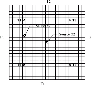
The previous developments are here applied to the IHCP proposed in [35]. It consist in identifying two heat source strengths in a long bar of squared cross section (50 × 50 mm) from temperature measurements at four different points. Figure 1 shows the temperature sensors location (T1, T2, T3 and T4) and the heat sources position (G1 and G2). The direct problem is defined by the following equations

with , and . The finite volume method has been used for spatial discretisation of the equations above. The resulting state-space model includes 529 ordinary differential equations, 3 input variables (the ambient temperature and the intensity of the heat sources G1 and G2) and 4 output variables (the temperature at the points were the sensors T1 to T4 are placed).

FIGURE 1 Scheme of the bar cross section. Discretisation grid. Sensors and sources location.

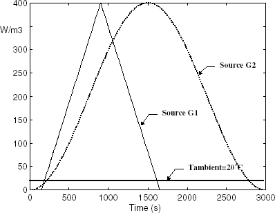
As measurements for the inverse problem, simulations coming from the direct model will be used. The ambient temperature is assumed to be constant and the intensity of the heat sources is a triangular (G1 source) or a sinusoidal (G2 source) function of time as shown in Fig. 2.

FIGURE 2 Input signals for simulations: heat sources intensity and ambient temperature.

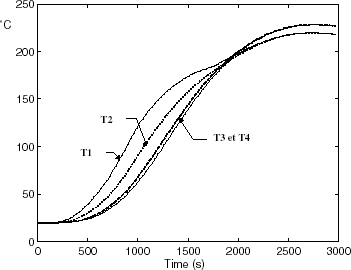
The initial temperature of the bar is assumed to be homogeneous and equal to 20°C. The direct simulation is performed over 100 time steps of 30 s. Figure 3 includes the time evolution of the bar response at points T1–T4.

FIGURE 3 Thermal response of the bar at points T1–T4.

IHCP with Free-noise Measurements

We firstly assume free-noise measurements. As indicated before, the inversion is based on the minimisation of the following criterion

where e(t) [] represents the difference between measurements and simulations, and Z(t) [] is the vector of unknown solicitations, the intensity of the sources G1 and G2 in the example. Q [] and R [] are assumed to be identity matrices. The regularisation parameter μ is chosen so that the estimations bias was as low as possible. μ values in the interval [, ] are considered. For each value, the evolution of the sources intensity is estimated by time integration of the full-order inverse model (21) and the standard deviation of the difference between the estimations and the actual intensity values (bias) is then calculated. Figure 4 includes the achieved results. It shows that the μ value leading to a minimal bias (1.3 W m⁻³ for the source G1 and 1.28 W m⁻³ for G2) is . The inversion results corresponding to such a μ value are given in Fig. 5. It can be seen that estimations and actual heat source intensity values are indistinguishable.

FIGURE 4 Noise-free measurements case. Inversion algorithm setting results. Regularising parameter value vs. estimations bias.

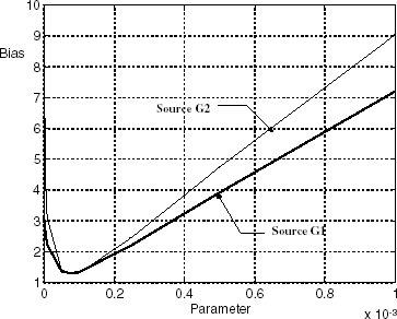
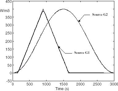
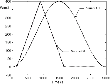
FIGURE 5 Inversion results achieved from the full-order model (μ = 0.75 × 10⁻⁴). Intensity of the heat sources: estimations (dotted line) and actual values (continuous line).

The inversion is now performed using reduction techniques. Two different approaches are considered:

1. Direct model size reduction (DMSR). Inversion then involves: (1) calculation of the full-order direct problem; (2) size reduction of the direct model; (3) inverse model calculation from the previous reduced-order model; and (4) time integration of the approached inverse model (31).

2. Inverse model size reduction (IMSR). Inversion is now carried out by: (1) calculation of the full-order direct problem; (2) inverse model calculation from the previous direct model; (3) size reduction of the inverse model (21); and (4) time integration of the reduced-order inverse model.

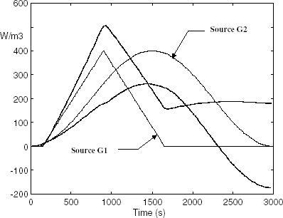
In both cases, involved state-variable models are reduced by the Moore’s method [31] described in the previous section. The results achieved for different reduction orders are included in Tables I and II. The values in columns 2 and 3 represent the standard deviation of the residuals (differences between the actual values and the estimations of the intensity sources). It can be seen that reduced direct models up to order 10 are useless for inversion purposes. On the contrary, the results achieved when reducing the inverse model at order 6 (6 ordinary differential equations) are as accurate as those from the full-order model (529 ordinary differential equations).

TABLE I. Reduced direct model. Standard deviation of the residuals

Order	Direct model
Source G1	Source G2
5	700.8342	682.7709
6	168.1725	163.7206
7	23.5605	23.0130
8	3.1493	2.9947
9	2.8961	2.7284
10	1.4488	1.2251
11	1.3862	1.7285
12	1.4491	1.8078
13	1.3157	1.2996
14	1.3123	1.3031
15	1.4742	1.2977

TABLE II Reduced inverse model. Standard deviation of the residuals

Order	Inverse model
Source G1	Source G2
5	1.7658	1.6846
6	1.1373	1.5258
7	1.2240	1.3123
8	1.3719	1.2441
9	1.3780	1.2143
10	1.3028	1.2884
11	1.3189	1.2670
12	1.3145	1.2704
13	1.3059	1.2790
14	1.3039	1.2829
15	1.3004	1.2840

Figures 6 and 7 show the intensity sources estimations coming from 6-order reduced models. The results achieved by IMRS are excellent (Fig. 6); on the contrary, those from DMRS (Fig. 7) are inadequate. To get similar high quality results by DMRS a 13-order reduced direct model is required.

FIGURE 6 Results from the inversion using a reduced model of order 6 (inverse model reduction).

FIGURE 7 Results from the inversion using a reduced model of order 6 (direct model reduction).

IHCP with Noise-disturbed Measurements

The same inverse problem is now solved using disturbed measurements. White noises with zero mean and standard deviation have been added to the previous “measurements” (simulations of the temperature evolution at points T1–T4). Such a formulation leads to random errors at 99% reliance in the range (poor quality data). 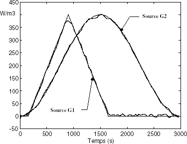The value of the regularisation parameter leading to a minimal standard deviation of the residuals is now (see Fig. 8), and the corresponding inversion results are shown in Fig. 9 (no reduction techniques have been used). As expected, the standard deviation of the difference between the sources intensity estimations and the actual values is greater than in the free-noise case: 4.5 W m⁻³ for the source G1 and 3.7 W m⁻³ for the source G2.

FIGURE 8 Noisy measurements case. Inversion algorithm setting using the full-order model. Standard deviation of the difference between actual sources intensity and estimations vs. regularisation parameter values.

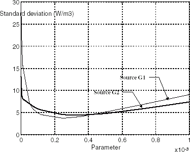
FIGURE 9 Inversion results achieved from the full-order model (μ = 2.5 × 10⁻⁴ and noise corrupted measurements). Intensity of the heat sources: estimations (dotted line) and actual values (continuous line).

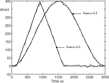
The full-order inverse model has been now reduced to the order 4. As shown in Figs. 9 and 10, no significant differences are observed between the accuracy of the estimations obtained from time integration of the full-order inverse model and those coming from the 4-order inverse model. The standard deviations of the differences between the actual values of the sources intensity and the estimations are now 4.2 W m⁻³ for the source G1 and 3.9 W m⁻³ for the source G2. The requirements concerning the inverse model quality decrease with increasing measurements noise.

FIGURE 10 Results from the inversion using a reduced model of order 4 (inverse model reduction and noise corrupted measurements): estimations (dotted line), actual values (continuous line).

Summary and Conclusion

This article is concerned with IHCP involving large-scale linear systems with unknown heat sources or boundary conditions. The IHCP is stated as an optimisation problem with a zero-order Tikhonov regularised objective functional. Numerical solution of this problem is usually obtained by iterative search algorithms as the conjugate gradient method. Each iteration involves time integration of three sets of partial differential equations, the so-called direct, adjoint and sensitivity problems. Such procedure can be applied very generally; however, the generality comes at the expense of computational and programming burdens. The computational efficiency of the Tikhonov regularisation method has been improved in this article via both Lagrange theory for dynamic optimisation and model reduction techniques.

First, we have proven that, for linear systems, the solution of the IHCP can be obtained by simple time integration of the so-called inverse model. It is a state-variable model of dimension which is analytically obtained from the direct and adjoint problems. Inputs variables to the inverse model are the temperature measurements, and its outputs variables are the unknowns we are looking for. Neither iterations nor sensitivity problem integration are hence required.

Afterwards, we have shown that the number of differential equations involved in the IHCP can be strongly reduced without a significant loss of accuracy in the estimations. This is specially interesting for large-scale (i.e. multidimensional) IHCP solving. Two different ways of applying reduction techniques to the IHCP have been proposed and tested. First one consist in size reduction of the direct problem. The resulting reduced order model is then used to calculate the inverse model whose time integration leads to the IHCP solution. In the second one, reduction techniques are directly applied to the full-order inverse model. Due to the special characteristics of it (two boundary-value problem) a modified reduction technique has been proposed. From a numerical point of view, the first way of applying reduction techniques to the IHCP is more efficient as it requires less computing time. However, the second one is more accurate. In other words, it allows more significant reduction rates for the same accuracy.

A numerical example (estimation of 2 heat sources strengths in a 2D solid body) has been used to show the performances of our proposals. The corresponding direct problem involves 529 ordinary differential equations. As it was expected, excellent results are obtained from time integration of the full-order inverse model. Estimations and actual values of the heat sources intensity are indistinguishable. It must be noticed that the Lagrange theory supplies a different way for numerical solution of the IHCP, it does not introduce essential modifications in the Tikhonov regularisation method. Concerning IHCP reduction, this example shows that excellent results are also obtained by time integration of very low dimension inverse models (4–6 ordinary differential equations, instead of 529). The computing time required for inversion is strongly reduced without a significant loss of accuracy. In general, reduction techniques are all the more effective as the dimension of the direct problem is large and the experiment is long.

Future works in the framework of large-scale IHCP will be focused in on-line estimations which involve incorporation of sequential concepts to the inverse model solving.

Nomenclature

Table

A	=	state matrix () in the state-space direct model
B	=	command matrix in the equivalent state-space direct model
c(M)	=	heat capacity at point M
E	=	command matrix in the state-space direct model
F	=	state matrix () in the equivalent state-space direct model
	=	convective coefficient at point M
	=	thermal conductivity at point M
K(t)	=	Kalman gain matrix
K∞	=	Kalman gain matrix for infinite horizon problems
O	=	output matrix in the equivalent state-space direct model
P	=	similar transformation matrix
Q	=	residuals weighting matrix
R	=	unknown weighting matrix
S(t)	=	defined by Eq. (19)
S∞	=	as S(t), but for infinite horizon problems
T(M, t)	=	thermal field
	=	vector of temperature at the nodes of the discretisation mesh
	=	vector of temperature measurements
T∞ (M, t)	=	environment temperature field
	=	controllability gramian
	=	observability gramian
Z(M, t)	=	field of the problem unknowns
Z(t)	=	vector of the problem unknowns

Greek Symbols

Table

α(M)	=	residuals weighting function
β(M)	=	unknown weighting function
ϕ(M, t)	=	prescribed heat density flux
	=	adjoint temperature field
	=	co-state vector
μ	=	regularisation parameter
σ(M, t)	=	field of heat sources or sinks intensity
Ω	=	system domain
∂Ω	=	system frontier
ψ(M, t)	=	solicitations field

Special Symbols

Table

	=	boundary conditions operator
	=	spatial heat operator
	=	objective functional

Annex

Proof 1: The Necessary Conditions for a Minimum

Using Leibniz’s rule and taking into account that t_o and t_f are fixed and known, the increment in (see Eq. (6)) as a function of the increments in T, , Z and t is:

where represents the increment of the derivative of T with respect to the time. To eliminate it in Eq. (A.1), we integrate by parts as follows

where for is fixed and known.

The minimum of is achieved when for all independent increments in its arguments. Setting to zero the coefficients of the independent increments , , and , after substitution of Eq. (A.2) into Eq. (A.1), yields to the following necessary conditions for a minimum:

Proof 2: Sweep Method

To solve the problem specified by Eq. (15) we shall use the sweep method proposed in [28]. Thus, assume that T(t) and satisfy the following relationship

for all for some as yet unknown matrix function S(t) and vector function v(t). If we can find such S(t) and v(t), then the assumption is valid. Introducing the co-state expression (A.3) in Eq. (15) we get

and

Since the Eq. (A.5) holds for all state trajectories given any , it follows that

with . The unknowns we are looking for are then given by

Proof 3: Block-diagonal Transformation

It can be easily verified that the inverse of the transformation T (see Eq. (32)) is

Hence, applying transformation T on Eq. (21) leads to the state matrix:

So, the necessary and sufficient condition for a block-diagonal state matrix is given by

Balanced Realisation

Assuming eigenvalues of the state matrix F in model (23) to be strictly in the left half-plane, then we can define the controllability gramian and the observability gramian of model (23) as:

respectively. By considering the corresponding matrix differential equations it is easily verified that and satisfy the following Lyapunov equations (cf. [36]):

Both and are definite positive matrices of dimension []. It is easily demonstrated that they depend on the state-space co-ordinates. If it is changed to for some non-singular P, the controllability and observability gramians become:

A balanced realisation is obtained for a matrix P which verifies the following equation:

where is a diagonal matrix containing the Hankel singular values of the system. Such transformation may be obtained by the method proposed by Laub [37], which is one of the most efficient ones. The matrix is first decomposed as (Cholesky factorisation method):

The product is then a definite positive matrix. It can be transformed in a diagonal matrix by solving the following symmetric eigenvalues problem:

The matrix P we are looking for is given by (see [37] for demonstrations):

References

- Beck J.V. Blackwell B. C.R. St-Clair Jr. 1985 Inverse Heat Conduction: Ill-Posed Problems Wiley Intersciences New York
- Alifanov O.M. 1994 Inverse Heat Transfer Problems Springer-Verlag Berlin Heidelberg
- Dinh N.H. 1998 Methods for Inverse Heat Conduction Problems Peter Lang Frankfurt
- Hadamard J. 1923 Lecture on Cauchy’s Problem in Linear Partial Differential Equations Yale University Press London
- Beck J.V. 1962 Calculation of surface heat flux from an internal temperature history ASME Paper 62-HT-46
- Murio D.A. 1993 The Mollification Method and the Numerical Solution of Ill-posed Problems Wiley Intersciences New York
- Tikhonov A.N. Arsenin V.Y. 1977 Solutions of Ill-posed Problems V.H. Winston Washington DC
- Alifanov , O.M. 1974 . Solution of an inverse problem of heat conduction by iteration methods . J. Engng. Phys. , 26 ( 4 ) : 471 – 476 .
- Alifanov , O.M. and Artyukhin , E.A. 1975 . Regularized numerical solution of nonlinear inverse heat conduction problem . J. Engng. Phys. , 29 ( 1 ) : 934 – 938 .
- Alifanov , O.M. and Rumyantev , S.V. 1978 . One method of solving incorrectly stated problems . J. Engng. Phys. , 34 ( 2 ) : 328 – 331 .
- Rumyantev , S.V. 1986 . Ways of allowing for a priory information in regularizing gradient algorithms . J. Engng. Phys. , 49 ( 3 ) : 932 – 936 .
- Alifanov , O.M. and Rumyantev , S.V. 1987 . Application of iterative regularization for the solution of incorrect inverse problems . J. Engng. Phys. , 53 ( 5 ) : 1335 – 1342 .
- Jarny , Y. , Özişik , M.N. and Bardon , J.P. 1991 . A general optimization method using adjoint equation for solving multidimensional inverse heat conduction . Int. J. Heat Mass Transfer , 34 ( 11 ) : 2911 – 2919 .
- Huang , C.H. and Özişik , M.N. 1992 . Inverse problem of determining unknown wall heatflux in laminar flow through a parallel plate duct . Num. Heat Transfer A , 21 : 55 – 70 .
- Scheuing , J.E. and Tortorelli , D.A. 1996 . Inverse heat conduction problem solution via second-order design sensitivities and Newton’s method . Inverse Problems in Engineering , 2 : 227 – 262 .
- Dorai , G.A. and Tortorelli , D.A. 1997 . Transient inverse heat conduction problem solutions via Newton’s method . Int. J. Heat Mass Transfer , 40 ( 17 ) : 4115 – 4127 .
- Prud’homme , M. and Nguyen , T.H. 1997 . Whole time-domain approach to the inverse natural convection problem . Num. Heat Transfer A , 32 : 169 – 186 .
- Huang , C. and Chen , W. 1999 . A three dimensional forced convection problem in estimation surface heat flux by conjugate gradient . Int. J. Heat Mass Transfer , 42 : 3387 – 3403 .
- Prud’homme , M. and Nguyen , T.H. 1999 . Fourier analysis of conjugate gradient method applied to inverse heat conduction problems . Int. J. Heat Mass Transfer , 42 : 4447 – 4460 .
- Huang , C. and Wang , S. 2000 . A three dimensional forced convection problem in estimation surface heat conduction problem in estimating heat flux by conjugate gradient . Int. J. Heat Mass Transfer , 43 : 3171 – 3181 .
- Khachfe , R.A. and Jarny , Y. 2000 . Numerical solution of 2-D nonlinear inverse heat conduction problems using finite-elements techniques . Num. Heat Transfer , 37 ( 1 ) : 45 – 67 .
- Khachfe , R.A. and Jarny , Y. 2001 . Determination of heat sources and heat transfer coefficient for two-dimensional heat flow – numerical and experimental study . Int. J. Heat Mass Transfer , 44 : 1309 – 1322 .
- Petit D. Peruzzi S. 1996 Régularisation d’un problème inverse en conduction par utilisation d’un modèle réduit identifié In: Proceedings Congrès SFT 96
- Petit D. Videcoq E. Sadat H. 1998 Resolution of inverse heat conduction problem with a reduced model In: Proceedings of Int. Heat Transfer Conference 98
- Battaglia J.L. Neveu A. 1998 Identification du flux de chaleur dans un essai de tribologie. Utilisation d’un modèle réduit In: Proceedings of SFT’98, Thermique et Environnement
- Gafsi A. Lefebvre G. Palomo E. 2000 Réduction et inversion d’un modèle de système thermique complexe: détermination d’une sollicitation inconnue appliquée à un bâtiment In: Proceedings of Congrès français de thermique – SFT 2000
- Lewis F.L. 1986 Optimal Control John Wiley & Sons New York
- Bryson A.E. Ho Y.C. 1975 Applied Optimal Control. Hemisphere New York
- Palomo E. 2000 Résolution de problèmes thermiques de grande dimension. Méthodes de réduction, Habilitation à Diriger des Recherches Université Paris 12
- Mikhailov M.D. Özişik M.N. 1984 Unified Analysis and Solutions of Heat and Mass Diffusion Dover Publications, Inc. New York
- Moore B.C. 1981 Principal components analysis in linear systems: controlability, observability and model reduction IEE Transactions on Automatic Control AC 26 1 17 32
- Marshall , S.A. 1966 . An approximate method for reducing the order of a linear system . Control , 10 : 642 – 643 .
- Glover , K. 1984 . All optimal Hankel-norm approximations of linear multivariable systems and their L∞-error bounds . Int. J. Control , 39 ( 6 ) : 1115 – 1193 .
- Bartels , R.H. and Stewart , G.W. 1972 . Solution of the matrix equation AX + XB = C . Comm. ACM , 15 : 820 – 826 .
- Le Niliot , C. 1998 . The boundary-element method for the time-varying strength estimation of point heat sources: application to a two-dimensional diffusion system . Numerical Heat Tranfer, Part B , 33 : 301 – 321 .
- Arnold L. 1971 Stochastic Differential Equations: Theory and Applications John Wiley & Sons New York
- Laub A.J. 1980 Computation of balancing transformation In: Proceedings of 1980 Joint Automatic Control Conference San Francisco California FA8-E