Identifying Counter-Gradient term in atmospheric convective boundary layer

Abstract

Since Deardoff [5] derived the counter-gradient term contribution, a good representation has been searched for this term. An inverse problem methodology is used to identify this property. The inverse analysis is performed minimizing an objective function: the square difference between experimental and model data added to a regularization function. Two regularization functions are used: second-order maximum entropy, and Tikhonov regularization of second-order. The scheme is tested with synthetic noise data. A new formulation for the counter-gradient is also presented.

Keywords:

• Counter-gradient term estimation
• Inverse problems
• Meteorological models

1 Introduction

Terms denoting the turbulence can be represented by Reynolds fluxes. The process to parameterize the Reynolds tensors is called the closure problem. In the first order closure, turbulent fluxes are given by the product between the gradient of the mean quantity and an eddy diffusivity. A new formulation for first order closure is constituted considering the contribution of the counter-gradient term. Since Deardorff [5] has derived an expression for counter-gradient term, also performing some experimental procedure to identify this term, intense research has been done. Turbulence is always present in the Planetary Boundary Layer (PBL), where several stability conditions are found: convective, neutral, and stable. For convective conditions, the largest transporting eddies may have a similar size as the boundary layer height itself and, in particular, the flux can be in the opposite direction of the local gradient of the mean quantity. For neutral and stable conditions, the flux of a quantity is proportional to the local gradient of that quantity. In fact, the counter-gradient represents nonlocal influences on the mixing by turbulence, and as this term is small in stable conditions it is, therefore, neglected in these conditions [12].

Holtslag and Moeng [11] (HM91) derived a counter-gradient term from turbulent heat flux, and their parameterization for the transport term is based on the results from large eddy simulation (LES). Cuijpers and Holtslag [4] (CH98) generalized the expression of the HM91 by writing the nonlocal term as a function of vertical velocity variance and an integral form for the flux.

The purpose of this article is two fold. Firstly, a new approach to counter-gradient term is introduced. The new formulation is based on the parameterization presented in [4]; however the convective scale for a scalar is a space average of the mean quantity inside of the PBL – additionally, the mixing length is computed by Taylor's theory [7]. Secondly, the counter-gradient term is identified by numerical procedures, from experimental data, based on an inverse problem methodology.

An implicit inversion technique is used for determining the counter-gradient term by a numerical scheme. The inverse problem is formulated as an optimization problem, where the objective function is defined as the least-squares fit between model results and experimental data. A stabilizer (or regularization) operator is added to the objective function with the help of a Lagrange multiplier (also called regularization parameter). Iteration proceeds until objective function converges to a specified limit value. Synthetic data with Gaussian white noise corruption are used to simulate experimental data.

2 New Approach for the Counter-gradient Term

The first order closure approach considering the counter-gradient term can be expressed as

where is the vertical turbulent Reynolds flux, k _zz is vertical eddy diffusivity, γ _χ is the counter-gradient term, w is the vertical component of the velocity of wind, and χ is mean quantity (mass or temperature).

Cuijpers and Holtslag [4] have presented an expression for the counter-gradient, given by

h being the PBL height, is the velocity variance, w _* is the convective scale for velocity, b is a constant and χ _* is a scale for mean quantity:

Combining Eqs. (1)–(3) an integral equation is resulted for the turbulent flux . One procedure to avoid this difficulty is to consider the counter-gradient term as zero in the first step of the time integration, and after that, having an estimative for the turbulent flux, the Reynolds fluxes can be computed from Eqs. (1) and (2) using the flux previously computed [13]. In order to circumvent this constraint in the first step of time integration, a new formulation for convective scale χ _* is proposed. In the new formulation χ _* is given by

The constant b in Eq. (2) in [4] is 1.5, whereas in the new formulation this constant is b = 0.07.

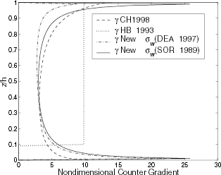
There are many expressions for the velocity variance , see [7,11,18] and Appendix. Different approaches for the counter-gradient term are displayed in Fig. 1, the Holtslag and Boville's [12], (HB-93) parameterization is also shown.

FIGURE 1 Different parameterizations for the nondimensional counter-gradient.

3 Estimation of Counter-gradient Term by Numerical ProcEdures

As pointed out in [3], fully computational methods can be used to estimate some properties in turbulent flux. In particular, it is suggested that an inverse analysis could also be a good strategy to identify the counter-gradient term.

To exemplify the inverse methodology, the scheme is illustrated considering a one-dimensional pollutant dispersion model. The diffusion of passive scalars is given by mass conservation principle. A special case occurs in the dispersion of the instantaneous area sources. In this case, the diffusion equation can be simplified to

with following initial and boundary conditions

where is the mean concentration to be measured, K _zz is the vertical eddy, γ _c is the counter-gradient term to be estimated, and h is the height of the atmospheric boundary layer. Our numerical model consists of Eq. (5) numerically solved by central finite difference method of second order O(Δ z ²) in space and the explicit Euler method in time. The approximate solution is denoted by .

3.1 Inverse Model

In order to establish the inverse analysis, it is assumed that measurements are available at i = 0,1,…,N _z vertical points, and at n = 1,2,…,N _t time steps. The vector γ = γ (z _i )| i = 0,1,…,N _z -1) denotes the discrete counter-gradient term to be obtained by a nonlinear constrained minimization problem:

where the objective function is given by

with Ω being a regularization function and λ a positive parameter, called Lagrange multiplier. The bounds l _i and u _i are chosen to allow the inversion to lie within some physical limits. The least square difference between experimental data and the calculated values is represented by

The regularization operator can be expressed by Tikhonov scheme [20] as

here γ ^(m) denotes the mth difference. In general the parameter κ _m,j is chosen as κ _m,j = δ _m,j (Kronecker delta) and the regularization is named Tikhonov – j regularization operator, where j denotes the order of the regularization.

Another regularization technique is given by an entropic scheme [3,16,17]

with

and represents the mth difference among the parameter vector [2,17]. The function S ^m attain its global maximum when all s _q are the same, i.e., a uniform distribution with , in contrast, the lowest entropy value is reached when all elements s _q but one are set to zero. This scheme is based on Jaynes' criterium of inference [14], called maximum entropy principle (MaxEnt).

3.2 Optimization Algorithm

The optimization problem is iteratively solved by the quasinewtonian optimizer routine from the NAG Fortran Library [9], with variable metrics. This algorithm is designed to minimize an arbitrary smooth function subject to constraints (simple bound, linear or nonlinear constraints), using a sequential programming method.

This routine has been successfully used in several previous works: in geophysics, hydrologic optics, heat transfer, and meteorology.

4 Results for Counter-gradient Term Estimation

In order to verify the method presented in the previous section, some numerical experiments were performed. The use of synthetic data is a standard procedure to test a methodology in inverse problems, emulating experimental data. Therefore, the synthetic data are obtained from a concentration computed in the forward problem added to a random fluctuation.

The expression for the eddy diffusivities in the diffusion Eq. (5) is given by [7]

where w _* is the convective scale for velocity, h is height of the atmospheric boundary layer, and Ψ = 0.913 is the nondimensional dissipation function, as computed by Degrazia [8].

In all simulations the following discretizations were Δ z = 10 m with N _z = 100, and Δ t = 0.4 s with N _t = 1000; and γ (z) = 0 is assumed as initial guess. For meteorological parameters the following values were used: h = 1000 m; ; (friction velocity).

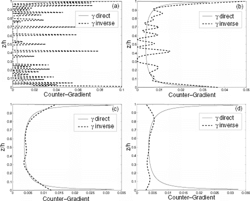
For the estimation of the counter-gradient term three levels of noise were used: 1, 2.5, and 5%. The best results were obtained with second order regularization operator, for Tikhonov and entropic regularization. The reconstruction using Tikhonov-2 and MaxEnt-2 were similar. In this article only inversions with MaxEnt-2 are shown. Figure 2> shows the inversion for different levels of noise. As expected, by increasing the level of noise the inversion become poorer. The numerical values for regularization parameters are: 2.5 × 10¹⁰ for 1% of noise, 4.5 × 10¹⁰ for 2.5% of noise, and 4× 10¹⁰ for 5% of noise. As expected, the reconstruction is degraded as the level of noise enhances.

FIGURE 2 New counter-gradient estimation by second-order maximum entropy with given in [18]: (a) noise 1%, with λ = 2.5×10¹⁰; (b) noise 2.5%, with λ = 4.5× 10¹⁰; and (c) noise 5%, with λ = 4.0×10¹⁰.

In order to make clear the role of regularization parameters, Fig. 3 shows the estimation for three different λ Clearly, as λ → 0 some spurious solutions (oscillations) appear in the inversion (Fig. 3a), even for small values of λ (Fig. 3b), for λ → ∞ the optimization is only focused on the regularization term (see Fig. 3d). Good inversions are obtained with appropriate values for λ , as shown in Fig. 3c. An important feature is a good choice of the regularization parameter.

FIGURE 3 Influence of the regularization parameter to 1% of noise: (a) without regularization; (b) λ = 1.0 × 10⁷ (c) λ = 2.5 × 10¹⁰; (d) λ = 1.29 × 10¹¹.

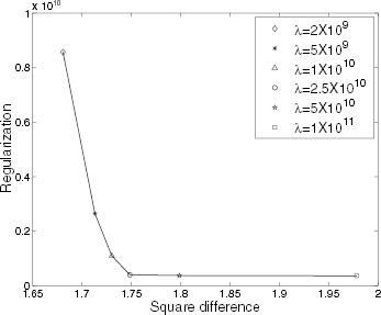
Many schemes have been proposed to find the value of the regularization parameter which gives a fine balance between square difference and regularization term. Some of these techniques are: Morozov's discrepancy principle [1, 15], the L-curve and the generalized cross validation [1]. Here, the Hansen's procedure [10], essentially the maximum curvature of the L-curve, was used producing good results. Figure 4 displays the L-curve for different Lagrange multipliers, for estimation with 1% of noise. From the plot it can be seen that λ ≈2.5 × 10¹⁰ is a good choice.

FIGURE 4 L-curve for reconstruction of counter-gradient with 1% of noise.

5 Performance of the Counter-Gradient Formulation

The forward problem described by Eqs. (5) and (6) was also used to verify the behavior of the new counter-gradient approach given by expressions (2) and (4).

It is worth noting that there is a small difference when the concentration is computed from counter-gradient in which χ _* is given by Eq. (3) or when the counter-gradient is calculated by Eq. (4). In our simulation, the variance of the vertical velocity appearing in formula (2) is that calculated according to Degrazia et al. [7], from analytical integration of the spectrum of kinetic energy. Other formulas for the variance are shown in the Appendix.

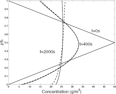
Figure 5 shows the simulation of the diffusion with and without the presence of the counter-gradient correction. If there is no transport in the counter-gradient direction, the PBL will be homogeneous in a shorter period of time than when the counter-gradient contribution is present in the process. Figure 6 displays the concentration profile at two times, using the Cuijpers–Holtslag's approach Eqs. (2) and (3), with σ _w given by Eq. (A.2) and the counter-gradient term proposed here — Eqs. (2) and (4), with σ _w given by Eq. (A.3). A small difference is seen from Fig. 6.

FIGURE 5 Concentration profiles at three times t = 0 s, t = 400 s and t = 2000 s: the solid line represents the diffusion without counter-gradient term, the dashed line represents the use of counter-gradient term given by Eqs. (2), (4) and (A.3).

FIGURE 6 Concentration profiles for three time periods: the solid line with counter-gradient term given by Eqs. (2), (4) and (A.3); the dashed line the counter-gradient is given in [4] (Eqs. (2), (3) and (A.2)).

6 Conclusion

The methodology proposed for estimating the counter-gradient term was effective to proceed nice reconstructions of this function. Good results were obtained even for a high level of noise with second order Tikhonov regularization and second-order maximum entropy principle, showing that the inverse model is robust related to the noise in experimental data. The determination of the regularization parameter by L-curve, following the procedure presented by Hansen [10], permitted to find out an appropriated value for both regularization operators.

The determination of turbulent properties by inverse procedure from available experimental data is useful under situations out of the scope of the theoretical assumptions, e.g., sometimes flat terrain hypothesis is assumed to derive some property; therefore, such properties can be estimated on complex terrain by using inverse analysis. However, as can be verified in Tables I and II, the differences between exact and estimated values (Table II) – O(10^-4) – are of the same order of magnitude of the counter-gradient models (Table I) – O(10^-4). Therefore, the inverse technique cannot be used to select the best parameterization for the counter-gradient term.

TABLE I Difference between several formulations for the counter-gradient term

γModel	ρModel
γCH98	ρCH98=3.5 × 10^−4
γHB93	ρHB93=6.4 × 10^−3

TABLE II Square error between exact and estimated counter-gradient terms for several levels of noise

1% noise	2.5% noise	5 % noise
3.1 × 10^-5	7.5 × 10^-5	2.6 × 10^-4

The proposed modification for the counter-gradient in the Cuijpers–Holtslag's formulation [4] worked well, producing similar results of those obtained with CH-98 expression [4]. The CH-98's approach has been compared with experimental data [4], thus this is an indirect validation of our expression for the counter-gradient term. Therefore, the following formula for the counter-gradient term

can be used in operational air-pollutant dispersion models, as well as in meteorological simulators under convective condition for the planetary boundary layer.

Nomenclature

Table

b	=	constant in Eq. (2)
	=	mean concentration (g m^−3)
C i,n	=	approximated solution for concentration
h	=	boundary layer height (m)
J(γ)	=	objective function
K zz	=	vertical eddy diffusivity (m^2 s^−1)
R(γ)	=	square difference term
S(γ)	=	entropy regularization function
u *	=	friction velocity (m s^−1)
w	=	wind vertical component (m s^−1)
w *	=	convective scale for velocity (m s^−1)
	=	vertical turbulent flux of quantity
γ	=	counter-gradient term (g m^−2 s^−1)
λ	=	regularization parameter
	=	variance of the vertical velocity (m^2 s^−1)
χ *	=	scale for mean quantity (g m^−3)
Δ t	=	time discretization (s)
Δ z	=	vertical space discretization (m)
Ψ	=	nondimensional dissipation function
Ω (γ)	=	general regularization function

Appendix A

Vertical Velocity Variance Parameterizations

Expressions for velocity variance in convective boundary layer (CBL) are provided in this section. These values are used to compute the counter-gradient term given by Eq. (2). Table I shows the difference between the counter-gradient term evaluated by several variance expressions.

Sorbjan [18] (page 113), (SOR89): Using D = 0 ,c _wt = 0.5 ,c _wb = 1 and R = −0.2

Holtslag and Moeng [11] for CBL (HM 91):

Degrazia et al. [6] for CBL [7] (DEA 97)

where c _i = 0.3 for u-component and 0.4 for v, w components, , spectral peak frequency in neutral stratification, is the model spectral peak. The stability function q _i is given by:

References

- Bertero M Boccacci P 1999 Introduction to Inverse Problems in Imaging, Institute of Physics
- de Campos Velho HF Holtslag AAM Degrazia GA Pielke RA 1998 New parameterizations in RAMS for vertical turbulent fluxes Technical Report, Department of Atmospheric Sciences, Colorado State University Fort Collins (CO) USA
- de Campos Velho , HF , de Moraes , MR , Ramos , FM , Degrazia , GA and Anfossi , D . 2000 . An automatic methodology for estimating eddy diffusivity from experimental data . Nuovo Cimento , 23-C : 65
- Cuijpers , JWM and Holtslag , AAM . 1998 . Impact of skewness and nonlocal effects on scalar and boundancy fluxes in convective boundary layers . J. Atmos. Sci , 55 : 151
- Deardorff , JW . 1966 . The countergradient heat flux in the lower atmosphere and in the laboratory . J. Atmos. Sci , 23 : 503
- Degrazia , GA and Moraes , OLL . 1992 . New model for eddy diffusivity in a stable boundary layer . Boundary Layer Meteorol , 58 : 205
- Degrazia , GA , de Campos Velho , HF and Carvalho , JC . 1997 . Nonlocal exchange coefficients for the convective boundary layer derived from spectral properties . Beitr. Phys. Atmos , 70 : 57
- Degrazia , GA . 1998 . Modelling dispersion from elevated sources in a planetary boundary layer dominated by moderate convection . Nuovo Ciment , 21C : 345
- E04UCF routine 1995 NAG Fortran Library Mark 17 Oxford UK
- Hansen , PC . 1992 . Analysis of discrete ill-posed problems by means of the L-curve . SIAM Rev. , 34 : 561
- Holtslag , AAM and Moeng , CH . 1991 . Eddy diffusivity and countergradient transport in the convective boundary layer . J. Atmos. Sci. , 48 : 1690
- Holtslag , AAM and Boville , BA . 1993 . Local versus nonlocal boundary layer diffusion in a global climate model . J. Climate , 6 : 1825
- Holtslag AAM 1998 Personal communication
- Jaynes , ET . 1957 . Information theory and statistical mechanics . Phys. Rev , 106 : 620
- Morozov , VA . 1966 . On the solution of functional equations by the method of regularization . Soviet Math. Dokl , 7 : 414
- Muniz , WB , Ramos , FM and de Campos Velho , HF . 2000 . Entropy and Tikhonov-based regularization techniques applied to the backwards heat equation . Comp. Math. Appl. , 40 : 1071
- Ramos , FM , de Campos Velho , HF , Carvalho , JC and Ferreira , NJ . 1999 . Novel approaches on entropic regularization . Inverse Probl. , 15 : 1139
- Sorbjan Z 1989 Structure of the Atmospheric Boundary Layer, Prentice Hall
- Taylor , GI . 1921 . Diffusion by Continuous Movements . Proc. London Math. Soc. , 20 : 196
- Tikhonov AN Arsenin VI 1977 Solutions of Ill-posed Problems, John Wiley & Sons