Computation of magnetic field sources from measurements using iterative regularization

Abstract

This article deals with the solution of inverse problems in magnetostatics. The cases the authors have considered are related to the determination of the current density or positions of air coils on the basis of magnetic field measurements. These problems are ill-posed, so regularization techniques are needed. The authors discuss the main iterative regularization principles and D-optimal experimental design. Numerical and experimental results are presented.

Keywords:

• Iterative regularization
• Inverse problem
• Magnetostatics

Introduction

In superconducting magnet technology, coils are located in cryostatic equipment. Therefore, a numerical tool calculating the coil parameters from magnetic field measurement is interesting for faulty operating conditions determination. This leads us to solve two different inverse problems: a linear inverse problem to compute the current densities on the basis of field measurements, and a nonlinear inverse problem for the computation of the coil positions. In solving these problems, an experimental design is to be chosen.

Several aspects of electromagnetism raise inverse problems. Inverse problems for Maxwell equations in general have been discussed in [1]. Magnetostatic inverse problems in the field of biomagnetism have been discussed by several authors. Reference [2] gives an overview of the different methods used to solve these problems. Reference [3] studies the identification of the plasma magnetic contour from external measurement by means of equivalent currents, leading to a linear inverse problem whose formulation is similar to our problem. The authors employ the Truncated Singular Value Decomposition to solve it. In the case of superconducting magnet diagnosis, the subject has only been discussed in [4] where the Levenberg–Marquard algorithm was used. In this reference, the authors obtain indications on coil positions. To our knowledge, the computation of an experimental design has not been performed in magnetostatic inverse problems.

In this article, the authors present a different approach to solve the inverse problems. This approach is based on iterative regularization [5,6] that has been chosen because it can be easily applied to both linear and nonlinear problems. We reconstruct the current densities or the coil axial positions of Magnetic Resonance Imaging (MRI) magnets. For the linear inverse problems, a D-optimal experimental design is computed in order to improve the accuracy of the solutions. The main contribution of this article is the experimental validation of the methods presented in [7,8] where only numerical tests were performed.

The first part of this article deals with a general presentation of the problem under analysis. The second part outlines the solution of the linear inverse problem. Numerical and experimental results are presented; a D-optimal experimental design is calculated. The third part describes the solution of the nonlinear inverse problem with numerical and experimental results.

General Presentation

Description of MRI Magnets

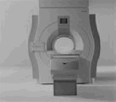
The magnets we consider are magnets for MRI. These magnets produce a high and uniform magnetic field in a Volume Of Interest (VOI), which is a sphere at the center of the magnet. Typically, the field values range from 0.5 to 1.5 T and the field homogeneity is 10 ppm (part per million). To create such a strong magnetic field, superconducting technology is required. Therefore the magnet coils are made of superconducting wire and the whole magnet is placed in a cryostat. The magnet length is about 1.5 m and the bore diameter 0.9 m (Fig. 1). The field homogeneity is checked by performing measurements at the surface of the VOI. In operating conditions, when the field homogeneity does not comply with the specifications, there is no access to the coils inside the cryostat. Thus, a numerical tool to compute the coil parameters from the magnetic field values is interesting. A common problem encountered in operation is the axial displacement of one of the coils.

FIGURE 1 Example of a MRI magnet.

Magnetostatics Equations

We assume that the magnetic field is static and that the equipment is in vacuum. The Biot–Savart law gives the magnetic flux density B at the point P produced by a current distribution j at the point M [9]:

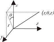
In a MRI magnet, the principal magnetic field is parallel to the magnet axis. Thus, we consider only the axial component of the field B _z . The system possesses cylindrical symmetry, the current density is only azimuthal (Fig. 2). In cylindrical coordinates (Fig. 3), the Biot – Savart law is expressed as follows:

where

FIGURE 2 Cross-section of the magnet geometry.

FIGURE 3 Cylindrical coordinates.

Inverse Problems Under Analysis

We will discuss two types of problems: a linear inverse problem where the coil geometry and positions are known, and we reconstruct the current density from measured magnetic field values, and a nonlinear inverse problem where the current density is known and the coil dimensions are reconstructed.

Linear Inverse Problem

Inverse Problem Statement

Computing the current density from magnetic field values leads us to solve a linear integral equation of Fredholm of the 1st kind. It has been demonstrated [10] that solving this type of equation is an ill-posed problem. We denote J the vector of all the densities. The spatial discretization and collocation of the Biot–Savart law (2) lead to a singular integral discretization that can be stated as the following matrix relation:

where B denotes the magnetic field values, and A is the matrix of the contributions of each coil to the field values at each point. Writing the normal equations for this problem leads to the relation:

In the problem under analysis, the matrix A ^T A is ill-conditioned. Therefore, we cannot compute the solution by direct computation of (5).

Solution

The authors use iterative regularization [5–7]. According to this method, the inverse problem is formulated as an optimization problem. It is solved by an iterative method coupled to a stopping rule. The number of iterations in the minimization is the regularization parameter.

Objective Function

The objective function to minimize is the quadratic residual R between the computed magnetic field and the measured field.

The direct problem i.e. A J is computed by integration of (2). The first two integrations are performed analytically while the last integration is computed numerically by a Gauss quadrature rule.

Minimization Procedure

The minimization is performed with the conjugate gradient method [11].

The residual gradient is calculated by:

where A _i denotes the ith column of the matrix A. The descent direction is computed by:

where D _k and G _k denote the descent direction and the gradient at iteration k. The descent parameter is calculated by making a one variable minimization along the descent direction D . As the problem is linear, this minimization has an analytical solution:

Choice of the Regularization Parameter

The authors employ two different ways to choose the regularization parameter.

Discrepancy Principle [ 5 ] The authors match the residual and the error level δ in the input data. We define the error level by:

Thus, the final iteration is determined when:

Practically, the exact error level is not known. So, in experimental cases, the authors compute an approximation of δ ² based on the accuracy of the measurement equipment.

L-curve [ 12 ] The L-curve method is positive because it does not require the error level to be known. The value of the residual is plotted versus the solution norm for different regularization parameters. This curve has an L-shape. The iteration number is chosen by selecting the value corresponding to the corner of the L.

Numerical Example

We consider a magnet (Fig. 4) divided into 24 coils. Our goal is to compute the current density values from 101 measurement points: 1 at the VOI center and 100 on the sphere.

FIGURE 4 Geometry of the numerical example.

The condition number of the matrix (A ^T A) is 10²³. Hence, the problem under analysis is unstable.

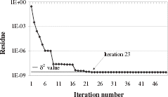
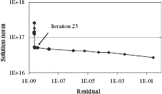
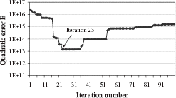
We have simulated experimental data by adding a gaussian random noise of 10 ppm to the exact data. For this noisy data, the exact value of δ² is 2.7×10⁻⁹. The minimization procedure starts with all values set at zero. The application of the discrepancy principle (Fig. 5) or the use of the L-Curve (Fig. 6) indicates the 23rd iteration as the final iteration to be selected.

FIGURE 5 Application of the discrepancy principle.

FIGURE 6 L-curve.

In order to check the optimality of this iteration number, we plot the quadratic error:

versus the iteration number. We observe that the error E decreases until the 23rd iteration then increases (Fig. 7). Therefore, the final iteration selected is the optimal iteration. By comparing the computed solution for 23 iterations with the exact solution, we observe a good agreement (Fig. 8). The maximum relative error of the estimated densities:

is 9%. At the end of the minimization, the computed solution becomes unstable (Fig. 9). Negative and positive oscillations around the exact values appear, computed values are several times higher than the exact values.

FIGURE 7 Quadratic error versus iteration number.

FIGURE 8 Exact and calculated solutions 23 iterations.

FIGURE 9 Exact solution and calculated solutions 500 iterations.

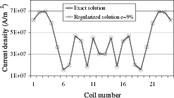
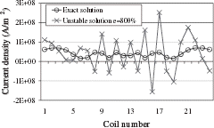
This numerical test shows that the proposed method enables us to find the current density with measured field values as input data.

Experimental Validation

The purpose of this experimental validation is to show the instability of real magnetostatic inverse problems and to test the proposed method on these problems.

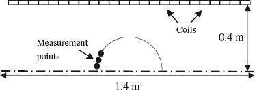
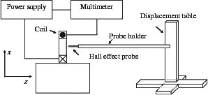
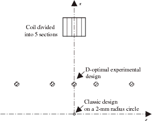
General Description of the Experiment We use resistive circular air coils of rectangular cross section to produce a magnetic field. This field is measured using a gaussmeter with a Hall-effect probe which is moved by displacement tables. The experimental scheme is shown in Fig. 10.

FIGURE 10 Experimental scheme.

The magnetic field produced in this experiment is much lower than the MRI field. However, we do not expect any large difference between resistive and superconducting coils concerning the application of the numerical methods because the magnetic field varies linearly with the current density.

Description of the Measurements The coil power supply is current controlled. Therefore, the current in the coil does not vary with the modification of the coil resistance with temperature. Current intensity is measured with a multimeter whose accuracy is 0.34% for the current used (2.8 A). The Hall-effect probe dimensions are 0.2 × 0.2 mm. For the measured field (about 10⁻² T), the gaussmeter has an absolute accuracy of 3×10⁻⁴ T. For each point, we perform 100 acquisitions of the field values and we take the mean value of these acquisitions. As a result, the variance of the measurement error is reduced by a factor of 10 [13]. The probe position is controlled by displacement tables. These tables have a positioning step of 5 µm, providing a sufficient accuracy of the positioning system when compared with the size of the probe. To have the position of the probe with respect to the coil, we use the symmetry of the field to determine the coil center. The coil geometric dimensions are measured with a 0.1-mm accuracy.

Computation of the Theoretical Current Density In order to compute the coil theoretical current density, we use a test case where the inverse problem is numerically stable. We compute the current density of a coil from 357 measurement points by the least squares method. We obtain j _th = 4.45×10⁶ A/m². To validate this result, we compare it to the value obtained from:

where I is the current measurement, n the number of turns in the coil, and s is the measured surface of the coil. This results in: j ₁ = 4.49 ×10⁶ A/m ². The relative error between the two results is 0.9%. The value of the theoretical current density is considered as validated.

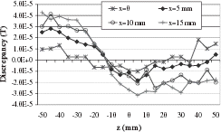
Analysis of Systematic Errors In this experiment, there are random and systematic measurement errors. Systematic errors result from two causes. The first one concerns the zero errors of the measurement equipment. The second one is linked with the positioning of the probe. To illustrate the influence of the probe positioning errors, we plot the discrepancy between the field produced by the theoretical current density and the measured field. The results obtained for different values of x and z are presented in Fig. 11. We observe that the discrepancy does not follow a random law but increases with the distance from the coil center. However, this discrepancy is lower than the accuracy of the gaussmeter. Hence, we can conclude that this experimental scheme will enable us to study the stability and the solution of the inverse problem under analysis.

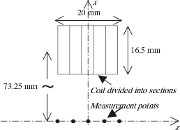
Inverse Problem Under Analysis We assume that the coil is divided into 5 sections. The magnetic field is measured at 5 points equally spaced along a 20-mm long interval on the coil axis (Fig. 12). Their coordinates on the z-axis are thus: −10, −5, 0, 5, and 10 mm. The value of δ² is:

FIGURE 11 Discrepancy between the computed field and the measured field.

FIGURE 12 Experimental inverse problem.

The exact current density is constant and equals to the theoretical current density.

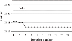
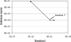
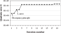
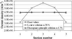
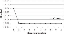
Solution by Iterative Regularization Applying the discrepancy principle, we select the first iteration as the final one (Fig. 13). The use of the L-curve selects iteration 3 (Fig. 14). By plotting the quadratic error versus the number of iterations (Fig. 15), we observe that the discrepancy principle application is efficient to determine the right iteration number. The computed solution (Fig. 16) obtained by this method is in good agreement with the exact solution. The current density is nearly constant in the 5 sections and the maximum relative error between the exact and computed density is only of 1.7%. The use of the L-curve, in this case, produces a less accurate solution. The maximum relative error between the exact and computed density reaches 30%.

FIGURE 13 Application of the discrepancy principle

FIGURE 14 L-curve.

FIGURE 15 Quadratic error versus iteration number.

FIGURE 16 Computed values.

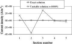
As expected, at the end of the minimization, the computed solution is unstable (Fig. 17). Positive and negative oscillations around the exact values appear.

FIGURE 17 Unstable solution.

These experimental tests show that the proposed method enables us to compute stable solutions for the inverse problem considered.

D-optimal Experimental Design

The purpose of this section is to present the computation of a D-optimal experimental design [8,14] and to illustrate that this plan increases the accuracy of the inverse problem solutions in both numerical and experimental tests.

Theoretical Results We assume additive, independent errors of zero mean and constant variance. With the least squares estimator, the estimation of the parameters J is given by (5) where the matrix M _F = A ^T A is called the information matrix. It has been demonstrated that:

where V is the variance–covariance matrix of the parameters, and σ ² is the standard deviation of the measurement error. So the variance of the estimated parameters depends not only on the variance of the measurement errors but also on the experimental design through the model matrix A. A D-optimal design consists in maximizing the determinant of the information matrix. This ensures that the generalized variances of the parameters are minimized, and that the volume of the confidence region of the estimated parameters is minimal.

Computations We choose to take as many measurement points as unknown currents in order to minimize the number of measurements. In this case, A is a square matrix and:

So we minimize:

To take into account the physical limitations of experiments, we minimize (17) under constraints. We use the projected conjugate gradient algorithm. The gradient in a u direction is calculated by:

The derivative of det(A) is the sum of the determinants obtained by derivation of each row of A. The descent parameter is numerically computed by a golden section algorithm.

Numerical Results We consider the superconducting magnet of Fig. 18 made of 6 coils. The classic choice for the experimental design would be to take the measurements on the surface of the VOI.

FIGURE 18 Magnet shape and experimental designs.

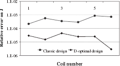
We compute the D-optimal experimental points following the method presented in the preceding section. As the measurements are not possible in the cryostat, we limit the y-coordinate to 0.35 m. The computed positions are presented in Fig. 18. The 4 central points are located on the 0.35-m limit. We observe that the D-optimal points are much nearer to the field sources. The determinant of the information matrix and the condition number of A are given in Table I. The increase in the determinant corresponds with an improvement in the condition number of A. As a result, the inverse problem is more stable. The comparison between the accuracy of the computed current densities for both designs shows a significant improvement (Fig. 19).

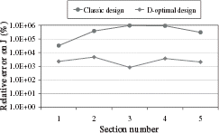
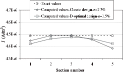
Experimental Results We consider the resistive coil divided into 5 sections and we search for the D-optimal experimental design to reconstruct the 5 current densities. As for MRI magnets, the classic experimental design is composed of 5 measurement points located on a circle where the field is highly homogeneous. In this experiment, the field is about 10-ppm homogeneous on a 2-mm radius circle (Fig. 20). For the computation of the D-optimal points, the z-coordinate is limited to 50 mm and the x-coordinate to 25 mm because of the displacement tables ranges. The computed positions are presented in Fig. 20. We observe, as for the numerical test, that the points are located on the x-limit and that they are nearer to the coil. The determinant of the information matrix and the condition number of A are given in Table II.

TABLE I Determinant and condition number

	Classic design	D-Optimal design
−log(det(M F ))	111	100
Condition number	503	5

FIGURE 19 Accuracy obtained for both designs.

FIGURE 20 Comparison of a classic and D-optimal experimental design.

TABLE II Determinant and condition number

	Classic design	D-optimal design
−log(det(MF))	122	113
Condition number	10^10	10^5

We observe an improvement in the condition number of A. Thus, the solutions obtained by direct inversion of A are better with D-optimal experimental design (Fig. 21). However, the limitation of the probe position prevents the D-optimal design from being stable, so regularization is needed.

FIGURE 21 Relative errors for the direct inversion solutions.

The regularized solutions are presented in Fig. 22. We observe that the D-optimal points produce only a small improvement in the error e. From our point of view, this fact can partly be explained by the increase in the systematic error as the distance to the coil center grows. The improvement in the random errors achieved by the use of the D-optimal design is counterbalanced by the increase in the systematic errors. Moreover, even with the classic design, the solutions are very accurate considering the measurement system. Thus, a large improvement is not possible.

FIGURE 22 Exact and regularized solutions for D-optimal and classic designs.

The conclusion is that the construction of a D-optimal experiment for an inverse problem improves the stability of the problem and the accuracy of solutions when the experimental conditions are favorable.

Nonlinear Inverse Problem

Inverse Problem Statement

The problem is to reconstruct the dimensions of the coils and particularly the coils axial positions from measured magnetic field values. The integral equation to be solved is again (2). However, we observe that the kernel of this equation depends on the coil position z _M . Thus, the inverse problem is nonlinear. We assume that the current density, coil geometry, and coil radius are known, the unknowns are the coils axial positions denoted as Z. The discretization of (2) leads to a formulation of the type:

where A depends on the coil positions Z.

Solution of the Nonlinear Inverse Problem

Computations The computations of the coil geometric dimensions Z are performed with the same principles as in the linear case. The objective function is expressed as:

In the minimization procedure, the gradient is computed as:

The derivative of A with respect to the coil axial positions is computed by derivation of (2) with respect to the integral bounds in z. The descent direction is computed by (8). The descent parameter is chosen as the linear estimation of the solution of the one variable minimization.

This enables us to avoid the use of a numerical line search.

Choice of the Regularization Parameter The method used is the discrepancy principle. Iterations are stopped when:

Uniqueness of the Solution In general, different arrangements of coils may produce the same magnetic field at the measurement points and the minimization procedure may lead to another solution than the actual one. In the example that we tested, we observed that for moderate inverse problems i.e. few unknowns only, with a starting point for the minimization not too far from the actual solution, the minimization tends to the actual solution. In other cases, the problem of the non uniqueness appears. However, our problem is usually a moderate one: the starting points for the minimization are the coil specifications and the displacement that we try to identify is a small one, even if its influence on the field is high. Therefore, in those cases, we were able to overcome this difficulty.

Numerical Example

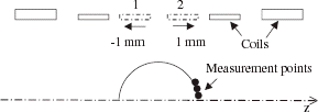
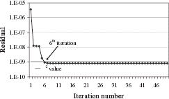
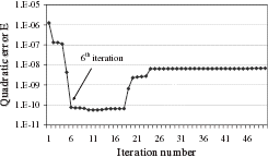
The problem under consideration is the diagnosis of a magnet that presents a low homogeneity due to a manufacturing error. Some of its coils have an incorrect axial position. As a test case, we use the magnet represented schematically in Fig. 23. A defect is simulated by a 1-mm displacement of the central coils. We simulate experimental measurements by adding a uniformly distributed random noise of 10 ppm to the exact field values. We use 29 measurement points on the VOI surface. The starting points of the minimization are the coil theoretical values, i.e. the positions prescribed by the manufacturing process. All coils are allowed to move. Selecting the final iteration using exact δ ² leads to stopping the minimization at the 6th iteration (Fig. 24). For this iteration, we observe that the quadratic error E is minimal (Fig. 25).

FIGURE 23 Geometry of the nonlinear numerical example.

FIGURE 24 Application of the discrepancy principle.

FIGURE 25 Quadratic error versus iteration number.

By comparing the exact values and the regularized solution (Table III), we observe that we are able to compute the simulated defects.

TABLE III Computed defects for the regularized solution

	Exact displacement (mm)	Computed displacement (mm)	Relative error (%)
Coil 1	−1	−0.994	0.6
Coil 2	1	0.992	0.8

At the end of the minimization, the accuracy of the computed solution is lower, but no large oscillations in the computed values are observed (Table IV). This fact can be explained by the physical nature of the inverse problem to be solved. Large instability in the solution occurs when the unknown values increase in magnitude and take different signs to produce exactly the measured field. In this problem, a large increase in the coil axial positions while all other parameters remain constant would produce a much lower magnetic field than the measured one. Thus, the instability is limited.

TABLE IV Computed defects for the unstable solution

	Exact displacement (mm)	Computed displacement (mm)	Relative error (%)
Coil 1	−1	−0.892	10.8
Coil 2	1	1.10	10

Experimental Validation

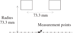
We use two Helmholtz air coils (Fig. 26) with the same experimental scheme presented in Fig. 10. These coils, which are separated by a distance equal to their radius, produce a homogeneous field at the center of the system [9]. The magnetic field is measured in 2 points on the coil axis. Their coordinates on the x-axis are −2.5 and 2.5 mm. We compute the coil axial positions from these two field measurement. We apply the iterative regularization with the discrepancy principle (Fig. 27). We observe that the computed positions match the exact values (Table V).

FIGURE 26 Helmholtz coils under analysis.

FIGURE 27 Application of the discrepancy principle.

TABLE V Exact and computed positions

	Exact position (mm)	Computed position (mm)	Relative error (%)
Coil 1	−36.65	−36.77	0.3
Coil 2	36.65	36.77	0.3

So, the numerical and experimental tests illustrate the efficiency of the proposed method to reconstruct the coil axial positions.

Conclusion

The authors have presented iterative regularization applied to a linear and nonlinear inverse problem of magnetostatics. The numerical and experimental tests show that in a magnet it is possible to find the current density or a faulty coil axial position with measured field values as input data. The method used always produces better results than the usual least squares solution. For unstable problems, this improvement is significant, as the regularized solutions are close to the exact ones, while the least square solutions are strongly distorted. The authors have computed D-optimal experimental designs to reconstruct the current densities and show that this approach improves the stability of inverse problems and the accuracy of their solutions.

Nomenclature

Table

A	=	matrix of the contribution of each coil to each field value
B	=	magnetic field values (T)
e	=	maximum relative error on the estimated parameters (%)
E	=	quadratic error between the exact and computed solution
J	=	coil current densities (A/m^2)
M F	=	information matrix
MRI	=	magnetic Resonance Imaging
R	=	quadratic residual between the computed and measured field
VOI	=	volume Of Interest
Z	=	coil axial positions (m)
δ^2	=	level of experimental error

Additional information

Notes on contributors

J.M. Kauffmann

*This article was presented at the 4th International Conference on Inverse Problem in Engineering, Rio de Janeiro, Brazil, 2002.

Notes

*This article was presented at the 4th International Conference on Inverse Problem in Engineering, Rio de Janeiro, Brazil, 2002.

References

- Romanov VG Kabanikhin SI 1994 Inverse Problems for Maxwell's Equations, VSP
- Nenonen JT 1994 Sept. Solving the inverse problem in magnetocardiography IEEE Engineering in Medicine and Biology 487
- Bettini P et al. 2001 Identification of the plasma magnetic contour from external magnetic measurements by means of equivalent currents Eur. Phys. J. AP 13 51
- Russenschuck S et al 1998 Integrated design of superconducting accelerator magnets. A case study of the main quadrupole Eur. Phys. J. AP 1 93
- Alifanov OM Artyukhin EA Rumyantsev SV 1995 Extreme Methods for Solving Ill-posed Problems with Applications to Inverse Heat Transfer Problems., Begell house
- Gilyazov SF Gol’dman NL 2000 Regularization of Ill-posed Problems by Iteration Methods, Kluwer academic publishers
- Bégot , S , Voisin , E , Hiebel , P , Kauffmann , JM and Artioukhine , E . 2002 . Resolution of linear and a nonlinear inverse problem in magnetostatics . Eur. Phys. J. AP , 19 ( 2 ) : 141
- Bégot , S , Voisin , E , Hiebel , P , Kauffmann , JM and Artioukhine , E . 2002 . D-optimal experimental design applied to a linear magnetostatic inverse problem . IEEE Trans. Magn, , 38 ( 2 ) : 1065
- Jackson JD 1999 Classical Electrodynamics 3rd Edn. Wiley New York
- Tikhonov AN Arsenin V 1974 Methods for Solving Ill-posed Problems Mir
- Gill PE Murray W Wright MH 1981 Practical optimization, Academic Press New York
- Hansen PC 1993 The use of the L-curve in the regularization of discrete ill-posed problems SIAM J. Sci. Comput 14 6 1487
- Barlow R 1989 Statistics, Wiley
- Fedorov VV 1972 Theory of Optimal Experiments, Academic Press