Identification of velocity distribution in a turbulent flow inside parallel-plate ducts from wall temperature measurements

Abstract

An Inverse Heat Convection Problem is investigated in this numerical study. Turbulent forced convection is considered, with a hydrodynamically fully developed, thermally developing, incompressible, constant property flow inside a parallel-plate duct. Velocity and effective diffusivity distributions of the turbulent model are characterised by a Reynolds number b ⁺ based on the shear stress velocity.

The identification of b ⁺ from simulated wall temperature measurements is presented. A heat flux density is applied along the channel length and temperature responses are taken at the wall external surface. Heat transfer has to act as a small but measurable perturbation of the flow.

The inverse problem is recast into an optimisation problem solved with a Quasi-Newton method. Reynolds numbers 10⁵ and 10⁶, corresponding to two different values of b ⁺ , are considered. Effects of sensor number and location, as well as magnitude of measurement error on the estimation accuracy, are examined.

Introduction

Forced convection in turbulent flow inside ducts is frequently encountered in industrial equipment. Many available studies are concerned with the direct problem, that is: having a mathematical model and knowing boundary conditions, one searches to compute the temperature field over the whole domain. Applications in which thermophysical properties, geometric characteristics or boundary conditions are unknown, but temperature measurements are locally available, belong to the inverse problems research area i.e. from the knowledge of experimental data, one searches to estimate the unknowns.

The field of Inverse Heat Conduction Problems has already been intensively covered but inverse problems related to convective heat transfer have been studied much less. One of the earliest complete studies is due to Moutsoglou [1]. He was interested in an inverse free convection problem for the estimation of wall spatial temperature and heat flux density distributions in a parallel-plate duct, using a function specification method [2]. Other works deal with inverse natural convection in cavities, for the estimation of wall heat flux densities [3–6] and also internal heat sources using a low order model [7,8].

Inverse forced convection problems have received more attention, certainly because they are simpler. Most of the available works are concerned with linear inverse problems. Several studies deal with laminar flows in parallel-plate ducts and cover different kinds of estimation: spatial distribution of wall heat flux density [9], timewise variation of inlet temperature [10], inlet temperature profile [11], wall heat flux density varying with space and time [12], time-dependant wall heat flux density for a non-Newtonian fluid flow [13]. In all these studies the iterative regularisation method [14] (conjugate gradient method coupled with the resolution of the direct, sensitivity and adjoint problem, and use of the discrepancy principle) is used. The simplex method has also been used to estimate spatial distribution of wall heat flux density [15]. A non-iterative method based on the state space representation has been used to estimate both inlet temperature and wall heat flux density for a circular duct with steady-state laminar flow [16], along with A 3D problem for the estimation of time-varying wall heat flux density using the iterative regularisation method [17].

Turbulent regime has been investigated in a few studies involving the identification of boundary conditions. Estimation of timewise variation of wall heat flux applied to a parallel-plate duct has been performed by Liu and Özisik [18] using the conjugate gradient method with an adjoint problem. A non-iterative sequential method using a low order model has been proposed by Girault et al. [19] to simultaneously estimate timewise variation of two wall heat fluxes applied to a parallel-plate duct. For the thermal steady state, estimation of spatially non uniform wall heat flux in circular pipe flow has been made by Su et al. [20] using the Levenberg–Marquardt algorithm.

Non-linear inverse forced convection problems are not numerous. Among them can be noticed the estimation of the inlet temperature profile in a circular duct flow of a non-Newtonian fluid with temperature-dependant properties [21], and the identification of wall heat flux density varying along a parallel-plate duct flow in steady-state, the thermal conductivity of the fluid being temperature-dependant [22].

All above studies are concerned with the estimation of boundary conditions. In the present work another class of inverse problems is investigated. A turbulent flow inside a parallel-plate duct is considered and the possibility to use heat transfer as a small perturbation of the flow to estimate a parameter characterising velocity and effective diffusivity distributions is explored in this numerical study. A known heat flux density is applied on the upper and lower plates of the duct. Temperature responses, that depend on the unknown, are taken at the wall external surface. A squared residues functional built with these data and the heat transfer model solution has then to be minimised to estimate the unknown. The basic idea of using temperature or concentration measurements to get information about velocity field has been under development for the last decades. Mass transfer is often used for a detailed study of the near wall region. As examples, turbulent fluctuations in the velocity gradient at the wall have been estimated by Mao and Hanratty [23,24] using the measure of a mass transfer coefficient. The fluid is kept isothermal and mass transfer does not induce perturbations in the flow. Heat transfer is less frequently used. For instance, a thermal flow meter based on the correlation between solid–fluid exchange coefficient and mass flow rate, but without an inverse problem formulation, has been built and tested [25].

In this paper, the system is first described, governing heat transfer equation and associated boundary conditions are written and the turbulent model is presented. The inverse problem is then formulated. Configurations under consideration are detailed and sensors sensitivities are studied. Finally, results for several inversion cases are presented and discussed.

System Description

Physical Problem

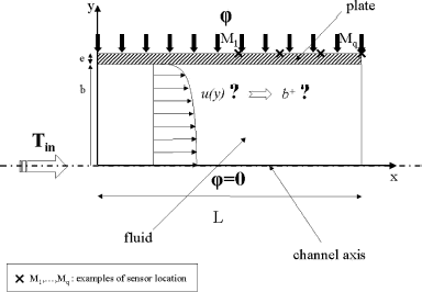
Let us consider turbulent forced convection, with a hydrodynamically fully developed, thermally developing, incompressible, constant property, turbulent flow inside a parallel-plate smooth duct. Axial conduction in the fluid and viscous dissipation are neglected. Conduction along the flow in the wall material is disregarded. The assumption of uniform wall temperature across the whole thickness of the plates is made. Both plates are subjected to the same heat flux density. The channel axis being then a symmetry axis, only half of the duct is considered. A schematic view of the system is presented hereafter in Fig. 1.

FIGURE 1 System description.

Governing Equations

For such a problem, the characteristic heat flux density is the applied heat flux density ϕ. A characteristic temperature difference can then be defined as:

So, by choosing a dimensionless applied heat flux as:

and introducing the following dimensionless quantities:

the dimensionless governing steady state energy equation is written as [26]:

with following boundary conditions, considering the channel axis symmetry:

where is the dimensionless length of the channel.

The direct problem consists in the resolution of Eq. (2a). A numerical solution approximation is obtained with the Finite Volume Method. Equation (2a) being linear and parabolic in ξ, the solution is obtained by using a spatially marching procedure in the ξ direction. An appropriate typical mesh uses 21 nodes in the ξ direction (regular mesh) and 30 in the η direction (non-regular mesh, refined near wall).

Turbulent Model

The dimensionless fully developed turbulent velocity distribution U(η) and the dimensionless effective diffusivity ε_eff(η) in Eq. (2a) are determined by a pseudo-laminar turbulent model given by Kim and Özisik [27] and presented below, except for the turbulent Prandtl number: , which has been taken by Jischa and Rieke [28] as:

In a classical way, the turbulent model is expressed with new dimensionless variables.

is called the shear velocity, where is the wall shear stress depending on the gradient of pressure dP _m /dx which has generated the flow, and the fluid density ρ. A Reynolds number based on the shear stress velocity may be written as:

Defining a new dimensionless transverse coordinate y ⁺ = (1−η)b ⁺, b ⁺ may also be seen as the dimensionless transverse coordinate at the channel axis (η = 0). A new dimensionless velocity u ⁺ = u/u _τ is introduced.

The turbulent velocity distribution is taken as the following three-layer model [27]:

1.	Viscous sub-layer:
2.	Buffer layer:
3.	Turbulent core: The turbulent viscosity distribution is taken as the two-layer model [27]: for y+<40, with k 1 = 0.407 and E = 10 with k 2 = 0.4

Turbulent velocity and viscosity distributions are therefore characterised by the parameter b ⁺ .

The Reynolds number is given by:

U(η) and ε_eff(η) are given by:

And

Inverse Problem

Formulation

Suppose that b ⁺ is unknown and inlet temperature is known. In order to identify b ⁺ , a known heat flux density is applied on both upper and lower plates along the channel length and temperature responses are taken at the wall external surface. These measurements are dependent on the way that heat is transported in the flow. Thus they depend on b ⁺ . The inverse procedure consists in the determination of b ⁺ from these simulated temperature data.

Note the Reynolds number Re based on mean velocity could have been chosen as the dimensionless parameter to be identified in the inverse procedure, but the choice of b ⁺ has been made for the following two reasons:

1.	As (c.f. Eq. (4)), the gradient of pressure which has generated the flow appears formally in the expression of b + , allowing a direct access to this quantity (or the corresponding wall shear stress τw).
2.	If Re is the unknown parameter, then for each iteration of the inverse algorithm, Re has its current value and b + needs to be calculated to obtain u + . This involves, for each iteration, the resolution of Eq. (6) which is transcendental in that case. A larger computing time for inversion is then needed.

The inverse problem consisting in the identification of b ⁺ may be formulated as an optimisation problem: find b ⁺ minimising the squared residues functional f(b ⁺ ) defined as:

where the are the Nmes dimensionless temperature measurements taken at the wall external surface.

According to previous assumptions about the wall material, the are obtained from the dimensionless temperatures at the fluid–solid interface coming from the resolution of Eq. (2), by a simple heat flux balance:

where λ* = λ _s  b/λ _f  e.

Magnitude of Applied Heat Flux Density

The applied heat flux density ϕ has to be chosen as a satisfying compromise between two opposite considerations: a high ϕ to obtain high sensitivities of the sensors with respect to b ⁺ , and a low ϕ to induce the slightest possible perturbation of the flow. In fact, when heating the channel, the flow may be modified by two ways: generation of natural convection and variation of the fluid properties. To prevent such events, the mean increase of temperature induced by ϕ should not be greater than a few Kelvin. This will be verified a posteriori.

Optimisation Algorithm

A Quasi-Newton method [29] is used to minimise f (b ⁺ ) defined by Eq. (9). This method is briefly presented in the following paragraphs.

The basic Newton method consists of an approximation of the objective function f around the current iterate by a quadratic function, that is a second order Taylor's expansion. The next iterate will be where the search direction s _k is the minimiser of the quadratic function and is obtained by writing the first order condition, leading to:

The second order condition requires the positiveness of , which is not always assured, depending on the initial guess. The convergence is guaranteed only if the starting point is sufficiently close to a local minimiser b ⁺ * at which f„ is positive. A Quasi-Newton method is used to ensure the convergence when the initial guess is not close to a minimiser. It uses a line-search method: the next iterate is obtained by where β _k is chosen so that and to satisfy the curvature condition, and the search direction s _k is not obtained by Eq. (11) but by:

where H _k is an updated approximation to .

The gradient is given by:

Its calculation requires the computation of the sensitivities . These are approximated with Forward Finite Differences, yielding, for , to:

where γ is a small perturbation factor.

The numerical evaluation of the gradient then requires a second resolution of the direct problem (Eq. (2)) in addition to the one needed to compute . The computation of would then require to solve three direct problems. To avoid such a time-consuming operation, is approximated by H _k , using quantities and . Formulas for H _k and β _k can be found in [29].

The general algorithm may be summarised as:

1.	Using the current iterate bk +, compute u + with Eq. (5a,b,c) and with Eq. (5d,e)
2.	Compute Re with Eq. (6), U with Eq. (7) and εeff with Eqs. (8) and (3).
3.	Solve Eqs. (2a,b,c,d) to obtain . Compute using Eq. (10) and with Eq. (9).
4.	Repeat Steps 1 to 3 with (γ small) and compute sensitivities using Eq. (14).
5.	Compute using Eq. (13).
6.	Compute H k , then s k with Eq. (12) and β k .
7.	Set the next iterate to: .
8.	Go to Step 1 and set k = k+1.

This iterative procedure is performed until the chosen stopping criterion (c.f. Eq. (15), Eq. (17) and following remark) is satisfied.

For a rectangular duct section, the laminar-turbulent transition corresponds to Re ≅ 2400 (i.e. b ⁺ ≅ 50). Therefore it seems logical to take 50 as lower bound for b ⁺ . This value will also be taken as initial guess for the minimisation algorithm, according to sensitivity analysis.

The Studied Configurations

The following case is considered: water at T _in = 300K is entering through the region of the channel subjected to the applied heat flux density. Fluid properties are then taken as:

1.	ν = 8.58 × 10−7 m2 s−1
2.	α = 1.47 × 10−7 m2 s−1
3.	λf = 0.61 W m−1 K−1

The solid thermal conductivity is taken as λ_s = 14.9 W m⁻¹ K⁻¹. The half channel height is b = 5 × 10⁻² m and the domain length used to heat the wall channel and to simulate the temperature experimental data is L = De = 4b = 0.2 m where De = 4b is the equivalent diameter. The wall thickness is e = 2 × 10⁻³ m. Two values of b ⁺ are considered: b ⁺ = 1166 and b ⁺ = 9361, corresponding respectively to Re ≅ 10⁵ and 10⁶. Corresponding test cases are called respectively Cases 1 and 2.

The applied heat flux density ϕ is chosen to be:

1.	ϕ = 1750 W m−2 for the case b + = 1166
2.	ϕ = 13000 W m−2 for the case b + = 9361

According to Eq. (1), values of ▵T _ref are then 142.74 and 1060.36 K for Cases 1 and 2 respectively.

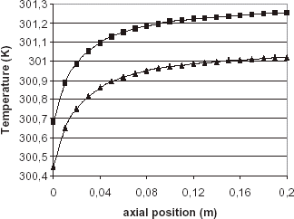
Figure 2 shows temperatures at solid–fluid interface and wall external surface (21 positions in the axial direction) for Case 1.

FIGURE 2 (▴) and (▪) with respect to axial position, for case 1.

It can be verified that temperature at solid–fluid interface and x = L, which is the hottest point in the fluid domain, is about 301 K, corresponding to an increase of only 1K from T _in. The assumption of an unchanged flow is then expected to be valid. It is also verified for Case 2.

Sensitivity Analysis

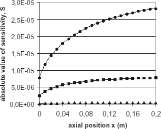
The applied heat flux density ϕ = 1750 W m⁻² is considered. Temperatures are not linear functions of b ⁺ , consequently sensitivities are dependent on b ⁺ . Let us call S the absolute value of the sensitivity given by Eq. (14):

Figure 3 shows the values of S at possible sensors locations for three values of b ⁺ (500, 1000 and 5000). Results were intuitively expected. It is verified that for a given b ⁺ , S increases with the axial location x along the heated channel. If only one sensor is used, the best possible location is then at x = L. For a given location, the larger b ⁺ , the lower S is. Hence, it seems useful to start with b ⁺ = 50 as initial guess to ensure the highest possible sensitivities during first iterations.

FIGURE 3 Values of S for the 21 nodes, for b ⁺ = 500 (•), 1000 (▪) and 5000 (▴).

Inversion Results and Analysis

Validation with

Inversion using “exact” temperatures gives excellent results whatever the number and position of sensors. Results obtained with a single sensor located in x = L (node 21) are given for Cases 1 and 2 (c.f. Table I). One should note that the stopping criterion for the minimisation algorithm is:

TABLE I Identification results for different test cases. Estimated values of b ⁺ and relative errors

	CASE 1 Exact value b ^+ = 1166 ( Re ≅ 10^5 )	CASE 2 Exact value b ^+ = 9361 ( Re ≅ 10^6 )
Node 21 σ = 0 K	1166.107 (0.009 %)	9361.001 (0.000014%)
Node 21 σ = 3.88 × 10^−2 K	1097.682 (5.859 %)	8889.011 (5.042 %)
4 Nodes (18–21) σ = 3.88 × 10^−2 K	1098.981 (5.748 %)	8989.315 (3.971%)
4 Nodes (6,11,16,21) σ = 3.88 × 10^−2 K	1103.986 (5.318 %)	9011.175 (3.737%)
6 Nodes (16–21) σ = 3.88 × 10^−2 K	1145.635 (1.747 %)	9172.593 (2.013%)
6 Nodes (6,9,12,15,18,21) σ = 3.88 × 10^−2 K	1146.509 (1.672 %)	9190.534 (1.821%)
16 Nodes (6–21) σ = 3.88 × 10^−2 K	1169.558 (0.305 %)	9378.425 (0.186 %)
16 Nodes (6–21) σ = 10^−1 K	1174.952 (0.768 %)	9406.627 (0.487 %)

Simulation of Real Measurements

Simulated temperatures are generated by adding random errors to temperatures computed with Eqs. (2) and Eq. (10) for applied heat flux density ϕ. That is:

where σ is the dimensional standard deviation of measurement errors which is assumed to be the same for all measurements, ω is a normally distributed random number, meaning there is a 99% probability of the value of ω lying in the range −2.576<ω<+ 2.576 and ▵T is the measurement error. Thus:

−10⁻¹ K<▵ T < + 10⁻¹ K corresponds to σ = 3.88 10⁻² K

and

−2.576 × 10⁻¹ K<▵T < + 2.576 × 10⁻¹ K corresponds to σ = 10⁻¹ K.

When a single sensor is used, ▵T = + σ is taken.

The discrepancy principle [14] is used to obtain the following stopping criterion:

If this criterion is not satisfied in the iterative process, the algorithm is stopped after a chosen number of iterations without decreasing f (b ⁺ ).

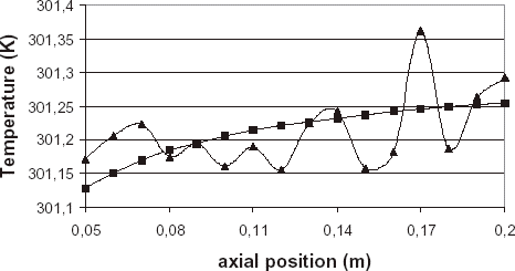
Considering the analysis of sensitivities to b ⁺ and the mesh sensitivity, Nodes 1 to 5 have not been taken as sensors. In Fig. 4 are shown both simulated exact and “measured” dimensional temperatures for Case 1 with σ = 3.88 × 10⁻² K.

FIGURE 4 (▪) and (▴) at nodes 6–21 (case 1 with σ = 3.88 × 10⁻² K).

Effect of Sensor Number and Measurement Errors

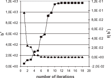
Let us consider a single sensor measurement. The Node 21 is chosen and a simulated error ▵T = + σ = 3.88 × 10⁻² K is added. One can note (see Table I) that the solution b ⁺ is underestimated (relative error ≈ 5 to 6%) for both Cases 1 and 2. More sensors need to be used in the presence of measurement error. The inverse problem is then overdetermined since it has more data than unknowns. Table I shows results for Case 1 and σ = 3.88 × 10⁻² K when 4, 6 and 16 sensors are used. With 4 sensors, the results quality is not clearly improved, but with 6 sensors, results become more satisfying, and with 16 sensors the estimation is accurate. For this last case, Fig. 5 shows the convergence of f(b ⁺ ) and b ⁺ with respect to iteration number.

FIGURE 5 Convergence of f(b ⁺ ) (▴) and b ⁺ (▪) with respect to iteration number (case 1, sensors at nodes 6–21, σ = 3.88 × 10⁻² K).

When noise level is increased to σ = 10⁻¹ K, the estimation using Nodes 6 to 21 as sensors is slightly deteriorated but remains very good (relative error with the exact value <1%).

Case 2 is now considered. As b ⁺ is increased in comparison with Case 1, sensitivities should be lower but this is compensated by a higher value for the applied heat flux ϕ. Moreover, wall external temperature data are higher and therefore less sensitive to additive noise. As a consequence, estimations are as good as those of Case 1 (c.f. Table I).

Effect of Sensor Location

As it can be seen in Table I, for Case 1 and a given number of sensors (4 or 6), the estimation with sensors close to x = L is worse than the one obtained with sensors equally positioned between Nodes 6 and 21. This seems strange because the closer the sensors are to L, the higher are their sensitivities. Nevertheless, this may be explained by the fact that data close to L present redundant information, especially in presence of noise.

Reconstruction of Turbulent Quantities

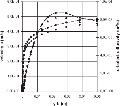
Once b ⁺ has been identified, estimated profiles of velocity u and turbulent diffusivity α_turb are obtained using Eqs. (5a–e), (6), (7), (8) and (3). Figure 6 shows reconstructed profiles for Case 1 and two configurations of inversion: a single sensor (Node 21) and 16 sensors (Nodes 6 to 21), with σ = 3.88 × 10⁻² K.

FIGURE 6 Reconstructed velocity and turbulent diffusivity profiles for case 1 with σ = 3.88 × 10⁻² K. “Exact” values: u (—), α_turb (-·-·-·). Estimations with node 21: u (♦), α_turb (▴). Estimations with nodes 6–21: u (•), α_turb (▪).

Conclusions

An inverse problem of turbulent forced convection inside a parallel-plate duct has been investigated in this numerical study. In order to estimate a Reynolds number b ⁺ based on the shear stress velocity and characterising turbulent velocity and effective diffusivity distributions, a known heat flux density is applied on the upper and lower plates of the duct, and temperature responses dependent on b ⁺ are taken at the wall external surface. A squared residues functional built on these data and a heat transfer model has been minimised to estimate the unknown.

A total of 16 different configurations for inversion have been presented, including the estimation of 2 values of b ⁺ corresponding to Re ≅ 10⁵ and 10⁶, using exact data and simulated data with 2 noise levels, and an analysis of the influence of sensors number and position. Results have shown that such a procedure allows us to accurately estimate b ⁺ even if the measurements are altered with errors, provided that the number of sensors may be sufficiently large.

Cases of velocity and diffusivity laws involving more unknown parameters can be handled with the presented methodology. Appropriate sensors with adapted sensitivities are then necessary.

The method described in this article may be used in conjunction with a heating device and temperature sensors to obtain a thermal flow meter for established turbulent flows in ducts.

Nomenclature

Table

b	=	channel half-height (m)
b ^+	=	Reynolds number based on shear stress velocity =
De	=	equivalent diameter (m)
e	=	wall thickness (m)
f	=	squared residues functional to minimise
f’, f„	=	first and second derivatives of f with respect to b ^+
H	=	approximation to f”
L	=	channel length, m
L*	=	dimensionless channel length
Nmes	=	number of measurements
Pe	=	Péclet number
P m	=	motion pressure, Pa
Pr	=	Prandtl number
Prturb	=	turbulent Prandtl number
Re	=	Reynolds number based on mean velocity
S	=	absolute value of sensitivity
s	=	search direction of the minimisation algorithm
T	=	temperature (K)
U	=	dimensionless velocity = u/u m
u τ	=	shear stress velocity (m s^−1)
u	=	velocity (m s^−1)
u m	=	fluid bulk mean velocity = (m s^−1)
u ^+	=	dimensionless velocity = u/u τ
x	=	axial coordinate (m)
y	=	transverse coordinate (m)
y ^+	=	dimensionless transverse coordinate = (1−η)b ^+

Greek Symbols

Table

α	=	fluid thermal diffusivity (m^2 s^−1)
αturb	=	turbulent diffusivity for heat (m^2 s^−1)
▵T	=	measurement error (K)
▵T ref	=	characteristic temperature difference (K)
εeff	=	dimensionless effective diffusivity for heat
Φ	=	dimensionless applied heat flux = 1
η	=	dimensionless transverse coordinate = y/b
ϕ	=	applied heat flux density (W m^−2)
λ	=	thermal conductivity (W m^−1 K^−1)
λ*	=	solid–fluid thermal conductance ratio
ν	=	fluid kinematic viscosity (m^2 s^−1)
νturb	=	turbulent viscosity (m^2 s^−1)
θ	=	dimensionless temperature
ρ	=	fluid density (kg m^−3)
σ	=	standard deviation of added noise (K)
τ	=	shear stress (Pa)
ω	=	random number
ξ	=	dimensionless axial coordinate

Subscripts not Previously Introduced

Table

f	=	relative to fluid
in	=	inlet
k	=	index for current iteration of the minimisation algorithm
s	=	relative to solid
surf	=	at wall external surface
w	=	at wall i.e. at solid–fluid interface

Superscripts not Previously Introduced

Table

calc	=	calculated
mes	=	measured

References

- Moutsoglou , A . 1989 . An inverse convection problem . Journal of Heat Transfer , 111 : 37 – 43 .
- Beck JV Blackwell B St Clair CR 1985 Inverse Heat Conduction: Ill-posed Problems, John Wiley & Sons New York
- Prud’homme , M and Nguyen , TH . 1997 . Whole time-domain approach to the inverse natural convection problem . Numerical Heat Transfer, Part A , 32 : 169 – 186 .
- Park , HM and Chung , OY . 1999 . Inverse natural convection problem of estimating wall heat flux using a moving sensor . Journal of Heat Transfer , 121 : 828 – 836 .
- Park , HM and Chung , OY . 2000 . Inverse natural convection problem of estimating wall heat flux . Chemical Engineering Science , 55 : 2131 – 2141 .
- Prud'homme , M and Nguyen , TH . 2001 . Solution of inverse free convection problems by conjugate gradient method: effects of Rayleigh number . International Journal of Heat and Mass Transfer , 44 : 2011 – 2027 .
- Park , HM and Jung , WS . 2001 . The Karhunen-Loève Galerkin method for the inverse natural convection problems . International Journal of Heat and Mass Transfer , 44 : 155 – 167 .
- Park , HM and Chung , JS . 2002 . A sequential method of solving inverse natural convection problems . Inverse Problems , 18 : 529 – 546 .
- Huang , CH and Özisik , MN . 1992 . Inverse problem of determining unknown wall heat flux in laminar flow through a parallel plate duct . Numerical Heat Transfer, Part A , 21 : 55 – 70 .
- Bokar , JC and Özisik , MN . 1995 . An inverse analysis for estimating the time-varying inlet temperature in laminar flow inside a parallel plate duct . International Journal of Heat and Mass Transfer , 38 ( 1 ) : 39 – 45 .
- Liu , FB and Özisik , MN . 1996 . Estimation of inlet temperature profile in laminar duct flow . Inverse Problems in Engineering , 3 : 131 – 143 .
- Machado , HA and Orlande , HRB . 1997 . Inverse analysis for estimating the timewise and spacewise variation of the wall heat flux in a parallel plate channel . International Journal for Numerical Methods for Heat and Fluid Flow , 7 ( 7 ) : 696 – 710 .
- Machado , HA and Orlande , HRB . 1998 . Inverse problem for estimating the heat flux to a non-Newtonian fluid in a parallel plate channel . Journal of the Brazilian Society of Mechanical Sciences , 20 ( 1 ) : 51 – 61 .
- Alifanov OM 1994 Inverse Heat Transfer Problems, Springer-Verlag New York
- Ben Abdallah , P , Sadat , H and Le Dez , V . 2000 . Résolution d'un problème inverse de convection-diffusion par une méthode de perturbation singulière . International Journal of Thermal Sciences , 39 : 742 – 752 .
- Hsu , PT , Chen , CK and Yang , YT . 1998 . A 2-D inverse method for simultaneous estimation of the inlet temperature and wall heat flux in a laminar circular duct flow . Numerical Heat Transfer, Part A , 34 : 731 – 745 .
- Huang , CH and Chen , WC . 2000 . A three-dimensional inverse forced convection problem in estimating surface heat flux by conjugate gradient method . International Journal of Heat and Mass Transfer , 43 : 3171 – 3181 .
- Liu , FB and Özisik , MN . 1996 . Inverse analysis of transient turbulent forced convection inside parallel-plate ducts . International Journal of Heat and Mass Transfer , 39 ( 12 ) : 2615 – 2618 .
- Girault M Petit D Videcoq E 2002 Inverse problem of turbulent forced convection inside parallel-plate ducts using a reduced model 12th International Heat Transfer Conference August 18–23 Grenoble France
- Su , J , Lopes , AB and Silva Neto , AJ . 2000 . Estimation of unknown wall heat flux in turbulent circular pipe flow . International Communications in Heat and Mass Transfer , 27 ( 7 ) : 945 – 954 .
- Gejadze I. I Jarny Y 2001 A method of temperature restoration in polymer melt flow through narrow channel Proc. Eurotherm Seminar No. 68: Inverse Problems and Experimantal Design in Thermal and Mechanical Engineering March 5–7 pp. 247–254 Poitiers France
- Park , HM and Lee , JH . 1998 . A method of solving inverse convection problems by means of mode reduction . Chemical Engineering Science , 53 ( 9 ) : 1731 – 1744 .
- Mao , Z and Hanratty , TJ . 1991 . Analysis of wall shear stress probes in large amplitude unsteady flows . International Journal of Heat and Mass Transfer , 34 ( 1 ) : 281 – 290 .
- Mao , Z and Hanratty , TJ . 1991 . Application of an inverse mass transfer method to the measurement of turbulent fluctuations in the velocity gradient at the wall . Experiments in Fluids , 11 : 65 – 73 .
- Fulcheri , L and Pacher , F . 1992 . Débitmètre thermique non intrusif . Revue Générale de Thermique , 31 ( 365 ) : 311 – 320 .
- Kays WM Crawford ME 1993 Convective Heat and Mass Transfer 3rd Edn. McGraw-Hill Singapore
- Kim WS Özisik MN 1989 Turbulent forced convection inside a parallel-plate channel with periodic variation of inlet temperature Journal of Heat Transfer 111 882 888 Trans ASME
- Jischa , M and Rieke , HB . 1979 . About the prediction of turbulent Prandtl and Schmidt numbers from modeled transport equations . International Journal of Heat and Mass Transfer , 22 : 1547 – 1555 .
- Gill PE Murray W Wright MH 1981 Practical Optimization, Academic Press New York