Backward specification of prior in bayesian inference as an inverse problem

Abstract

Specification of prior distribution is one of the most important methodological as well practical problems in Bayesian inference. Although a number of approaches have been proposed, none of them is completely satisfactory from both theoretical and practical points of view. We propose a new method to infer prior distribution from a priori information which may be available from observations. The method consists of specifying a predictive distribution of the value of interest and then working backwards towards the prior distribution on the parameters. The method requires the solution of the Fredholm integral equation of the first kind, which can be effectively approximated using Tikhonov regularization. Numerical examples for two cases of Bayesian inference are presented.

Keywords:

• Bayesian inference
• Regularization
• Prior distribution
• Likelihood

1. Introduction

Transferring prior beliefs into an exact mathematical form has been, and remains, one of the most controversial and challenging issues of Bayesian inference. The problem is twofold. The first one is how to specify our knowledge in the most succinct and tractable form and the second one is how to transfer prior knowledge of observable variables onto prior knowledge of parameters which are generally unobservable. A number of approaches have been developed, with the most notable ones being: conjugate priors, Jeffreys noninformative priors and empirical Bayesian methods [1,3]. Conjugate priors, although being widely used, can only be justified if enough information is available to believe that the true prior distribution belongs to the specified family; otherwise, the main justification for using conjugate prior is their mathematical tractability. Jeffreys noninformative prior uses the Fisher information matrix to place a maximally noninformative prior on the parameters, exploiting the fact that the Fisher information matrix is widely considered to be an indicator of the accuracy of a parameter estimate. However, this approach can only be effectively used in one-dimensional cases and does not satisfy the likelihood principle [1]. Other problem with noninformative priors is that there might be a number of them for a given problem and there is no clear cut rule which noninformative prior has to be preferred. Empirical Bayesian methods use the marginal distribution of the value of interest to elicit prior distribution on the parameters. The empirical estimation of the prior is strictly speaking a violation of Bayes theorem because the same data set is used for both: estimation of the likelihood and inferring the prior distribution. This approach effectively invalidates Bayes theorem due to the fact that:

The formula (1) means that once the prior probability is conditioned on the current data set, the Bayes formula is no longer valid and we can not formally go ahead with Bayesian inference. It should, however, be pointed out that if a separate data set is used to elicit a prior distribution the empirical Bayesian method is totally legitimate and might be the only way to obtain a good prior distribution. Our approach is based on the observation that for many practical engineering problems the range of predicted values is known, and hence through the predictive distribution this knowledge can be transferred to the prior distribution over parameters by solving the Fredholm integral equation of the first kind. Other approaches to stochastic regularization should be mentioned too, such as [8].

2. Bayesian Inference and Bayesian Predictions

The core of Bayesian inference is Bayes formula, which inverts information contained in a data set into an estimation of a parameter or model,

where is posterior distribution of the parameter θ conditioned on the current data set x and a hyperparameter α which defines the prior distribution π(θ|α). L(x|θ) is the likelihood function which specifies the probability for the given data set x to occur conditioned on the parameter θ. Bayesian predictions can be based on both posterior and prior distributions of the parameter. Instrumental to performing Bayesian prediction is the likelihood of a future data set z, which is defined as L(z|θ). This likelihood assesses the plausibility for data z to occur in future experiments for a given value of the parameter θ. Combining this likelihood with the prior distribution on the parameters, we get what is called the prior predictive distribution:

This reflects a distinct feature of Bayesian inference: it can produce predictions with no current data at hand, providing prior information is informative enough.

Combining the future likelihood and the posterior distribution we get the posterior predictive distribution:

Equation (4) summarizes our inference about future values of z after having seen the data x. Integrals (3) and (4) have been used in Bayesian inference for a long time and are known under different names. As we already mentioned, if the likelihood of future data is used in (3) and (4), they are known as prior and posterior predictive distributions respectively [2]. If the current data set is used to estimate the likelihood, then integral (3) is known as the marginal distribution of x [3] or, in the neural networks community, as evidence [4]. We shall use the terms prior predictive distribution and marginal distribution interchangeably in this article. There are a number of ways in which the marginal distribution is used to select a prior in Bayesian analysis. One of them is the maximum likelihood II approach [3] where the integral in (3) is maximized over the prior distribution π(θ|α) for different values of the hyperparameter α. The moment approach [3] tries to relate moments of the prior distribution to moments of the marginal likelihood. The distance approach [3] is most closely related to the method that we propose. It prescribes to estimate the empirical marginal distribution from the historical data and then attempts to match the left-hand side of Eq. (3) to this empirical prior using different priors in the right-hand side. However, this approach requires a complex optimization. It should be pointed out that all of the approaches that we mentioned attempt to restrict the class of priors which can be deduced from the integral relationship (3). However, they stop short of directly solving the integral equation (3) using regularization techniques. Our approach consists of solving the integral equation (3) using Tikhonov regularization [5] thus restricting the class of desired priors to smooth ones.

The focus of our analysis is the prior predictive distribution (3). Under the assumption that π(z|θ) and L(z|θ) are known, Formula (3) represents a linear Fredholm integral equation of the first kind. In this case, the future likelihood represents the kernel, and the prior distribution over the parameter is the desired solution. It should be stressed that the predictive distribution is a function of an observable variable z, while the prior distribution is a function of an unobservable variable θ. The integral relationship (3) represents the forward problem of Bayesian inference, inference of predictive distribution when prior and likelihood are known. However, to place restrictive informative prior on parameters one often has to solve Eq. (3) for prior distribution which is the inverse problem of Bayesian inference. In many practical engineering applications, the range of future observations is known from physical considerations. For example, the range of temperature, pressure and flow rate measurements in nuclear power plants is known if the plant operates under normal conditions. Hence, we can place rather informative restrictions on the predictive distribution of future observations. This information can come from physical and engineering judgments as well as from historical observations of the variable of interest. Once we deduce what the possible predictive distribution of future observations is, we can solve the integral Eq. (3) to get the prior distribution of the parameter θ. Doing this we effectively transform prior information about observable variables onto prior information about unobservable parameters.

However, the solution of the integral equation (3) will require the use of regularization because of the ill-posed nature of the problem. It should be pointed out that the predictive distribution of the future observation π(z|α) will always contain uncertainty or noise because of its empirical nature. Solving integral equation (3) by numerical methods will effectively transform ill-possedeness into ill-conditioning of the matrix L(z|θ). We apply Tikhonov regularization to solve this ill-conditioned system of equations.

The Tikhonov regularization scheme in its general form can be written as:

Tikhonov regularization imposes smoothness constrains on the sought solution which is, in our case, the probability density function. Imposing smoothness constrains on the probability density function (pdf) is a very natural restriction because all known and practical pdfs are smooth and differentiable.

Summarizing our approach we can outline three steps that should be performed in order to apply it:

1.	Using prior information or engineering judgment, define marginal distribution of the variable of interest.
2.	Define the likelihood of future measurements of the variable of interest.
3.	Solve integral equation (3) for prior distribution of the parameter.

3. Numerical Examples

3.1. Inferring the Value of the Parameter for a Binomial Distribution

We present two numerical examples of backward specification of prior by solving the integral equation. The first one deals with the inference of a parameter for a binomial distribution and the second one deals with the inference of the standard deviation for a normal distribution with known average.

The likelihood of a future data set z for a binomial distribution can be written as:

If the number of trials N is fixed, then the likelihood (6) represents a function of two variables: z and θ. The prior predictive density of z would be:

or in terms of the Fredholm integral equation of the first kind:

Assuming the beta distribution as a conjugate prior for binomial likelihood, we get:

which after simplifications produces:

which is beta binomial distribution. Hence, the integral equation (7) has an exact solution in analytical form and we can estimate how close the regularized solution would be to the true one.

In order to progress from Eq. (9) to a system of linear equations, we use the midpoint rule for discretization. We discretize the likelihood for N = 100, z = 0…100 and p = 0…1 with 100 samples. We consider z as the number of successes in 100 trials. The matrix representing the likelihood is 100 × 100. Thus the discretization leads to a square system of linear equations

The condition number of matrix A is 1.1 × 10¹⁸, pointing to severe ill-conditioning. We use Tikhonov regularization in standard form to solve this ill-conditioned system of linear equations:

The left-hand side π (z|α,β) and the exact solution π(θ|α,β) of the integral equation (8) are shown in Figs. 1 and 2

FIGURE 1 Predictive distribution π(z).

FIGURE 2 Prior distribution on parameter θ.

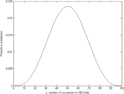
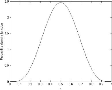
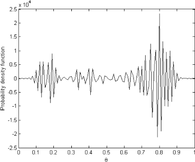
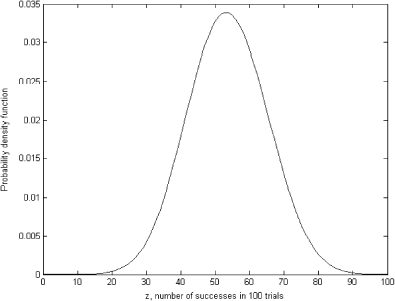
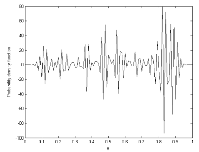
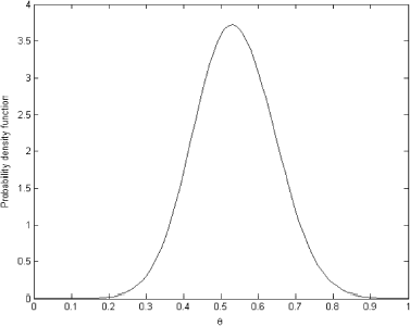
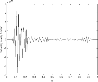
To obtain the predictive distribution in Fig. 1, we solved the forward problem (11) with prior distribution depicted in Fig. 2 as θ. The ordinary least squares (OLS) solution for the system (11) is presented in Fig. 3

FIGURE 3 OLS solution.

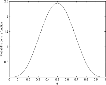
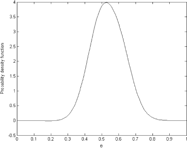
As we can see, the OLS solution is very oscillatory and makes no sense. It bears no resemblance to the exact known solution shown in Fig. 2. However, the regularized solution presented in Fig. 4 is very close to the exact one in Fig. 2 and can be used as the prior distribution.

FIGURE 4 Regularized solution.

We used the Morozov's discrepancy principle [6] to select regularization parameter λ = 8.5 × 10⁻⁵. However, the most interesting case represents a situation in which the predictive distribution is estimated from the data or from the prior knowledge, as in the case shown below.

Suppose we have some statistical data about the number of successes in 100 tosses in previous trials. We can use this historical data to estimate what can be called the empirical predictive distribution or marginal distribution, and using this distribution, we can solve for prior Eq. (9). The empirical predictive distribution being estimated from the data would contain a significant amount of noise, which would make the OLS solution of Eq. (9) very unstable and irrelevant. An example of the empirical prior distribution estimated from the data is shown in Fig. 5.

FIGURE 5 Marginal distribution.

The kernel density estimator, with a Gaussian kernel width of 10, was used to estimate this density from some historical data representing 5 trials of 100 tosses of a fair coin. The parameter of interest was the number of successes that was recorded as 61, 51, 60, 47, and 49 in simulations. As can be seen from Fig. 5, the marginal distribution of z is a bell shaped curve with mean value slightly higher than 50.

Due to the large kernel width used to estimate the density from the empirical data, the curve has one mode. Using this empirical density as the left hand side of Eq. (9), we can again numerically solve it for the prior distribution. The unregularized solution is shown in Fig. 6

FIGURE 6 Ordinary least squares solution.

As we can see, the solution is still very oscillatory and does not represent a real probability density function. However, the regularized solution depicted in Fig. 7 looks like a proper probability density and can be used as a prior for future inference.

FIGURE 7 Regularized solution.

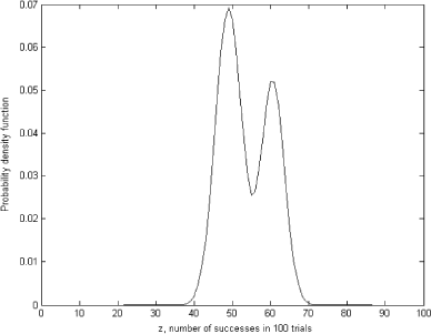
In this case, the most remarkable feature of using regularization is that it makes the inference about the possible prior distribution virtually insensitive to the ambiguous nature of the kernel density estimator. The problem with empirical density estimators is that their results are very sensitive to the chosen parameters of the techniques. For example, the density estimated with kernel techniques depends very much on the kernel width. Figure 8 shows the density of the same data set estimated with the kernel width chosen to be 3.

FIGURE 8 Marginal probability density function.

The estimated density now has two modes which looks quite plausible in the light of the available data. The OLS and regularized solutions are shown in Figs. 9 and 10.

FIGURE 9 OLS solution.

FIGURE 10 Regularized solution.

As can be seen from these figures, the OLS solution is again highly unreasonable and does not represent a real probability density function; however, the regularized solution is very close to the one obtained for the kernel width equal to 10 and shown in Fig. 7. The discrepancy principle was again used to choose the regularization parameters for these cases. It should be mentioned that in the last example, with the marginal distribution obtained from the data the first order, Tikhonov regularization was used with a smoothing operator representing an approximation of the first derivative.

3.2. Inference of Variance of Normal Distribution with Known Mean

The second numerical example to be analyzed is the inference about the variance of a normal distribution when the mean value is known. In this case the likelihood of future data z can be written as:

where μ is the known mean value. The corresponding conjugate prior density for variance is inverse-gamma and can be written as:

where α and β are two hyperparameters which define the shape and scale of prior distribution. Combining the likelihood and prior distribution we again obtain the prior predictive distribution:

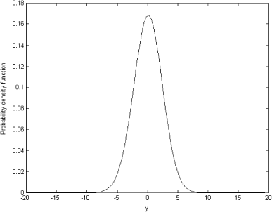
Now assume that we have a data sample y generated from N(μ,σ²). We can use this data sample to estimate the empirical distribution and use it as π(z|α,β). Having done this, we can again solve the integral equation (15) for the prior distribution π(σ²|α,β) using Tikhonov regularization. Suppose we have a data sample of ten random values generated from y ∼ N(0,1), y = (0.4855;−0.0050;−0.2762;1.2765;1.8634;−0.5226;0.1034; −0.8076;0.6804;−2.3646). The probability density function estimated from this sample is shown in Fig. 11.

FIGURE 11 Empirical marginal distribution.

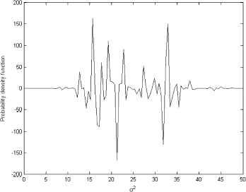
This probability density function is the only source of information about the random variable y that we have. The probability density function can be used as the empirical marginal distribution π(z|α,β) in the left-hand side of Eq. (15). Because the likelihood for the data is written in (13), we can numerically solve the integral Eq. (15). The OLS solution is shown in Fig. 12.

FIGURE 12 OLS solution.

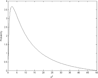
This solution cannot represent a real density function. However, the regularized solution is much more plausible and is very close to the inverse-gamma distribution. The regularized solution is shown in Fig. 13.

FIGURE 13 Regularized solution.

3.3. Practical Example. Estimating the Risk of Tumor in a Group of Rats

While evaluating drugs against cancer the experiments are usually performed on small animals like mice, rabbits or rats. The data for this example are borrowed from [7]. Suppose a current clinical experiment showed that 4 out 14 laboratory rats developed a tumor while receiving a zero dose of an anticancer drug. The problem is to estimate the probability of tumor in a population of rats using this current experiment, and historical data which reveals that in previous experiments the ratios of the rats which developed a tumor to the total amount of rats participating in the experiment were 5/49, 7/49, 12/49. Assuming the binomial model for the number of tumors and conjugate Beta prior B (α,β), we can use the method of moments to deduce prior Beta distribution from historical data. Using the following relationships between the parameters of Beta distribution and its moments

hence

and the prior distribution will be B (3.95, 20.27) which is depicted in Fig. 14.

FIGURE 14 Conjugate prior distribution.

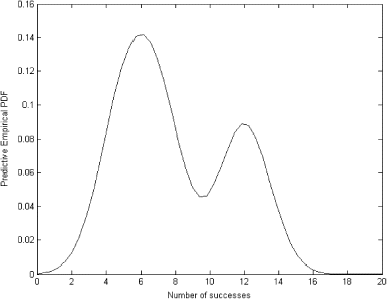
However, if we look at the historical data we can see that there should be two modes – one around 6, the other around 12. The empirical predictive distribution, which is estimated using historical data, is shown in Fig. 15. As expected it has two modes.

FIGURE 15 Empirical predictive distribution.

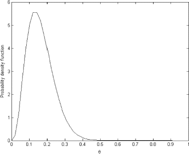
Using this empirical predictive distribution we can solve integral equation (7) to obtain prior distribution which is presented in Fig. 16.

FIGURE 16 Prior distribution on the probability of tumor obtained through the solution of integral equation.

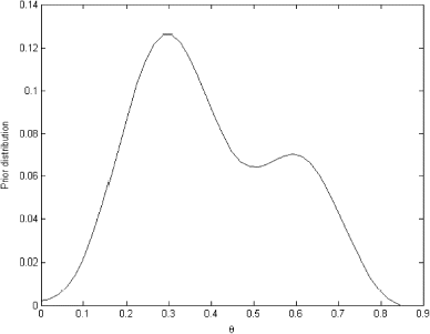
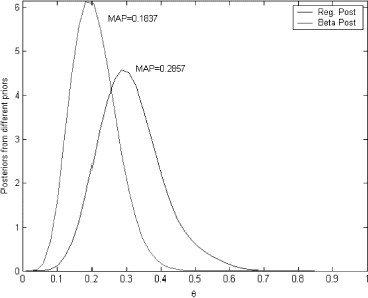
Now using the current data set – 4 out of 14 we can build a current likelihood function and obtain posterior probabilities for tumor to occur using two different prior – conjugate and the one selected using the proposed method. These two posterior probabilities are presented in Fig. 17.

FIGURE 17 Two posterior distributions obtained using two different priors.

As we can see these two posteriors differ significantly due to the differences in the priors. As the answer to this problem is unknown it is hard to argue that any of this solutions are closer to the “true” value; however, the maximum a posteriori (MAP) for the prior obtained through the solution of integral equation (0.2857) happened to be much closer to the probability obtained using current data 4/14 = 0.286.

4. Conclusions

This article presents a new inverse problem: inference of the prior distribution from the marginal or predictive distribution. The solution of this inverse problem requires the solution of the Fredholm integral equation of the first kind, which can be effectively solved using Tikhonov regularization. The assumption about the smoothness of the sought solution is very legitimate in this case because the sought solution is a probability density function, which must be smooth by its nature. Two numerical examples for the inference of the prior distribution for the parameter were given: first of a binomial distribution and then for inference of the variance of normal distribution with known mean. The described approach may represent a valuable alternative to the selection of prior in practical applications and provides new insight into the nature of prior selection. A practical example of the inference of probability of tumor in a group of rats is presented. The result is compared to a standard method of prior selection. Only a one dimensional case is analyzed. In multidimensional case we would have to obtain a prior for each individual parameter and then form the joint prior as a product of those individual priors using the argument about parameters independence.

Nomenclature

Table

L	=	likelihood function
π(θ|α)	=	prior distribution of the parameter
π(θ(x,α)	=	posterior distribution of the parameter
π(z|α)	=	prior predictive distribution
π(z(x,α)	=	posterior predictive distribution
θ	=	parameter of binomial distribution
λ	=	regularization parameter
α, β	=	hyperpameters
N	=	number of Bernoulli trials
z	=	random variable
x	=	random variable
μ, σ^2	=	parameters of normal distribution
B(α,β)	=	beta function

References

- Robert Christian P 1994 The Bayesian Choice. A Decision – Theoretic Motivation, Springer-Verlag New York
- Aitchison J Dunsmore IR 1975 Statistical Prediction Analysis, Cambridge University Press Cambridge
- Berger James O 1985 Statistical Decision Theory and Bayesian Analysis pp. 94–95 Springer New York
- MacKay , DJC . 1992 . Bayesian Interpolation . Neural Computation , 4 ( 3 ) : 415 – 447 .
- Tikhonov , AN . 1963 . Solution of incorrectly formulated problems and the regularization method . Doklady Akad. Nauk USSR , 151 : 501 – 504 .
- Morozov , VA . 1966 . On the solution of functional equations by the method of regularization . Soviet Math. Dokl. , 7 : 414 – 417 .
- Gelman A Carlin JB Stern HS Rubin DB 1995 Bayesian Data Analysis, Chapman & Hall London
- Turchin VF 1968 // USSR Comput. Math. and Math. Phys. 7 6 1962