Regularizing operators of real-valued inverse Laplace Transformation

Abstract

The article deals with presentation of a regularizing method of inverse Laplace transformation. The method allows us to obtain regularizing operators of inverse Laplace transformation. The considered approach allows us to find a connection between regularized and exact solutions, prove the convergence of the regularized solution to the exact one, and investigate the arising errors analytically. Provided error analysis reflects general features of any method of inversion of real-valued Laplace transforms. Only final step, i.e. evaluation of an integral of the convolution type, requires usage of numerical methods.

Keywords:

• Improperly posed problems
• Ill-posedness
• Tikhonov regularization
• Integral transforms numerical inversion
• Laplace transform inversion
• Mellin transform

1 Introduction

There are many problems of science and engineering that could be solved by means of Laplace transform. In the case when Laplace transform has been obtained by numerical calculations or from an experiment a numerical inversion becomes the only way to find the required solution.

Complexity of the problem depends on available initial information about a Laplace transform. D'Amore [3] states that in the complex case (i.e. the Laplace transform is explicitly given on its half-plane of convergence) the problem has been mainly solved by computing of the inversion integral. In real case (i.e. the Laplace transform is known on the real axis only) the Laplace inverse transformation is a well-known ill-posed problem (See, for example [19]).

The main approach in solving ill-conditioned problems is regularization [16]. However, direct numerical implementation of Tikhonov theory to the problem of inverse Laplace transformation turned out to be unsuccessful [17, 19]. After that several methods that used regularization were suggested [1–3,5,6,8,10].

At the present time in all known regularization methods of inverse Laplace transformation, the regularization step follows other transformations such as discretization or expansion of a Laplace transform or its original function into series. That is, a regularization is applied to a second-order problem, not to a problem of inverting of real-valued Laplace transforms itself. In this case it turns out to be impossible to determine restrictions and limitations of a proposed method differently than by carrying out an actual implementation of the method on a subset of Laplace transforms.

In this article Laplace inverse regularizing operators are obtained directly from the Laplace transformation definition. In the last section theoretical error analysis is given. It reveals advantages and limitations of the proposed method. Provided error analysis is consistent with well-known properties of Laplace transformation and reflects general features of any method of inversion of real-valued Laplace transforms.

This article presents a generalization of the method proposed by the author [12]. The cited paper provides rigorous proofs in case of k = 0 and examples of implementation of the method for inverting Laplace transforms, including the case of noisy data.

2 Outline of the inversion method

2.1 Inversion Formula

Consider the definition of Laplace transformation

as an integral equation of the first kind with respect to f(t). If a Laplace transform is analytic for , except p = 0, and parameter p is real and positive then Mellin transformation can be applied to Eq. (1):

where Γ(s) is gamma-function; are operator and parameter of Mellin transformation.

From the last equation we can find Mellin transform of unknown function as:

Inverse Mellin transform of does not exist. That is why Eq. (3) cannot be inverted and written in pre-image domain of Mellin transformation without specifying F(p). In other words, Laplace inverse operator does not exist if Laplace parameter p is real. It is worth mentioning that the same logic applied in case of Fourier sine or cosine transformations will lead us to exact inverse formulas.

The theory of ill-posed problem solving usually assumes the existence of inverse operator [16]. According to Tikhonov regularization theory in case of integral equations of the first kind of the convolution type we should multiply the right side of the Eq. (3) by a stabilizing factor. Using reasoning similar to [18] we will use a more analytical approach. Consider the following stabilizing factor:

where parameter R is a connected with regularization parameter α , k is an integer number.

After multiplying Eq. (3) by m(s,R) we get:

where f_R (t) is regularized solution.

It is apparent that as , and Eq. (5) tends to the exact Eq. (3). Rewriting the last equation in an equivalent form we get:

The inverse Mellin transform of m(s,α) can be obtained analytically:1

where .

Taking into account that for [4], we can find the inverse Mellin transform of Π(R, s) from Eq. (6):

As it can be seen integral in Eq. (8) converges if . Calculating integral (8) analytically using standard integral [15] we get:

where is generalized hypergeometric function.

Now when we have the function Π(R,x) we can invert Mellin transforms in Eq. (5) and obtain the formula for inverse Laplace transformation:

Conditions of convergence of integral (10) can be found using Eq. (9). Because of presence in (9) it can be rewritten as If then and . As a result integral (10) converges on the lower limit when

where parameter p is real.

Representing in terms of degenerate hypergeometric functions and using asymptotic expansion of the latter [13] we find that as and integral (10) converges on the upper limit if

Therefore, for each we have obtained the real-valued transfer function of Laplace inverse transformation. It is apparent from Eq. (9) that as , and does not exist for all x > 0. That is why Π(R,x) can hardly be evaluated numerically, without having a calculating formula.

2.2 Proof of Convergence

In terms of the suggested approach the connection between exact solution f(t) and regularized one f_R (t) can be found. Indeed, replacing in Eq. (5) with its expression from Eq. (2) we get:

Applying inverse Mellin transformation to the last equation we obtain:

It is apparent that integral (14) converges if an inverse Laplace transform f(t) is piecewise continuous for t > 0 and satisfies the following conditions:

The condition (15) corresponds to the previously obtained condition (12) in sense of expansion of an original function into power series. The relationship between conditions (16) and (11) is more complicated. In some cases it can be explained in terms of expansion of f(t) in asymptotic series [7].

Along with Eq. (14) we can find similar connection between regularized and exact Laplace transforms. Indeed, let be the Laplace transform of f_R (t):

where is operator of Laplace transformation.

Applying Mellin transformation to the latter we get equation similar to Eq. (2):

Replasing with its expression from (5) we obtain:

Inverting Mellin transforms in Eq. (19) the connection between functions F(p) and can be found:

As it should be expected integral (20) converges under conditions (11), (12) if parameter p is real and positive. In case of complex-valued parameter p integral (20) is convergent if (in addition) the Laplace transform F(p) is analytic for except for p = 0. Integral (20) is also convergent for if Laplace transform has isolated singular points on the imaginary axis of type , where 0 < r < 1.

It is interesting that functions F_R (p), F(p) and f_R (t), f(t) are connected with the same type of transformation. Equations (14) and (20) could be written in a form:

Integral (21) converges if function f(x) is piecewise continuous for x > 0 and satisfies the following conditions:

By analogy with Fourier integral theorem it can be strictly proved that if function f (x) is piecewise continuous, has piecewise continuous derivative for x > 0, and satisfies conditions (22), (23), then

The only change that we have to apply to the proof of Fourier integral theorem is usage of a different standard integral [15]:

As a corollary we have that if the original function is continuous and it satisfies conditions (15), (16). Respectively, as when Laplace transform obeys conditions (11), (12) and it is analytic for except for p = 0.

Let denote operator defined by Eqs. (9), (10), denote a subspace of inverse Laplace transforms that satisfy conditions (15), (16), and denote the corresponding subspace of Laplace transforms . The fact that operator is continuous with respect to F(p) is straightforward in case when . According to Tikhonov theorem [16, p. 49] the continuity of the operator and convergence of regularized solution to the exact one mean that operator from to is a regularizing operator of inverse Laplace transformation in Tikhonov sense.

According to the theory of ill-posed problem solving, each regularizing operator, under appropriate choise of regularization parameter that is coordinated with initial data inaccuracy, defines a stable method of approximated solution building. In particular this is true for the operator .

It is worth mentioning that all expressions above were obtained by formal usage of direct and inverse Mellin transformation. Furthermore, it can be explicitly shown that Laplace transformation of Eqs. (10) and (14) leads to Eq. (20) in both cases. Because of uniqueness of the Laplace transform this means that Eqs. (10) and (14) represent one and the same function f_R (t).

3 Error analysis

The fact that a regularized solution tends to the exact one when , i.e. under unbounded increase of input data accuracy, provides no information about the rate of convergence. We may assume that the rate of convergence depends on location and type of Laplace transform singular points. Equation (14) allows us to investigate errors analytically as well as the rate of convergence for an isolated singular point of F(p).

In practice for any given image function one should calculate the regularized solution f_R (t) by evaluating integral (10) with an appropriate value of parameter R. The optimal value of parameter R depends on inaccuracy of initial data. Because parameter R depends on parameter of regularization, its optimal value can be found with the help of known methods [9,16,17]. (See Tikhonov regularization method section in [11] for further references.)

In particular the method proposed by Glasko and Guschin [9] can be used in determining quasioptimal value of parameter R:

where

It is necessary to mention that this criterion has been proved only for some inverse problems. Therefore, its usefulness for discussed problem can be considered as a preliminary experimental result.

As a result of working with in-house developed software we can state that in case when a Laplace transform is known with three decimal digits, the optimal value of parameter R is approximately 3. The optimal value of R is not less than 10 when a Laplace transform can be calculated with double precision.

3.1 Singular Point is at the Origin

Consider the Laplace transform pair: , where r > 0. Due to conditions (15), (16) we have: . In this case Eq. (14) becomes:

Evaluating the last integral analytically [15] we will obtain a simple link between regularized and exact solutions:

As it is follows from Eq. (28) the regularized solution differs from the exact one only by a factor with a value close to 1. In case of R = 3 relative error equals approximately 0.05. If r is an integer number we have an interesting result: the regularized solution is independent of regularization parameter and . It is also worth mentioning that if an inverse Laplace transform has asymptotic function in form of power function, then that function can be determined using proposed method.

Using the symmetry property, integral (10) can be written in the following form:

Then for the Laplace transform we get:

Taking into account that in this case we conclude that

Equation (31) is true for any positive value of parameter R, that is why it is a good testing criteria for calculating f_R (t) using Eqs. (9), (10).

3.2 Singular Pointis in Left Half-plane

Consider the following Laplace transform pair:

In this case Eq. (14) will be

where .

Integral (33) converges if a > 0. Calculating the latter integral (standard integral, [15]) we get:

It is apparent that the first term of Eq. (34) tends rapidly to the exact solution f(t) as . The second term equals to zero if r is an integer (a is half-integer). In the case when r is a non-integer number and the second term increases with time.

The third term (in square brackets) of Eq. (34) is more complicated. Let z be . Then the third term of Eq. (34) can be written as:

Because of factor presence, the E₃ value is an alternating quantity. It is obvious that E₃ strongly depends on angle ϕ. For more precise analysis note that [13]

Then

Equation (37) shows that when and the decreasing rate of is highest, and it is getting slower as .

Obviously the quantity also depends on values of ρ and t. When we have the following estimation:

The factor vanishes as if a < 2. That is we can calculate an inverse Laplace transform with small relative error for small instances of time. If condition a < 2 is not satisfied, then relative error increases as or .

In case of applying analysis similar to the one used in Eq. (9) we can obtain asymptotic value for generalized hypergeometric function. As the result we found that the sum of all three terms of Eq. (34) tends to zero, that is as . In considered case , , so . Thus, we can calculate the inverse Laplace transform with small absolute error as .

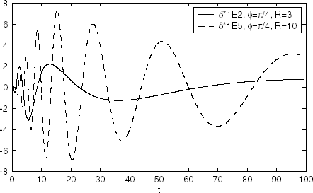
Figures 1 and 2 show graphs of real part of absolute error δ when , and . As it is seen from graphs the original function can be found with small absolute error for all instances of time. The absolute error value strongly depends on angle ϕ.

FIGURE 1 Real part of absolute errors for φ = 0.

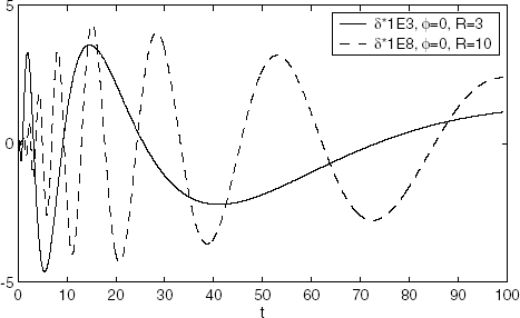
FIGURE 2 Real part of absolute errors for φ = π/4.

3.3 Singular Points are on the Imaginary Axis

It is also interesting to analyze the case when Laplace transform has a singular point on imaginary axis. Consider function . Then from Eq. (14) we have:

where .

Integral (39) is absolutely convergent if

Calculating integral (39) we will have:

When parameter R increases, the first term in Eq. (41) tends to the exact solution. The analysis of the second term is very similar to the previous case. Indeed, in this case instead of Eq. (37) we have:

That is second term decreases not slower than for any valid value . Thus, we have the slowest convergence to the exact solution as when Laplace transform singularities are on imaginary axis.

In case when , the second term tends to zero because . Therefore we can find the inverse Laplace transform with small relative error at the beginning of the process. If then as it was in the previous case. Then, if r < 1 we have that as . That is the final values of exact original function and f_R (t) are equal. However, if then does not exist and the values of the original function cannot be found as .

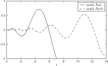
Graph in Fig. 3 shows absolute errors of restoration function sin t from its real-valued Laplace transform.

FIGURE 3 Absolute errors of restoration sin t from noisy real-valued Laplace transform.

4 Conclusion

The provided error analysis is consistent with the one given for convergence conditions of integral (20). It follows from the analysis above that, in case when conditions (11), (12) and others (specific to this method) are satisfied, we have that:

	if exists or f(t) has a power asymptotic function then f(t) can be approximately determined for all t>0;
	if does not exist then f(t) can only be approximately determined at the beginning of the process;
	regularized solution tends to the exact one when initial data inaccuracy tends to zero;
	the rate of convergence depends on location of the Laplace transform singular points. It is highest if singular points are on the negative real axis, and it is lowest if singular points are on the imaginary axis.

Provided error analysis allows us to conclude that the proposed method behaves in accordance with properties of Laplace transformation. Indeed, in case when does not exist the analysis above reveals the impossibility of determining values of such function as with the help of final-value or asymptotical expansion theorems of operational calculus [7].

The result that the rate of convergence strongly depends on singular points locations of the Laplace transform is consistent with results obtained by Orurk [14]. He has researched errors of the original function restoration when the Laplace transform is known only on the real axis.

Nomenclature

Table

F	=	Laplace transform
f	=	inverse Laplace transform
	=	generalized hypergeometric function
	=	direct and inverse Laplace operators
	=	regularizing Laplace inverse operator
	=	direct and inverse Mellin operators
m	=	stabilizing factor
p	=	Laplace parameter
R	=	conjugate parameter of regularization
s	=	Mellin parameter
t	=	time
α	=	parameter of regularization
Γ	=	gamma function
Π	=	transfer function

Subscripts

Table

R

=

regularized solution

Notes

¹Author was unable to find any specific references for Eq. (7). See Appendix.

Appendix

As it is known [4] an inverse Mellin transform corresponds to the pre-image function of two-sided Laplace transformation under substitution . Hence, we will first evaluate the pre-image function of the two-sided Laplace transformation. First, consider the case of k = 0:

where .

Then (7) will follow because of Mellin transformation property [4]:

Let us denote , then zeroes of the denominator of can be found from:

If α < 1 then , that gives . Then , and . The fact that results in n being an odd number, that is . Therefore . Hence, zeroes of the denominator are equal to , where . Therefore the function has poles at , with residues as follows:

where upper sign corresponds to the upper complex half-plane, and lower sign corresponds to the lower one. For , we can find the original function of two-sided Laplace transform when t > 0 by evaluating complex integral along the contour closed in the left half-plane:

Finally substituting and having in mind that the sum in the last expression is a simple geometric progression we will obtain the inverse Mellin transform for :

The same result can be obtained for x > 1, t < 0 by calculating complex integral along the contour closed in the right half-plane.

References

- d'Alessio , A. , D'Amore , L. and Laccetti , G. 1993 . First results about Tikhonov regularization methods for numerical inverting a Laplace transform function . Rend. Acad. Sci. Fis. Mat., Napoli , 4 : 60, 75
- Al-Shuaibi , A. 1997 . On the inversion of the Laplace transform by use of a regularized displacement operator . Inverse Problems , 13 : 1153
- D'Amore L. Murli A. Rizzardi M. 1996 A computational algorithm for the real inversion of a Laplace transform function Abstract of the Int. Conf. on Inverse and Ill-posed Problems Moscow
- Bateman H. Erdelyi A. 1954 Tables of Integral Transforms McGraw-Hill New York
- Brianzi , P. and Frontini , M. 1991 . On regularized inversion of the Laplace transform . Inverse Problems , 7 : 355
- Chauveau , D.E. , van Rooij , A.C.M and Ruymgaart , F.H. 1994 . Regularized inversion of noisy Laplace transforms . Adv. Appl. Math. , 15 : 186
- Ditkin V.A. Prudnikov A.P. 1965 Integral Transforms and Operational Calculus Pergamon Press New York
- Dong , C.W. 1993 . A regularization method for numerical inversion of the Laplace transform . SIAM J. Numer. Anal. , 30 : 759
- Glasko , V.B. and Guschin , G.V. 1966 . About Tikhonov regularization method in solving of nonlinear equations . Vychisl. Met. Progr. , 5 : 61
- Iqbal , M. 1997 . On spline regularized inversion of noisy Laplace transforms . J. Comput. Appl. Math. , 83 : 39
- Istratov , A.A. and Vyvenko , O.F. 1999 . Exponential analysis in physical phenomena . Rev. Sci. Instrum. , 7 : 1233
- Kryzhniy , V.V. 2003 . Direct regularization of inversion of real-valued Laplace transforms . Inverse problems , 19 : 573
- National Bureau of Standards 1964 Handbook of Mathematical Functions (Applied Math. Series 55) Pitman Boston MA
- Orurk I.A. 1965 New Methods of Synthesis of Linear and Some Nonlinear Dynamical Systems Nauka Moscow-Leningrad
- Prudnikov A.P. Brychkov Yu.A. Marichev O.I. 1981 Integrals and Series Nauka Moscow
- Tikhonov A.N. Arsenin V.Y. 1977 Solutions of Ill-posed Problems Winston and Sons Washington D C
- Tikhonov , A.N. and Glasko , V.B. 1964 . About approximate solution of Fredholm integral equations of the first kind . Zh. Vychisl. Mat. Mat. Fiz. , 4 : 564
- Trofimov , A.S. and Kryzhnii(y) , V.V. 1994 . Reconstruction of nonstationary temperatures from the results of measurment on a heat-insulated wall surface . J. Eng. Phys. Thermophys. , 67 : 1113
- Zaikin , P.N. 1968 . About numerical solution of operational calculus inverse problem . Zh. Vychisl. Mat. Mat. Fiz. , 8 : 411
Appendix
As it is known [Citation4] an inverse Mellin transform corresponds to the pre-image function of two-sided Laplace transformation under substitution . Hence, we will first evaluate the pre-image function of the two-sided Laplace transformation. First, consider the case of k = 0: