Inversion of spectroscopic data, application on CO₂ radiation of flame combustion

Abstract

This article deals with the inversion of spectroscopic measurements to obtain temperature and concentration profiles of a gas. The Radiative Transfer Equation (RTE) is discretized as a one-dimensional equation to simulate a spectrum and adjoint state method is used to compute the sensitivity matrix. The Singular Value Decomposition of the sensitivity matrix enables analyzing information content of a spectrum, and defining the number of retrievable parameters for a noise level. This number and the rank of the sensitivity matrix indicate the difficulty of data inversion. When inversion seems difficult, regularization is necessary and information about profiles is included using parameterization. This method is applied on CO₂ radiation, where inversion of simulated data for Gaussian distributions is studied to know what to do with real case data. Finally, real case inversion is performed for spectroscopic measurements carried out on the exhaust of a motor.

Keywords:

• Parameter estimation
• Sensitivity analysis
• Parameterization
• Radiative transfer equation
• 2000 Mathematics Subject Classifications: 49J15
• 90C31
• 15A18

1. Introduction

There are several studies about the inversion of the Radiative Transfer Equation (RTE) in order to find temperature distribution and some medium characteristics, or to calculate some source properties for industrial or ecological purpose. In the literature, efforts have been reported on the reconstruction of flame temperature. Determining gas distribution is an additional requirement to be pulled out from spectroscopic data. We cite here Yousefian et al. [4,5] who have used infrared emission to retrieve temperature and concentration profiles for moderately noisy measurements in axisymmetric flames by Abel Inversion. Liu et al. [10,12] worked on the estimation of temperature, spectral absorption coefficient, source-term distribution in a non-grey medium. Measuring temperature in order to retrieve some radiative parameters is the subject of other works like Park and Yoon [8,9].

The accumulation of high-resolution spectroscopic data motivates the use of more generic methods that can be applied for various wave numbers, instrument resolutions, and molecules in a gas. Here we present a tool to study the influence, on radiation intensity, of temperatures and concentrations of a molecule in a gas, and how to use their influence to retrieve their distributions in the observed medium. An application on CO₂ radiation is given for both the simulated data and real case data.

To study this phenomenon, the main hypotheses proposed for the physical model are local thermal stability and establishment of temperature and concentration profiles. Additional simplifying hypotheses, related to a first-order approximation of the real behavior of a flame gas, are made here. They consist of considering the gas real index as equal to one and neglecting all the following: the particles emission absorption (for example soot's particles), the reflection at the air–gas interface and the scattering effect compared with the emission–absorption one.

Since the numerical resolution of the one-dimensional RTE is very fast on modern computers, then numerical efficiency is not the main issue here, and the differential formulation of RTE is chosen, for its simplicity, to simulate spectroscopic data. A very important question rarely answered is evaluating, before inversion, the number of parameters which can be extracted from a given set of spectroscopic measurements. We address this problem by performing the singular value decomposition SVD of the Jacobian matrix [1–3,6], where data sensitivity to parameters variation is analyzed and a definition of the number of retrievable parameters for a noise level is given. Jacobian is computed, using an adjoint state technique, at a cost independent of the number of unknown parameters (it depends only on the discretization of the RTE). Gaussian distribution is chosen for both temperature and concentration profiles to apply this method on simulated data related to CO₂ spectrum. Results of this application enables understanding and the ability to decide what to do for real case data.

The CO₂ spectrum radiation is studied between 2379 and 2397 cm⁻¹, which is in the range of high sensitivity with respect to the temperature, so we hope for a good estimation and stability of the temperature's parameters.

We estimate the temperature and concentration profiles by minimizing the misfit of the modeled spectrum to the measured spectrum, using the trust region method, where linearized problems are solved by the Gauss–Newton algorithm, and linear systems are solved by the conjugate gradient method.

2. Direct and inverse problem for RTE

For the previous hypotheses the radiation intensity L_σ(x) measured at a point x emitted by the quantity of gas situated at the left of x (see figure 1) depends on distributions between 0 and x of temperature T and concentration C of the studied gas.

Figure 1. The observation of radiation intensity.

This dependence is expressed by the following differential equation: (---219--1) (---219--2) where

1.	K σ (T,C) is the monochromatic absorption coefficient of the gas for a wave number σ at temperature T and concentration C. This coefficient is expressed by: (---219--3) here, P is the pressure, k is Boltzman constant, and the coefficients (---219----1) depend on the wave number σ and they are considered as known for our study. They are obtained by a modelization study of Kσ run over a high-resolution spectroscopic database HITEMP [11].
2.	(---219----2) is the black body emission expressed by Planck's law: (---219--4) the values of k1 and k2 are given in the nomenclature.
3.	The initial value, Lσ , 0 represents the background radiation for the wave number σ. In this article, there is no background radiation, so its value is null.

We measure, by a detector located at x = d, the radiation intensity (---219----3) resulting from absorption and emission by the gas situated to the left of x = d, see figure 1. The wave number σ is in a given set of wave numbers Σ covering the spectrum of interest. For every wave number σ ∈ Σ, temperature profile T and concentration profile C, we compute the solution L_σ of the differential equation (1)(---219--1) for the initial condition L_σ 0 = 0. We denote the radiation intensity L_σ(d) computed at x = d by: (---219--5) So we have to solve the following non-linear equations:

Find the two profiles that satisfy: (---219--6) The least squares formulation of this problem is the minimization problem: (---219--7) If we assume that T and C profiles are in the space (---219----4) of continuous functions over [0,d], then their space is infinite-dimensional space: this fact compared to the finite number of data shows the ill-posedness nature of this problem where clearly there is no uniqueness neither stability of the solution. Consequently regularization is necessary, where a priori information about profiles is used. This a priori information is a fixed shape for both of functions T and C, parameterized by ‘few’ parameters. But first we have to discretize the RTE, and perform sensitivity analysis to have an idea about the difficulty of this inverse problem.

3. Discretization and sensitivity analysis

For a wave number σ ∈ Σ, and two distributions T and C in [0,d] for temperature and concentration respectively we want to evaluate (---219----5) defined in (5)(---219--5) . Let (---219----6) be a uniform subdivision of the segment [0,d] with a step of h=d/N, and we associate to this subdivision the following piecewise constant approximations for temperature and concentration profiles, which are denoted by: (---219--8) (---219--9) The searched discrete profiles are then in finite-dimensional space of dimension 2N. The radiative intensity L_σ , evaluated at the discretization points (---219----7) , gives the following vector: (---219--10)

To evaluate L, the simplest explicit Euler scheme is chosen for the resolution of the differential equations (1)(---219--1) and (2)(---219--2) . This resolution gives the following state equations: (---219--11) (---219--12) (---219--13) and (---219--14)

The scheme (14)(---219--14) is of order one with respect to h, so a small value for h is necessary to have a good precision on the discrete solution L as an approximation of the solution of (1)(---219--1) . This scheme is stable under the condition: (---219--15) which must be satisfied in the numerical tests. Once the recurrence system (14)(---219--14) is solved, the discrete value, noticed as well by (---219----8) , is given by: (---219--16) Consequently, for the wave number σ, the following discrete forward map is perfectly defined: (---219--17)

The gradient of (---219----9) with respect to the 2N-dimensional vectors (T, C) is computed by an adjoint state technique (see Appendix A). First the adjoint equation has to be solved: (---219--18) (---219--19) (---219--20) (---219--21) then derivatives with respect to piecewise constant distributions (8)(---219--8) and (9)(---219--9) can be expressed as: (---219--22) (---219--23)

Since temperatures and concentrations are of different scales, which influences the sensitivity study, then adimensionalized variables have to be used to reduce this effect. We denote the new adimensionalized distributions by: (---219--24) where the values of T_m and C_m are in our case: (---219--25)

The new application: (---219--26) is denoted by (---219----10) as well, and we specify the variable when it is necessary to avoid confusion. Its derivatives are: (---219--27) we denote by (---219----11) the line vector of these derivatives. The simulated spectrum for all wave numbers of Σ is defined as: (---219--28) whose derivatives give the sensitivity matrix of the spectrum, denoted by: (---219--29)

The main tool used to study sensitivity is the Singular Value Decomposition (SVD) of the sensitivity matrix [2], it gives: (---219--30) In this expression (---219----12) are the right singular vectors in the parameter space, (---219----13) are the left ones, where I is the number of wave numbers in Σ, Λ contains the singular values of (---219----14) , which are positive here, in a decreasing order. For a singular value λ, if we denote by v_λ and u_λ the corresponding right singular vector and the left one, we can write: (---219--31)

When λ is non-zero, parameters variations in the direction v_λ imply variations in measurements in the direction u_λ of modulus λ. So the rank of the sensitivity matrix, which equals the number of non-null singular values, indicates the amount of ‘independent’ or ‘non-correlated’ information about parameters contained in the measurements. But a small singular value λ implies a small effect in measurements space. This effect may be easily hidden by noise in measurements, thus making it impossible to retrieve the component of the parameter in the corresponding singular direction u_λ. In the following section the number of retrievable parameters is defined for a given noise level; it indicates the difficulty of the inversion of the corresponding data.

4. The number of retrievable parameters

In this section, the techniques used and their results are written for adimensionalized parameters. The way to generalize these results for another type of parameterization is described at the end of the section.

We assume that the measured spectrum (---219----15) is a perturbation of the true spectrum (---219----16) : (---219--32) where δL accounts for the noise. When the model is perfect to represent the reality, we can write for true distributions t₀,c₀): (---219--33)

Here we assume that the model is perfect then this hypothesis holds clearly for simulated data. For real case data, if the model is not really good, then inversion may guide modelization effort to get a better model to represent the reality.

We want to investigate in how many independent directions the parameters t and c can be confidently retrieved from the noisy data (---219----17) . For this purpose we linearize the forward model at t₀, c₀) and perform the SVD of (---219----18) , which amounts to consider that parameters variations (δ t ,δ c) are a minimizer of the quadratic function: (---219--34) The decomposition of (δ t,δ c) on the basis of right singular vectors V gives: (---219--35) The decomposition of δL on the left singular vectors U gives: (---219--36) If the noise δL has a null component on the image of the linear application (---219----19) then the minimizer of J_lin is the null vector, and consequently there is no effect of the noise on the solution. We consider then that δL is in the image of (---219----20) to study its effect. In this case, if we denote by N_K the rank of the sensitivity matrix, then the minimizer of J_lin is immediately given by: (---219--37) where λ_i is the ith singular value of the sensitivity matrix, so that: (---219--38)

This inequality controls the absolute value of the error in the estimated parameters. The controlling factor 1/λ_i explodes for little values of λ_i ; in this case we do not really control errors of estimated parameters. On the other hand, it is interesting to try to control the relative errors of the parameters. For this purpose we need to check some properties of the forward application (---219----21) as convexity. Because the forward model is defined by an intermediate resolution of a differential equation, its convexity cannot be shown directly: we discussed in Appendix B how to check this property numerically over a segment. The result (B.6)(---219--0-6) written at the point (t₀,c₀) gives: (---219--39) Combining (38)(---219--38) and (39)(---219--39) gives: (---219--40) this means that the error on the ith parameter obtained by inversion is controlled by the error on the measurements amplified by the ratio λ₁/λ_i ≥1. For an upper bound ε of the relative errors on measurements: (---219--41) the parameter a_i is called retrievable if it satisfies λ_i/λ₁> ε. This implies: (---219--42) We call N_r(ε) the number of retrievable parameters for a noise level ε. Notice that N_r(0) is the rank N_K of the Jacobian (---219----22) . These two numbers, compared to the number of parameters N_p, give a quantitative idea of the difficulty of the inversion problem at hand.

We notice that the number N_r(ε) is evaluated by model linearization at a given point. For non-linear inverse problems, Jacobian differs from one point to another, so the value of N_r(ε) is local. When N_r(ε ) and N_r(0) are evaluated at true profiles (t₀,c₀) generating the simulated data (---219----23) satisfying (33)(---219--33) , then they indicate the difficulty to retrieve profiles (t₀,c₀) by inversion of the noisy data (---219----24) of (32)(---219--32) .

For adimensionalized parameters and for the example considered in the next section, we will see that N_r(ε) and N_r(0) have small values compared to N_p =12N; consequently we cannot hope that retrieving all the parameters, and regularization is necessary.

Regularization by parameterization is considered to be a good way to include information about profiles in the inversion process. Parameterization consists in searching for the temperature and concentration profiles as closed-form formula depending only on a small number of parameters whose values have to be deduced by minimizing differences between initial simulated data and objective data. Parameterization is performed by specifying an application Φ that associates temperature and concentration distributions (t ,c ) to a vector of all unknown parameters p. When applied to the problem (7)(---219--7) , it gives: (---219--43) This ‘new’ inverse problem can be studied by the same manner as the original problem. We can define for a noise level the number of retrievable parameters for the new parameterization and compute N_r(ε) and N_r(0) in order to have an idea about the corresponding inversion difficulty. If inversion seems not very difficult, then optimization with respect to p of the objective function (43)(---219--43) may give a satisfactory result.

As for the optimization algorithm, a trust region reflective method was used here for its good performance. In this method, a local quadratic approximation of the objective function is minimized over a region called the trust region. This region depends on problem constraints and the non-linearity of the objective function. To minimize this quadratic approximation Gauss–Newton and Conjugate Gradient algorithms are the main tools used inside iterations [7].

Finally, we notice that results of sensitivity, difficulty evaluation using N_r(ε) and N_r(0), and optimization are related to the choice of the set of wave numbers Σ. We check some of these properties for several subsets of wave numbers and compare information content and efficiency of the corresponding measurements to retrieve profiles for given noise levels. This could be useful in designing the measurement device, where getting the maximum of useful information with the lowest price is a crucial issue. In the numerical study, a comparison of four subsets of wave numbers is given to illustrate this idea, and we think that the result may interest designers and users of spectroscopic devices.

5. Application on synthetic data for CO₂ radiation

In this section we apply results of previous sections on CO₂ emission–absorption simulated spectrum. Our objective here is to understand what may happen for real case data inversion. Using simulated data is equivalent to saying that the physical model is perfect to describe the reality, and in this case the hypothesis (33)(---219--33) holds. The radiative properties of CO₂ for wave numbers of a set Σ are given as a table of coefficients (---219----25) used to compute K_σ for all wave numbers. The Gaussian distributions for temperature and CO₂ concentration are assumed here. Experts believe that these distributions could represent approximately what the studied motor, in the real case example, can produce as temperature or CO₂ concentration during its activity cycle.

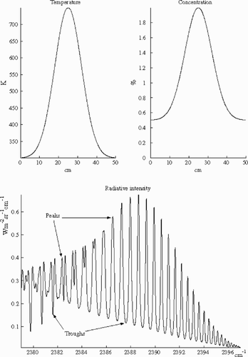
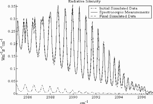
We discretize the space domain [0,d] in 200 segments, in a way that it satisfies the stability condition (15)(---219--15) , and we resolve the differential equation (1)(---219--1) . With this discretization, temperature and concentration profiles are described by 200 values per profile, then we have N_p = 400. The set of all wave numbers Σ contains 901 equidistant wave numbers between 2379 and 2397 cm^− 1 .The simulated spectrum for Σ and Gaussian distributions for temperature and concentration, are shown in figure 2.

Figure 2. Radiative intensity for Gaussian distributions, and some subsets of wave numbers.

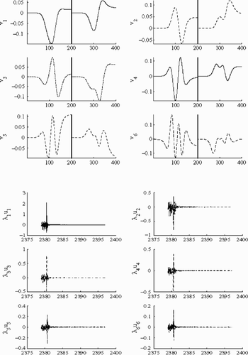
Sensitivity matrix for adimensionalized parameters (t₀,c₀) is computed, and the SVD of this matrix is performed. We plot singular vectors in order to have an idea about sensitivity of radiative intensities with respect to discretization values of temperature and concentration. Figure 3 shows the first six right singular vectors (---219----26) and their corresponding images (---219----27) by the sensitivity matrix.

Figure 3. The first six right singular vectors and their images by the sensitivity matrix.

Every right singular vector has its first 200 components in the adimensionalized temperature space, and has the last 200 components in the adimensionalized concentration space. The part of the first right singular vector in the adimensionalized temperature space looks like the temperature profile. This is not the case for the part of this vector in adimensionalized concentration space. Since this vector corresponds to the greatest singular value, a good sensitivity for temperature distribution can be deduced. Images of the first six right singular vectors have small components for wave numbers in [2385 cm⁻¹,2397 cm ⁻¹], then radiative intensities that may give information about temperature and concentration distributions are mainly those situated in [2379 cm⁻¹, 2385 cm⁻¹]. We can see clearly that λ₁ u₁ has the largest component in measurements space, that shows clearly the high sensitivity of measurements for parameter variations in the direction of the first right singular vector.

On the spectrum of figure 2, some subsets of wave numbers are distinguished; they correspond to local minima or maxima of radiative intensity. Besides the set of all wave numbers Σ, three subsets of wave number were specified here:

1.	The set of the 46 wave numbers of ‘Peaks’ corresponding to local maxima of spectrum intensity – it is denoted by Σ1.
2.	The set of the 47 wave numbers of ‘Troughs’ corresponding to chosen local minima of radiation intensity, denoted by Σ2.
3.	The mixed set of 93 wave numbers of Peaks and Troughs denoted by Σ3.

We will check the inversion difficulty for these four sets of wave numbers by evaluating the corresponding N_r(0) and N_r(ε) for the noise level ε =1%. For this purpose we compare in figure 4 the curve of  − 20 log₁₀(λ_j/λ₁ ) to the line  − 20 log₁₀ε. Evaluating the indicators N_r(0) and N_r(ε) for all subsets of wave numbers gives:

1.	For the set of Peaks Σ1, we have Nr(ε )=5 and Nr(0)=46.
2.	For the set of Troughs Σ2, we have Nr(ε )=6 and Nr(0)=46.
3.	For the set of Peaks and Troughs Σ3, Nr(ε )=6 and Nr(0)=56.
4.	For all wave numbers Σ, Nr(ε )=6 and Nr(0)=58.

Figure 4. Evaluation of N_r(1% ) corresponding to adimensionalized parameters for four subsets of wave numbers.

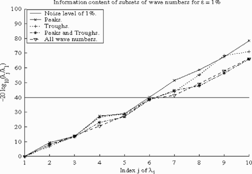
We noticed that the difficulty of inversion expressed by the factors N_r(0) and N_r(ε) has nearly the same order for the two subsets Σ and Σ₃. If we notice that in Σ₃ there are only 93 wave numbers, compared with 901 for Σ, then we can say that the set Σ₃ contains almost all the information of the spectrum about parameters. Then using Σ₃ can be an option to reduce measurement cost without losing a lot of their information content. Since designing devices is not our main objective here, we will use for inversion the set of all wave numbers Σ containing all information about parameters.

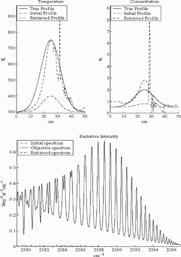
For all wave numbers Σ, the values N_r(ε )=6 and N_r(0)=58 compared with the total number of parameters N_p = 400 shows that inversion is difficult, and estimating all parameters seems hopeless. We also checked what the inversion of the simulated data (---219----28) of figure 2 may give. We see in figure 5 the reconstructed profiles together with the true ones; they are very different despite the fact that they produce the same desired spectrum.

Figure 5. Inversion result of retrieving all discretization values of profiles.

Then to obtain uniqueness, it is necessary to regularize the problem by using information about the possible shape of profiles. We suppose that the searched distributions are Gaussian, which is the case for the objective simulated data (---219----29) of figure 2, and we parameterize them using the following formulas: (---219--44) (---219--45) Sometimes one has a good estimation of t_∞ and c_∞ , and they can be considered as the boundary values for their distributions. In such a case, we use a sub-parameterization by freezing the values of t_∞ and c_∞ and searching values for the remaining ones. The localization of the maximal temperature and maximal concentration values enables freezing the values of x_t and x_c. Here is a recapitulation of all the fixed values: (---219--46) The new reduced parameterization is defined by: (---219--47) By the same way used to deduce the inequality (39)(---219--39) , we can have a similar inequality for the new parameterization obtained at the objective point p₀ which satisfies: (---219--48)

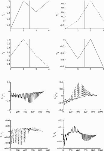
The SVD of the sensitivity matrix (---219----30) shows the influence of parameter variations on measurements. In figure 6 we see that the first right singular vector has its main component on the direction of t_max then measurements are the most sensitive to this parameter, and we expect that it may be retrieved with the best precision.

Figure 6. The four right singular vectors and their images by the sensitivity matrix.

By checking the inequality (39)(---219--39) for the new parameterization Φ, by the same way as it was done for the adimensionlized parameterization, we define indicators of inversion difficulty N_r(0) and N_r(ε) for a given noise level ε. These indicators are estimated for the previous four sets of wave numbers (see figure 7). We have N_r(ε )=2 and N_r(0)=4 for all of the subsets: this means that at least a half of parameters can be retrieved for a noise level of 1% in measurements, and at most all of them will be retrieved (it was not the case for adimensionalized parameters). This interpretation is the same for all subsets of wave numbers. Then inversion for the new parameterization is more hopeful than inversion for the adimensionalized parameterization. In fact, a priori information on the Gaussian shape of profiles eliminates the kernel and small singular values of the Jacobian of the forward model. Since noise exists in real case measurements, it is necessary to perform inversion on simulated data including noise, and evaluate the noise effect on retrieving parameters. The considered noise is generated by a random uniform generator with maximum value γ. For the considered simulated spectrum (---219----31) of maximal radiation intensity L_max , the noise corresponding to a noise level ε is the noise of maximal amplitude of γ =ε L_max. Three noise levels are tested: 1, 10, and 20%. For each noise level, different uniform random noises are generated and inversion is performed to retrieve parameters. We content ourselves by generating 14 different random noises for every noise level. The averaged values of parameters and the averaged relative error are given in table 1.

Figure 7. Evaluation of N_r(1% ) corresponding to the subparameterization Φ for four subsets of wave numbers.

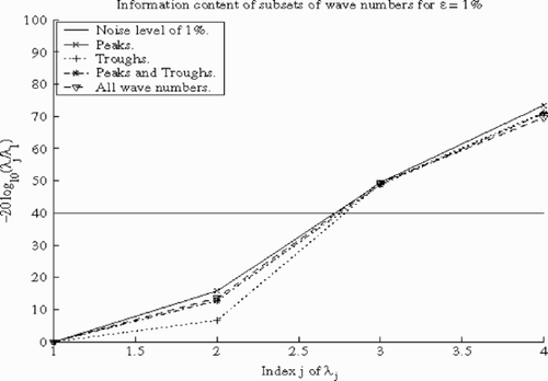
Table 1. Averaged values and averaged relative errors for different noise levels.

	Noise level	Tm ×tmax	αt	Cm×cmax	αc
	(%)	(K)	(cm)	(%)	(cm)
Real values p0	–	750	10	2	10
Initial values	–	490	7	1.4	7
Averaged values	1	749.754	9.913	2.024	9.881
	10	748.933	9.738	2.144	9.762
	20	750.779	10.58	1.992	11.282
Averaged relative	1	0.0739	1.409	1.859	1.975
error (%)	10	0.6255	13.211	19.815	18.725
	20	0.8127	18.611	24.040	30.4019

We noticed first that the averaged values are close to real values, but their quality is expressed by the averaged relative error, where we see clearly that for high noise levels in measurements the relative error on retrieved parameters increases. These results confirm the sensitivity analysis conclusion where we see that t_max has been retrieved with a good precision and has a good stability with respect to noise level, α_t comes after, while the values of concentration parameters have less precision.

The previous study was done for other shapes of temperature and concentration profiles, where we noticed that generally we did not have sufficient information in spectroscopic measurements to retrieve all discretization values for researched distributions. Then parameterizing the profiles seemed to be efficient as a regularization method for this inversion problem.

Now we can deal with real data where we use the sub-parameterization of temperature and CO₂ concentration profiles to regularize the ill-posed problem.

6. Application on real case data

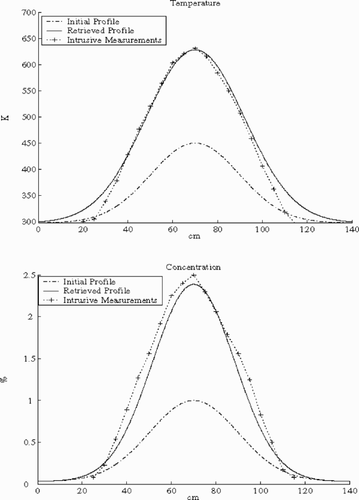
Two kinds of measurements were carried out on the exhaust of Rolls–Royce Spey at DeRA, intrusive measurements and spectroscopic measurements (non-intrusive measurements). We have worked on the spectroscopic data to retrieve temperature and CO₂ concentration using the previous method. Profiles were supposed, by experts of motors, to be Gaussian profiles, and they believe that Gaussian shape can describe the unknown distributions sufficiently .

We consider here the sub-parameterization defined in (47)(---219--47) where the main parameters to be retrieved are: (---219---1) Minimizing the corresponding objective function (43)(---219--43) to spectral measurements, shown in figure 9, gives profiles shown in figure 8.

Figure 8. Temperature and concentration profiles for real case inversion.

Figure 9. Inversion CO₂ spectrum of the exhaust of a motor.

The results of the intrusive measurements are shown in order to be compared with inversion results. We do not believe here that intrusive measurements are more accurate than inversion results; neither do we believe that inversion results are more reliable than intrusive measurements. We just notice that they have close values, and this fact gives confidence in both of them. This confidence assures us that the considered model is good enough to describe the reality.

7. Conclusion

Inversion of spectroscopic data to obtain temperature and concentration distributions is an ill-posed problem. Evaluating the rank of the sensitivity matrix and the number of retrievable parameters for a noise level motivates using parameterization of profiles as a regularization technique.

Applying this method on CO₂ radiation simulated spectrum in the zone [2379 cm⁻¹, 2397 cm⁻¹] for Gaussian distributions, enables retrieving temperature and concentration profiles for low noise levels. We notice that for high noise levels the maximal temperature value is more stable than other parameters and temperature parameters are more stable than concentration ones. With real case data, the inversion results are very close to intrusive measurements, this ensures confidence in inversion algorithm.

Nomenclature

Table

C=	Concentration (%)
h=	Length of a segment (cm)
JΣ=	Objective function
k=	Boltzman constant, k=1.38 e^−23 (J K^−1)
k1=	Constant in Planck's Law, k1=1.19 e^−8 (W cm^3)
k2=	Constant in Planck's Law, k2=1.438 (cm K)
Kσ =	Absorption coefficient for σ (cm^−1)
Lσ, 0=	Background Radiation (W m^−2,sr^−1,cm^−1)
Lσ =	Radiative intensity for σ (W m^−2,sr^−1,cm^−1)
(---219----40) =	Measured intensity for σ (W m^−2,sr^−1,cm^−1)
(---219----41) =	Vector of (---219----42) for all σ ∈ Σ
(---219----43) =	Computed intensity for σ (W m^−2,sr^−1,cm^−1)
(---219----44) =	Vector of (---219----45) for all σ ∈ Σ
(---219----46) =	Local Planck function for σ (W m^−2,sr^−1,cm^−1)
N=	Number of subsegments
P=	Pressure (bar)
T=	Temperature distribution (K)
u=	State variable
(---219----47) =	Adjoint state variable
Φσ =	Lagrangian function for σ
σ=	Wave number (cm^−1)
Σ=	A set of wave numbers

Acknowledgment

We acknowledge here DeRA for their results of intrusive measurements, and the Auxitrol company for its support.

Appendix A: Derivatives formula

We define the Lagrangian function: (---219--0-1) where (---219--0-2) is called the state vector, and (---219--0-3) is called the adjoint vector (or Lagrange vector).

For temperature and concentration profiles (T ,C), we denote by K(T ,C), L⁰(T) and L (T ,C), the solution vectors of state equations (11)(---219--11) –(14)(---219--14) respectively. Let u(T, C) be the corresponding state vector: (---219--0-4) we notice that: (---219--0-5) Let (---219----32) be the vector that satisfies: (---219--0-6) This equation leads directly to the system (18)(---219--18) –(21)(---219--21) defining the adjoint vector (---219----33) . Then derivatives of (---219----34) are given by: (---219--0-7) (---219--0-8) this gives: (---219--0-9) (---219--0-10) which gives (22)(---219--22) and (23)(---219--23) .

Appendix B: Convexity numerical check

For a real value b we denote by b the homogenous profile of all components equal to b. We establish here the formula (39)(---219--39) . It follows from the fact that (---219----35) appears to be convex (for all wave numbers) over the segment started by the homogenous profiles (0.3,0) and finished at (t₀,c₀), as we can see in the figure 10.

Figure 10. Convexity over the segment between (t₀,c₀) and (0.3,0) of radiative intensities for all wave numbers σ ∈ Σ.

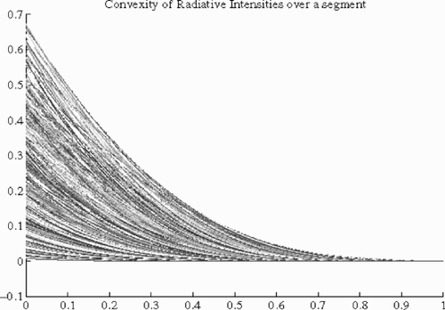
This convexity, shown numerically, implies: (---219--0-1) The resolution of RTE (1)(---219--1) –(3)(---219--3) for c =0 gives clearly (---219----37) . Hence (B.1)(---219--0-1) becomes: (---219--0-2) This implies for all the spectra: (---219--0-3) and as it is t₀ ≥ 0.3: (---219--0-4) But (---219--0-5) where λ₁ is the greatest singular value of (---219----38) , then: (---219--0-6) Finally to obtain (39)(---219--39) we notice that (---219----39) .