Near real-time atmospheric contamination source identification by an optimization-based inverse method

Abstract

In this article, we propose a method to identify contamination events (location and time of release) by enhancing a mathematical method originally proposed by Carasso et al. (Carasso, A., Sanderson, J.G. and Hyman, J.M., 1978, Digital removal of random media image degradation by solving the diffusion equation backward in time. SIAM Journal of Numerical Analysis, 15(4)). The method of the Marching-Jury Backward Beam/Plate Equation, applied earlier to groundwater problems, is enhanced and coupled to discrete Fourier transform processing techniques to solve a two-dimensional (2D) advection-dispersion transport problem with homogeneous and isotropic parameters backwards in time. (Atmadja, J. and Bagtzoglou, A.C., 2001a, Pollution source identification in heterogeneous porous media. Water Resources Research, 37(8), 2113–2125; Bagtzoglou, A.C. and Atmadja, J., 2003, The marching-jury backward beam equation and quasi-reversibility methods for hydrologic inversion: application to contaminant plume spatial distribution recovery. Water Resources Research, 39(2), 1038. Cornacchiulo, D. and Bagtzoglou, A.C., 2002, The marching-jury backward plate equation for contaminant plume spatial distribution recovery in two-dimensional heterogeneous media: Computational Issues, In: S.M. Hassanizadeh, R.J. Schotting, W.G. Gray and G.F. Pinder (Eds.) Computational Methods for Subsurface Flow and Transport (Netherlands: Elsevier Publishers) pp. 461–468. The difficulties associated with this ill-posed, inverse problem are well-recognized (Atmadja, J. and Bagtzoglou, A.C., 2001b, State-of-the-art report on mathematical methods for groundwater pollution source identification. Environmental Forensics, 2(3), 205–214). We, therefore, enhance the method by integrating an optimization scheme that takes as input parameters the stabilization parameter, the transport velocities, and the coefficient of diffusion. The objective function is set as an equally weighted sum of different mass and peak errors that can be calculated based on a combination of exhaustive contaminant coverage at specific points in time (e.g., lidar) and/or point data collected at a continuously monitored network of chemical sensors or biosensors, which may be stationary or mobile.

Keywords:

• Optimization-based inverse method
• Real-time atmospheric contamination

1. Introduction

In the aftermath of the catastrophic events of September 11, 2001 and the international anthrax and sarin nerve gas scare, it has become clear that no reliable method currently exists to protect ordinary citizens from chemical and biological agents that are dispersed in the air. The challenge involves both the detection and the identification of possible contamination sources in the shortest time possible. Therefore, a goal of paramount importance for the international security agencies is to infer in near real-time the existence of possible threats and subsequently track and intercept potential targets. Sensor systems, capable of simultaneously monitoring the concentrations of multiple, related air-borne toxins have been, and are continuously being developed. However, methods that are capable of utilizing the sensor information in real-time for identifying the source and the time of release for a contamination event do not exist.

The primary goal of this research effort is to develop a method for identifying as quickly as possible pollution sources that could be the result of terrorist attacks in any component of the hydrologic cycle (i.e., watersheds, groundwater, reservoirs), but it is expected that it could also be applied to any other diffusion-like problems, such as atmospheric air pollution. This type of problem has long been recognized for being extremely challenging since the solution relies on solving the governing equation for diffusion backwards in time, which belongs to the category of ill-posed problems [5].

2. Literature review

Schuepp et al. and Leclerc and Thurtell were the first to use the term “footprint” estimation to determine the contribution of a certain upwind surface area (per unit continuous emission) to the vertical flux observed at a downwind station [6,7]. Several approaches have been implemented to date to solve this problem. Horst and Weil following the K-theory modeling strategy of Schuepp et al. applied an analytical dispersion model and compared the results with a Lagrangian Stochastic (LS) model based on the stochastic Langevin equation [6,8]. Leclerc et al. proposed the use of large eddy simulation for this problem but they have not been able to resolve either the high computational cost problem or the weakness in predicting the eddy structure near the surface [9]. Flesch et al., Flesch, and Rannik et al. embellished the LS model of Leclerc and Thurtell and adapted it specifically for backward-time estimation of gaseous emissions in the case of sustained emission from a surface area source under horizontally homogeneous turbulence [7,10–12]. Recently, Kljun et al. presented a footprint model, based on the Lagrangian stochastic Particle Dispersion Model (LPDM), as originally proposed by Rotach et al. and de Haan and Rotach and concluded that even though their model is based on horizontally homogeneous Probability Density Functions (PDFs), it may be extendable to inhomogeneous conditions after a substantial investment of effort [13,15]. Finally, along the same line of research, Stohl et al. used the FLEXPART LPDM with global meteorological input fields from the European center for the medium-range weather forecasts and Stohl et al. studied the intercontinental pollution transport from North America [16,17].

Even though footprint modeling has been verified in the forward mode against SF₆ tracer release experiments [18] and the ozone transport during the north Atlantic regional experiment [19], it does not include treatment of any explicit heterogeneities (step-changes) in surface cover roughness or in the scalar transport properties. This is an important and widely recognized limitation of most “footprint” models (e.g., [12]) since even a one-dimensional (1D), height-dependent leaf area distribution (typically approximated by a beta PDF) results in one- to two-fold differences in the footprint estimation [20].

While source modeling starts with a database of known emission sources, and applies a deterministic model to predict where those pollutants will be transported, receptor modeling starts with observed concentrations of pollutants at a given location, and attempts to identify the sources of those pollutants [21]. Two recent reviews of source apportionment have been developed for particles [22] and Volatile Organic Compounds (VOC) [23]. In addition to summarizing a number of studies, these reviews provide a good overview of the general apportionment modeling procedures, assumptions, limitations and validation protocols.

There exist two main types of receptor models: the chemical mass balance models and multivariate techniques [24,25]. The Chemical Mass Balance models (CMB) do not make use of any information beyond the emission source species profiles. They are based on the premise that at a given receptor, at a given point in time, “… ambient concentrations have embedded in them the effects of meteorology and the chemical patterns of source emissions” [26]. The CMB models apportion pollutants observed at a receptor site to various sources based on the known chemical profiles of those sources [27]. They are sometimes referred to as “data hungry” because of their need for detailed source information, and their need to be applied separately to each receptor observation [28].

Unlike the CMB, the multivariate receptor models do not require detailed source information as inputs, but instead estimate the number of sources and their suspected species profiles based on observed species concentrations at a receptor. Also, while the CMB models are applied to one receptor and one time period at a time, multivariate techniques make use of the information at multiple receptors (or the information from one receptor for multiple timesteps) simultaneously [29]. Because they operate on the information contained in the entire dataset at once, they are able to extract both the number of emission sources and their characteristics [28]. Due to their dependence on the factor-analysis techniques, multivariate approaches have the potential to generate multiple solutions for the same data set, many of which will have no physical meaning; this is an obvious serious limitation. In an attempt to circumvent this problem, restraints have been incorporated into the models that restrict the solution space to a physically meaningful domain [25,30]. Multivariate models may also incorporate ancillary data, such as wind fields, to improve the realism of their results [31], but this counter-balances one of their perceived advantages. A series of “hybrid-receptor” models have been developed that combine air chemistry measurements with meteorology to locate possible sources. Hybrid approaches are more suited to modeling source–receptor relationships at regional scales. Studies using hybrid approaches include the use of Potential Source Contribution Functions (PSCF) by Lucey et al., Constrained Physical Receptor Model (COPREM) by Wahlin, Multilinear Engine (ME) by Kim et al. trajectory statistics by Stohl and Positive Matrix Factorization (PMF) by Wahlin [25,32–34].

Several studies have compared CMB with these other types of models. Miller et al. compared CMB with the Principal Component Analysis/Absolute Principal Component Scores (PCA/APCS), PMF, and graphical ratio analysis for composition estimates/source apportionment by factors with explicit restriction in the (GRACE/SAFER) in the UNMIX model [35]. Chan et al. compared CMB7.0 with a multiple linear regression (MLR) model, and Target Transformation Factor Analysis (TFFA) [36]. Hopke and Song compared CMB, artificial neural networks (ANN), Partial Least Squares (PLS) and simulated annealing (SA) [37].

Several recent papers have outlined at least some of the mathematical foundations for CMB [21–25,30,35,37–39]. There are six assumptions behind the CMB theory: (i) Constant emission rates (in time), (ii) Linear chemistry (species do not react), (iii) All the sources are identified, (iv) Unique sources (no source “collinearity”), (v) The number of sources must be equal to or less than the number of species, and (vi) Errors are uncorrelated, random, normally distributed. Some, if not all of these assumptions, are violated to some degree when dealing with real world problems.

Watson et al. outline in great detail the ideal procedures involved in conducting a source–receptor study, and how CMB modeling fits into that context [22]. The papers by Fujita et al. and by Chan et al. provide clear, complete descriptions of the methods actually used in applying CMB within the context of a larger source–receptor study [36,40]. A number of studies follow the validation protocols outlined in Pace and Watson [41]. Various approaches to model validation have been taken. Chung et al. used the CMB output as estimates of emissions [26], input those estimates into a CMB-IV ozone model, and found that the resulting predicted ozone values agreed well with ambient measurements. Eatough et al. checked the consistency of the apportionment results between various receptor sites, compared the results with meteorology observations, checked the results against the “experimentally determined” concentrations, and finally, compared the results to deterministic modeling of transport of SOx [42]. Fujita et al. compared the CMB source contributions with emissions inventory estimates [40].

It is clear from this literature review that the existing footprint estimation models deal with continuous releases over a relatively extensive surface source area and typically assume horizontally homogeneous turbulence and/or surface cover roughness. Furthermore, the CMB-based receptor models are typically associated with large scales in the order of multiple-state regions and hence cannot address PM exposures at the individual or even a school-yard level. Therefore, methods that can handle step-changes in parameters and small, instantaneous or intermittent release of contaminants need to be developed.

3. Mathematical approach

In this article, we study the 2D advection-dispersion transport problem of a plume of unit mass that was instantaneously released at an unknown location (ξ, η). The well-known general equation for such a problem is described by: (---241--1) subject to appropriate initial and boundary conditions as follows (---241--1-) (---241--1-) The parameter of interest C represents the solute concentration and the terms D_x, D_y and u, v are the dispersion coefficients and mean, meso-scale (plot or urban block grid size) transport velocity fields in the x and y direction (along-wind and horizontal cross-wind), respectively, which are further assumed to be aligned with the principal axes of the dispersion tensor, respectively.

We then study the performance of our algorithm using a typical analytical solution for a 2D problem based on a Gaussian dispersion model with homogeneous and isotropic coefficients. More specifically, we present the results of two different scenarios for which the velocity term is known a priori in both directions. In the first case, the observation or conditioning point follows the center of mass of the plume. This case is analogous to a mobile environmental laboratory tracking the plume while transmitting concentration information. The second case entails a set of observation points that are fixed in space and is analogous to the plume being tracked by a network of bio- or chemical sensors that is fixed in space. We apply the Marching-Jury Backward Beam or Plate Equation (MJBBE or MJBPE) method described in Atmadja and Bagtzoglou, Cornacchiulo and Bagtzoglou and Bagtzoglou and Atmadja and then coupled to Discrete Fourier Transform (DFT) processing techniques as originally proposed by Carasso et al. to significantly improve computational efficiency [1–4].

The MJBPE method solves first an auxiliary problem by using a new variable w and introducing a stabilization factor s, defined as follows: (---241--2) (---241--3) where T is the desired reconstruction time duration. Following Carasso's development, δ and M represent the constraints or the acceptable errors on the initial and terminal concentration data in the backward problem that are needed to overcome the issues of stability and non-uniqueness of the solution. They are defined as follows: (---241--4) (---241--5) where T_bi and T_bt represent the initial and terminal time of the backward problem, respectively. Parameters δ and M affect the solution of the inverse problem through the stabilization parameter s and in some respects represent the resolution our technology is capable of. For example, a highly accurate inversion procedure (small M) that depends on very inaccurate data (high δ) obviously is of little value and hence requires a significantly smaller value in s to reach a meaningful solution.

After differentiating equation (2)(---241--2) , twice with respect to time and substituting in the original advection-disperion equation (1)(---241--1) , we obtain a solvable auxiliary problem defined as: (---241--6) with appropriately transformed initial and boundary conditions. Once we solve for w(x, y, t) we apply the following to get the solution sought: (---241--7) The restoration process comprises finding the optimum values of s, u, v, and D, namely the inversion stabilization factor, the large-scale transport velocities, and the pseudo-coefficient of dispersion that will minimize several possible errors. Since the search for those parameters can be very long, we enhanced the method by automating the search for those parameters. Therefore, we implemented a powerful optimization scheme, commonly referred to as Sequential Quadratic Programming (SQP) to solve our non-linear constrained minimization problem, constrained in the sense that the input variables are bounded. This SQP is also sometimes called an iterative quadratic programming method because it consists of generating a sub-problem, which is easier to solve. The following is a brief overview of the method; however, the reader is referred to Gill et al. for a more thorough description [43].

A complete iteration comprises the following steps. The first consists of calculating the Hessian matrix of the Lagrangian function using the efficient BFGS Quasi-Newton algorithm [44–47]. The BFGS procedure uses the evaluation of not only the objective function but also its derivatives calculated by finite difference approximations. This procedure was found to be more efficient than the Newton algorithm because it is capable of keeping track of information about the steepest descent at each iteration, and hence does not need to re-compute the entire Hessian matrix each time. It is also very closely related to the popular conjugate-gradients methods [48]. Then the sub-problem is solved using a quadratic programming algorithm for a sequence of feasible points. This step generates an estimate of the search direction solution that is needed to generate the next iteration. A line search procedure is finally involved via the evaluation of a merit function to ensure the convergence of the solution.

In our problem, the input parameters (s, u, v and D) are optimized for increasing backward times using an objective function that is set as an equally weighted sum of different mass and point concentration errors. These errors can be calculated based on a combination of exhaustive pollutant coverage at specific points in time (e.g., LIDAR) and/or point data collected at a continuously monitored network of sensors. This procedure ultimately generates the time evolution of the optimum parameters s, u, v and D. As a result, we are able to reconstruct the 2D profile of the plume at any time step for which values of the pair of optimal parameters are available. Finally, and most importantly, we also obtain the time evolution of the various mass and point errors at the observation or conditioning point(s) as we recover the spatial and the temporal structure of the plume.

4. Computational implementation

Our algorithm requires only an input array of discrete data, information on how far back one wishes to produce a reconstruction and over how many time steps, some initial guess and bounding constraints for the variables s, u, v and D, and finally the number and location of conditioning points. It is worth noting that our program will be able to proceed even if there is no conditioning point available. In this case, mass conservation will be satisfied as the objective function will only be based on the calculation of the mass balance error.

We first uniformly discretize the 2D space domain in both directions and create a N_g × N_g stiffness matrix. We also discretize the time variable by dividing the backward time interval [0, T ] into N_t equally time-spaced interior points. The variable w becomes a discrete variable in space and time and we use the following notation to describe it: (---241--8) If we now defined operator A, such that A = P² with P being defined as follows: (---241--9) we can write the 2D partial differential equation expressed in w using finite difference approximations. The equation then becomes: (---241--10) with the following transformed boundary and initial conditions: (---241--11-) (---241--11-) In the matrix form, the transformed equation becomes Λ w = 0, where (---241--12) is a N_t N_g × N_t N_g matrix. The overwhelming computational burden is obvious, as even for a reasonable size problem with, for example, a grid size N_g = 20 × 20 = 400 and only 10 marching steps, the matrices involved are formidable (4000 × 4000) and can quickly stress conventional computer abilities. To overcome this problem, we incorporate a DFT development as originally proposed by Carasso et al. and first solve the problem in the frequency domain [1]. Once the problem is solved, we then go back into the space domain by simply using the inverse Fourier transform.

5. Results

5.1. Test case 1: one mobile observation or conditioning point

In this section, we analyze the performance of our method using a simplified 2D case. We assume that the coefficient of dispersion is isotropic and spatially invariant. We further assume that the direction and the magnitude of the flow is known a priori and is equal in both directions. The observation or conditioning point follows the center of mass of the plume. This case is analogous to a mobile environmental laboratory tracking the plume while transmitting concentration information.

The 2D physical space considered here is a 40 km × 40 km discretized domain. At t = 0, the initial spill is represented by a Dirac function weighted by the mass of the spill M = 1 kg, concentrated at one location (ξ, η) = (32, 32). The contaminant then disperses and is advected forward in time following a Gaussian distribution represented by the following analytical solution: (---241--13) with D_x = D_y = D = 0.5 km²/h (139 m²/s) and u = v = 4 km/h (1.1 m/s). These parameters correspond well to the reported literature (50–150 m²/s and 1–5 m/s).

A forward simulation is conducted up to t = T_ft = 5 h. Figure 1(a) depicts the evolution of the exact 2D distribution for 8 uniformly spaced time snapshots ranging from 0.5 to 4 h, and also the distribution corresponding to the forward terminal time at T_ft = 5 h. The concentration profile result at T_ft = 5 h is then assumed to be the present-day contamination distribution, which is the initial condition for the backward problem.

Figure 1. Time evolution of the 2D plume profile. (a) Exact distribution and (b) recovered distribution.

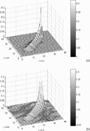
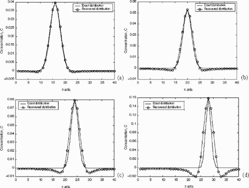
Applying our algorithm, and using only one conditioning point close to the maximum peak of concentration, we recover the spatial concentration distribution for those 8 different backward times. After normalizing the total time to 1, the recovered concentration corresponds to values of 20–90% back in time, starting from the initial (t = 0) backward time. Figure 1(b) presents all the recovered distributions so they can be compared to the exact distributions. These results are further plotted as transect profiles passing through the center of mass for each snapshot and in the x-direction, as shown in figure 2. It is worthwhile noting that the restoration is extremely accurate for up to 60% back in time. After that, even though the peak and mass errors are satisfied, the general shape is corrupted due to spurious undershoots and the corresponding overestimation of the high concentration values.

Figure 2. Exact and recovered concentration profiles at (a) 20%, (b) 40%, (c) 60%, and (d) 80% backwards in time.

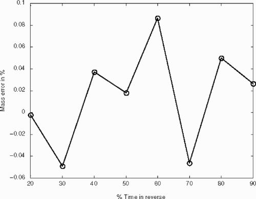
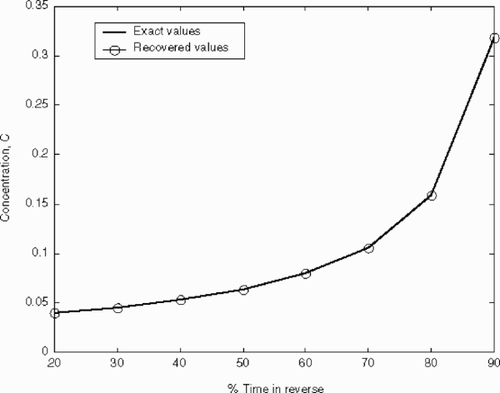
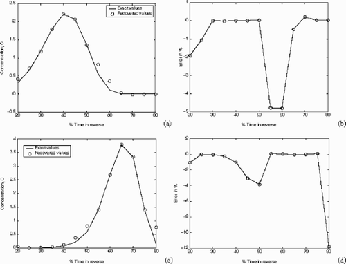
At each time snapshot, the performance of the restoration is also quantitatively evaluated by comparing the forward and the backward results and calculating the overall mass and relative errors at the observation or conditioning point(s). Figure 3 shows that the conservation of mass is satisfied and actually remains within ±0.2% no matter how far back in time we are trying to recover the plume history. Figure 4 shows the recovered concentration versus the exact values at the observation point as a function of backward time. This confirms that the error at this particular conditioning point remains within ±0.05% as required by the optimization program. Therefore, we assert that our algorithm is able to keep track of the increasing concentration of that moving observation or conditioning point as it optimizes for increasing backward times.

Figure 3. Evolution of the mass error.

Figure 4. Evolution of the concentration at the single mobile observation or conditioning point.

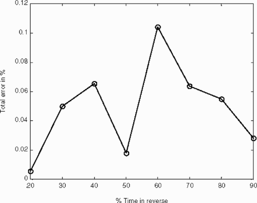
We also plot in figure 5 the evolution of the objective function, or total error, which again clearly shows that the procedure works well mathematically by satisfying the imposed constraints.

Figure 5. Evolution of the total error, which is a weighted sum of the mass error and the point concentration error.

5.2. Test case 2: five fixed observation or conditioning points

The second case entails a set of observation points that are fixed in space and is analogous to the plume being tracked by a network of bio- or chemical sensors that are stationary. In this case, the parameters of the problem are M = 100 kg, D_x = D_y = D = 0.6 km²/h and u = v = 2 m/s.

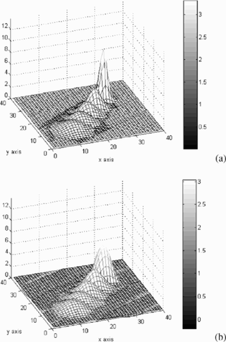
A forward simulation is conducted up to t = T_ft = 10 h. Figure 6(a) shows the evolution of the exact 2D distribution for 5 snapshots corresponding to forward time of 2, 4, 6, 9, and 10 h, the last one being to the forward terminal time at T_ft = 10 h. The concentration profile result at T_ft = 10 h is then assumed to be the present-day contamination distribution, which is the initial condition for the backward problem. Applying our algorithm, and using five conditioning points spaced uniformly along the a priori known path of the plume, we recover the spatial concentration distribution for various backward times. After normalizing the total time to 1, the recovered concentration corresponds to values of 20–90% back in time starting from the initial (t = 0) backward time. Figure 6(b) contains the recovered distribution obtained at the 20, 40, 60, and 85% backward times.

Figure 6. Evolution of the 2D plume profile (initial, 20, 40, 60 and 85% back in time). (a) Exact distribution and (b) recovered distribution.

A plan view of the plume can also be observed in the form of concentration contours in figure 7(a) (exact) and 7(b) (recovered) with the five observation or conditioning points identified as stars (*). The almost perfect correspondence of the exact and the recovered centroid of the plume is apparent.

Figure 7. Snapshots of 2D plume in the form of contours (initial, 20, 40, 60 and 85% back in time). (a) Exact distribution and (b) recovered distribution. Observation points are identified as stars (*) and concentration contours are shown only at the 1, 2, 3, 4, 4.5, 5, 5.5, and 6 levels.

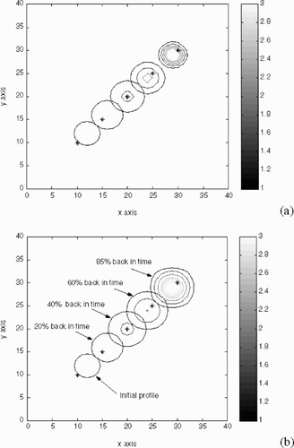
The simulation gave very good results up to a backward time of 65%, after which it became increasingly difficult to balance the error at the conditioning points with the mass balance error, as they become more and more “conflicting.” The location of the conditioning points relative to the plume is of critical importance, and it would be interesting to analyze how different network configurations can affect the accuracy of the reconstruction results in the future.

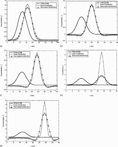
To emphasize this point, one can observe in figure 8, the performance of our reconstruction presented in the form of concentration transect profiles. Of particular interest are figures 8(c), (d), and (e). The reconstruction is considered to be excellent, very poor, and more than reasonably good for 60, 80 and 85% backward times, respectively. The poor performance of the reconstruction for 80% backward time is due to the location of the only two observation or conditioning points that are actively “sensing” the plume at this point in time (points 25, 25 and 30, 30). Because of these points’ location with respect to the plume, the method is incapable of improving the reconstruction as both mass balance and point errors are indeed minimal in this case. It is worth noting that this problem is quickly resolved for the 85% backward time as in this case the same observation points make a substantial difference due to their location relative to the plume.

Figure 8. Exact and recovered concentration profiles at (a) 20%, (b) 40%, (c) 60%, (d) 80%, and (e) 85% backwards in time.

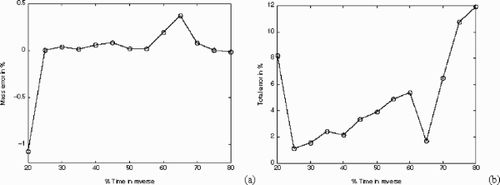
These observations are further supported by figures 9(a) and (b) depicting the behavior of the mass balance and the total errors as a function of time. Even though the mass balance error is generally less than 0.1% (with an occasional jump at 0.4%), the total error increases dramatically from ∼1–5% to 12% for the “problematic” 80% backward time case.

Figure 9. Time evolution of the (a) mass balance and (b) total error involved in the reconstruction.

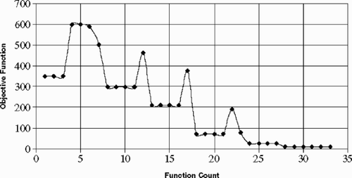
Consistent with these observations is the behavior of the optimization objective function, which is depicted as a function of the iteration count for a specific backward time in figure 10. As the contaminant plume relays information from each conditioning point, the optimization process must adjust in response to this new information and hence the objective function increases while new optimal parameters are identified and the process continues until the objective function minimum is attained.

Figure 10. Evolution of objective function for the reconstruction at 20% backward in time.

Finally, figure 11 presents the breakthrough curves, that is concentration versus time curves (10a and 10c) at the two most active of the five observation points (20, 20 and 25, 25) and the associated point concentration error (10b and 10d). Again, the performance of our method is deemed more than satisfactory with the reconstruction producing results that are both accurate (errors averaging less than 2–3%) and that also retain all the salient features of the measured or the observed breakthrough curves.

Figure 11. Breakthrough curve and corresponding evolution of the error at the conditioning point located at (a) and (b) (20, 20), and (c) and (d) (25, 25).

6. Discussion and conclusions

In this study, we have applied a mathematical method to solve a 2D homogeneous advection-dispersion transport problem backwards in time, and enhanced it by implementing an optimization scheme in order to facilitate and automate the reconstruction process.

The resulting Bagtzoglou-Baun method was then tested and analyzed for two different scenarios. In the first case, our method was capable of reconstructing the time history and location of a non-reactive plume that was released instantaneously. The reconstruction process was based only on a weighted average of the mass error and only one single moving monitoring sensor. That sensor was assumed to be moving along the centroid of the plume and at its known velocity. In the second test case, the objective function was again based on the mass balance error, but this time averaged with errors observed at five fixed monitoring sensors. These sensors were uniformly spaced along the a priori known path of the plume.

Several interesting observations can be drawn from our two test cases.

1.

In the first scenario, the time reconstruction of the 2D plume was successful at every time step, making it clear that even if only one sensor is available, as long as it is close to the centroid of the plume, the contamination source identification algorithm will perform very well.

2.

In the second scenario, the reconstruction is accurate only up to 65% backwards time. In general, the total error increases and the results become inconsistent as we go backwards in time. We believe that this is due to several factors. First, the position of the sensors relative to where the plume is moving is a critical parameter for a successful reconstruction. Second, the number of sensors is also an important parameter to be considered and there may be an ideal number of sensors to be used or activated during the optimization process.

Acknowledgments

ACB gratefully acknowledges the financial support of the University of Connecticut Research Foundation through grant FRS 445161 and the productive discussions with Professor David Miller of the University of Connecticut. SAB wishes to thank Daniel Cornacchiulo of Columbia University for his collaboration and support during the formative stages of this research effort. The authors acknowledge the constructive comments received by three anonymous reviewers and the editorial suggestions and efforts of the Associate Editor, Professor Helcio Orlande and the Editor, Professor George S. Dulikravich.

Additional information

Notes on contributors

Sandrine A. Baun †

Email: [email protected]

Notes

Email: [email protected]