Aerodynamic data modeling using support vector machines

Abstract

Aerodynamic data modeling plays an important role in aerospace and industrial fluid engineering. Support vector machines (SVMs), as a novel type of learning algorithms based on the statistical learning theory, can be used for regression problems and have been reported to perform well with promising results. The work presented here examines the feasibility of applying SVMs to the aerodynamic modeling field. Mainly, the empirical comparisons between the SVMs and the commonly used neural network technique are carried out through two practical data modeling cases – performance-prediction of a new prototype mixer for engine combustors, and calibration of a five-hole pressure probe. A CFD-based diffuser optimization design is also involved in the article, in which an SVM is used to construct a response surface and hereby to make the optimization perform on an easily computable surrogate space. The obtained simulation results in all the application cases demonstrate that SVMs are the potential options for the chosen modeling tasks.

Keywords:

• Aerodynamic data modeling
• Support vector machine
• Neural networks
• Application
• Mathematics Subject Classifications 2000: 76G25
• 76N15
• 68T05

1. Introduction

Many design and control problems encountered in flow machines and systems in aerospace and fluid mechanical engineering incorporate the aerodynamic data modeling. For example, an aircraft engine should be calibrated against its performance. A process gas-compressor, turbine or pump should be measured to obtain the performance curves, and a flow-field measurement tool or an instrument should be calibrated in static and dynamic conditions, etc. These aforementioned cases are just a few of the numerous examples in which aerodynamic data modeling may play an important role.

Aerodynamic data modeling can be viewed as a problem of the approximation of input-output function mapping from the available sample data that may be obtained through wind-tunnel experiments, or more recently, by numerical simulations. There have been many ways in which scientists and engineers can get an approximating analytic function from the aerodynamic data. The most-commonly-used approaches would be polynomial fits and spline functions [1–4]. However, the determination of the correct terms and coefficient range from the existing data for multivariate polynomial fitting or spline function is a difficult task. Neural networks (NNs), and, in particular, multi-layer feed-forward NNs, can be trained to approximate virtually any smooth, measurable nonlinear input-output relationships. In recent years, NNs have become popular in the aerodynamic data modeling field, and have produced promising results: NNs were successfully used as an estimator of jet engine performance [5]; NNs were applied in aerodynamic optimization design to construct a response surface for the design space to reduce the computing-time from the direct CFD analysis [6,7]; NNs were adopted for calibration of multi-hole aerodynamic pressure probes [8,9], etc. Nevertheless, some inherent drawbacks, such as slow training convergence speed, less than general performance, local minima and over-fitting problems, usually make NNs being restricted in their applications to practical problems. Hence, for aerodynamic data modeling, it is still worthwhile to go on to seek the approaches that are superior to the current approaches such as neural networks.

Support vector machines (SVMs), developed by Vapnik [10], are a novel type of statistical learning strategy. They are gaining popularity due to many attractive features and empirical performance [11–13]. SVMs embody the structural risk minimization (SRM) principle, which has been shown to be superior to the traditional empirical risk minimization (ERM) principle, employed by conventional neural networks. SRM minimizes an upper bound of the generalization error, as opposed to ERM that minimizes the error on the training data. It is this difference that equips SVMs with greater ability to generalize, and to achieve global minimum, which are just the goals in statistical learning. At the same time, SVMs can be theoretically analyzed and easily implemented. Real-world applications often mandate the use of more complex models and algorithms – such as NNs – that are much harder to analyze theoretically. SVMs can achieve both. They construct models that are complex enough: they contain a large class of neural networks, radial basis function (RBF) networks, and polynomial classifiers as special cases. Yet it is simple enough to be analyzed mathematically, because it can be shown to correspond to a linear method in a high-dimensional feature space nonlinearly related to input space. Moreover, even though a high-dimensional space is treated in an SVM, in practice, it does not involve any computations in this space. By the use of kernels, all the necessary computations are performed directly in the input space [13].

This article presents a pioneer and empirical study of using SVMs to model aerodynamic data. Mainly, the empirical comparisons are carried out with two practical modeling application cases to demonstrate how the SVMs perform over the commonly used NNs, which concern performance-prediction of a prototypic mixer designed for engine combustors, and calibration of a five-hole pressure probe. The work also includes a CFD-based diffuser optimization case, in which an SVM is used to construct a response surface for the design space so as to make the optimization able to perform on more easily computable surrogate space.

2. Overview of SVM regression

Originally, SVMs were developed for pattern recognition problems. Recently, they have been successfully extended to nonlinear regression estimation [14]. In regression formulation, the goal is to estimate an unknown continuous-valued function based on a finite number set of sample data (---261----1) (x_i is input vectors, d_i is the desired values). SVMs approximate the function by a linear regression (---261--1) in a feature space F. Here, (---261----2) , denote a set of nonlinear transformations from input space x to feature space F, and (---261----3) , b are coefficients.

Now the question is to determine (---261----4) , b from the sample data by minimization the regression risk, R_reg(f), based on the empirical risk, (---261--2) where C is a pre-specified constant determining the trade-off between the training error and the regression function flatness, L(d, f(x)) is a cost function that measures the empirical risk. The second term, 1/2∥w∥², is used as a measure of function complexity. In general, the ε-insensitive loss function is used as the cost function [11]. For this function, when the data points are in the range of ±ε, they do not contribute to the output error. The function is defined as (---261--3) SVM regression performs linear regression in the high-dimensional feature space using ε-insensitive loss function and, at the same time, tries to reduce model complexity by minimizing the term, 1/2∥w∥², in equation (2)(---261--2) . This can be described by introducing (non-negative) slack variables ζ, ζ* to measure the deviation of a sample outside the ε-insensitive zone. Thus SVM regression is formulated as the following minimization problem: (---261--4) (---261--5) Using the Lagrange function method to find the solution of the above problem can lead to a Quadratic Programming (QP) problem (---261--6) (---261--7) where α_i, (---261----5) are Lagrange multipliers introduced. K(x_i, x_j) is called kernel function. Its value is equal to the inner product of two vectors x_i and x_j in the feature space ϕ (x_i) and ϕ (x_j), i.e., K(x_i , x_j ) = ϕ(x_i) · ϕ (x_j). Any symmetric function satisfying Mercer's condition [10] can be used as the kernel function. The commonly used kernels include the linear kernel, the polynomial kernel, the Gaussian kernel and spline kernel [12].

Solving the above QP problem of equation (6)(---261--6) with constraints of equation (7)(---261--7) , the Lagrange multipliers α_i and (---261----6) can be determined. Therefore, the linear regression equation (1)(---261--1) becomes the following explicit form: (---261--8) So far, the regression to the data can be completed by the SVM method. Based on the nature of the corresponding QP, in general, only a number of coefficients α_i, (---261----7) will be assumed as non-zero, and the data points associated with the pair can be referred as “Support Vectors (SVs)” (from which SVMs get the name).

3. Empirical comparisons of SVMs and NNs with two practical modeling cases

3.1. Tasks and data

3.1.1. Performance-prediction of prototypic mixer

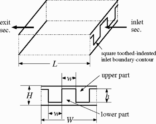
Recently, a novel prototypic mixer for flameless-oxidation engine combustors was investigated by one of the current authors [15]. In that work, a set of input–output data that sampled the mixing processes of the mixer was obtained through CFD numerical simulations. Here some of those data are taken for making up a modeling task for our application purposes. The mixer is simply taken as a “box”, as shown in figure 1, with the given height, length and width, denoted as H, L and W, respectively. The two cross-section-equal inlet channels, arranged up and down, are used to conduct the to-be-mixed cold air and hot air into the mixer chamber. The boundary-contour in the inlet section that separates the two inlet air streams is shaped as a periodic and square tooth-indent, which is determined in geometry with the height h and the width, w. A parameter, called Temperature Pattern Factor (TPF), is selected as a criterion to describe the mixer performance, which can be defined on the exit cross section of the mixer as (---261----8) , where T_max is the peak (or maximal) temperature at the section, and (---261----9) is the flow-weighted average temperature; the temperatures T₁, T₂ relate to the cold-air stream (upper) and the hot-air stream (lower), respectively. 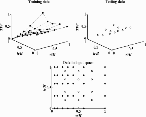Assuming that one's attention is focused on how the periodic inlet boundary-contour affects on the mixer performance, the modeling task can then be described as an approximation of the parameter, TPF, as a function of the two geometric parameters of the inlet boundary-contour, h and w, as (---261--9) The height and length of the mixer were kept constant as: H = 0.05 m and L = 0.2 m, while the width W can be determined in dependence on the cyclic status of the inlet boundary-contour. The temperatures of the cold air and the hot air are chosen as T₁ = 500 K and T₂ = 1000 K. The inlet cold air and hot air velocities are also kept in constant as V₁ = 150 m/s and V₂ = 50 m/s, respectively. The inlet geometric parameters h and w were selected within certain number of different values: h = 0, 0.015, 0.03, 0.04, 0.05 m, and w = 0.0025, 0.005, 0.01, 0.015, 0.02, 0.03, and 0.05 m. The commercial CFD code, STAR-CD, was used for the above experimental simulations. The high Reynolds number k-epsilon turbulence model, discretization strategies, such as UD scheme for convection terms and CD scheme for diffusive terms of governing equations, the well-known SIMPLE method for velocity-pressure linkage were applied in the numerical analyses [5]. From the above specifications and simulations, in total 35 experimental points were obtained. In addition, 12 testing points were also simulated that were prepared to assess the modeling. The training data points and testing data points are shown in figure 2.

Figure 1. Geometry and specifications of the prototypic mixer.

Figure 2. Training data and testing data for performance-prediction of the prototypic mixer.

3.1.2. Calibration of multi-hole pressure probe

Multi-hole probes are easiest-to-use and cost-effective devices for three-component velocity measurements of fluids in research as well as in industry environments. By measuring each pressure at the ports of a probe's tip and through the use of proper calibration methods, the multi-hole probes can measure the three velocity components, the total and static pressure of a flow-field at the location of its tip. Their calibrations are suitable for establishing the mapping relations between the pressure values measured in the multiple ports and the measured flow-field properties.

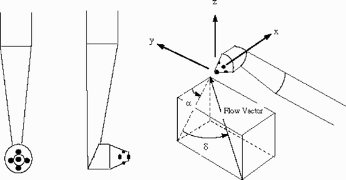
A five-hole probe with a conical tip is chosen in this example case. The configuration of the probe and its coordinate system is shown in figure 3. In the tip, one port sits at the center of the cone, while the other ports are axisymmetrically arranged in a ring downstream. Generally, a local velocity vector in the measured flow-field can be fully determined with four local flow parameters. They are the flow pitch angle, α, the flow yaw angle, δ, the total-pressure-coefficient A_t, and the static-pressure-coefficient A_s. Consequently, to calibrate the probe is to determine the above four variables (output variables) as functions of the five measured pressures or equivalently and more usually, two non-dimensional pressure coefficients, B_α, B_δ (input variables). Let P₅ denote the pressure measured at the central port, and P_i, i = 1, 2, 3, 4, denote the pressures at the other four ports. The pressure coefficients, B_α, and B_δ, are defined as: B_α = (P₅ − P₄)/P′, B_δ = (P₁ − P₃)/P′, where (---261----10) . From the calibration data, it can be found that both the total-pressure-coefficient, A_t, and the static-pressure-coefficient, A_s, have more non-linear relations with the measured port pressures compared with both flow angles, α and δ. For simplicity, in this application, only the output variables, A_t, and A_s, are considered. 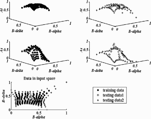The calibration of the probe is to establish the following function relationships (---261--10) The probe calibration data was obtained on an air jet calibration facility (i.e. a wind-tunnel). Varying the α and δ in steps of 5° from −30° to +30° respectively, the total 13 × 13 = 169 data points were obtained that form 169 input output pairs. From these data points, 101 are chosen as the training data that is used to establish SVMs, and two groups of testing data are prepared, namely, one with 20 points (Testing Data 1) and another with 48 points (Testing Data 2), for later-on different testing purposes. This data is shown in figure 4. Since the data is rather diverse in scales in this case, the values of each variable were normalized to [0, 1] in order to get more efficient training for SVMs and NNs.

Figure 3. Configuration of the five-hole pressure probe and its coordinate system.

Figure 4. Training data and testing data for calibration of the five-hole pressure probe.

3.2. Experimental results

Three SVMs were established, where one is for performance-prediction of the prototypic mixer and the other two for calibration of the total-pressure-coefficient and the static-pressure-coefficient of the chosen five-hole pressure probe. Meanwhile, the multi-layered feed-forward NNs are chosen as benchmarks for a comparison. Three NNs are constructed corresponding to the three established SVMs. Each SVM and its counterpart NN are trained with the same training data and tested with the same testing data. Mean square error (MSE) is used to measure the performance of training and testing processes for SVMs and NNs. The goal errors to be satisfied by the SVMs and NNs for training are chosen as: for performance-prediction of the prototypic mixer – 0.0005; for total-pressure-coefficient calibration – 0.00005, and for static-pressure-coefficient calibration – 0.0045.

3.2.1. Implementation of SVMs

The training work was performed with a Matlab toolbox for SVMs freely available in the Internet website http://www.isis.ecs.soton. ac.uk

In training the SVMs, some options need to be decided a priori. As examples of the kernel-scope methods the choice of kernel functions is of course, very important to SVMs. In addition, the performance of SVM training also depends on the two prescribed control parameters, C and ε. In general, the above options are problem-specific and can be determined through a trial-and-error process. In our cases, trial-and-error experiments for these options are done and the results show that when the three-order spline function is taken as the kernel function, and both C and ε as 100 and 0.001, respectively, the best possible results can be produced for any of our modeling tasks. Consequently, those options were selected in our application.

3.2.2. Founding of NN models

Each NN is specified as two-layered with a single-neuron-second layer to output the function parameters such as TPF, A_t and A_s, and is trained by the same data used to train the corresponding SVM. The number of the neurons in the first layer of each NN is determined through the trial-and-error processes to make it have an optimal topological structure for the selected modeling task and hereby to have a maximal competitiveness against the counterpart, the SVM. The following statistical procedure is implemented for each NN to find the optimal number of the neurons. Starting with a small neuron number in the layer, the NN is trained with the training data till a given goal error was satisfied. It was then used to predict the testing data, and the relating MSE was recorded. This training-predicting coupling operation was repeated for the chosen neuron number with 100 different initials of NN connection weights. The above steps were further repeated with progressively increasing neuron numbers from small to large. Average errors over the 100 runs under each given neuron number were used to evaluate the NN structures. From the experiments, the three NNs get their optimal neuron number in the first layer as follows. For performance prediction of the prototypic mixer, the NN is with 4 neurons in the first layer. For the calibration of the pressure probe, the NN for the total-pressure-coefficient is with 26 neurons in the first layer, while the NN for the static-pressure-coefficient is with 28 neurons in the layer. For all three NNs, the neurons in the first layer take the “tansig” transfer function, and the neuron in the second layer takes the simple linear transfer function. The BP algorithm is used for training. The training and the testing of all the NNs are implemented by using the NN toolbox in Matlab 6.1.

3.2.3. Results

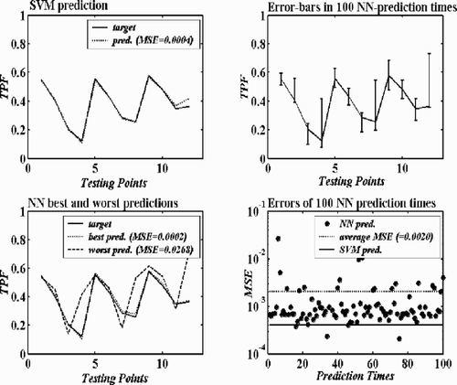
The SVM trained for performance-prediction of the prototypic mixer is examined in comparison with the corresponding NN through its testing data, while the two SVMs trained for calibration of the five-hole pressure probe – through the Testing Data 1 prepared for this case. For each case, the NN has 100 different prediction outcomes since it is trained with 100 different runs.

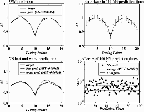
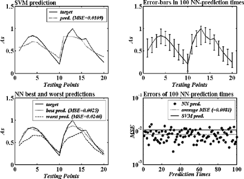
Some comparative results are obtained and shown in figures 5, 6 and 7. In each of these figures, the first subfigure presents the SVM prediction results to the related testing data, the second to the fourth subfigures present the NN prediction results to the same testing data. All the prediction errors are recorded and listed in the figures. From the results, the following facts can be found:

1.	For the case – performance-prediction of the prototypic mixer, the SVM performed quite better than the NN in predicting the testing points. The average error (0.0020) of 100 NN prediction times is much larger than the SVM prediction error (0.0004). Moreover, in 100 prediction times, only three times has NN been as accurate or better than the SVM prediction.
2.	For the case – calibration of the five-hole pressure probe, the results are more complicated. In the total-pressure-coefficient calibration, the SVM and the NN performed very similarly as they are in the case of the prototypic mixer. The SVM is better than the NN: the average error (0.00007) of 100 NN prediction times is larger than the SVM prediction error (0.00004), and in 100 prediction times NN has only 24 times been better or as good as the SVM prediction. On the other hand, in the static-pressure-coefficient calibration, the SVM cannot perform better than the NN. The SVM prediction error is 0.0109, a little bit larger than the average error (0.0081) of 100 NN prediction times. And in 100 prediction times, NN has 83 times been better than or as good as the SVM prediction.
3.	For all the selected modeling cases, the results from 100 NN different prediction times are quite random and varying with large ranges. This uncertainty phenomenon is of course unwelcome in any modeling, but it is an inherent drawback of NN-based modeling. To further explain this, it is needed to re-mention the principle of NN training. As is well known, NNs employ the ERM principle. So, training of an NN is to minimize an empirical risk function (in our cases, a mean square error function) that is multi-modal with many local minima. In the meantime, the training algorithms commonly used are gradient-based ones (e.g. BP algorithm in our cases), which easily fall into the local minima. As the results show, with different initials of the connection weights an NN training can attain different local minima and hereby get different results.

Figure 5. Testing results of the SVM and the NN in the case of performance-prediction of the prototypic mixer.

Figure 6. Testing results of the SVM and the NN in the case of calibration of the five-hole pressure probe – calibration.

Figure 7. Testing results of the SVM and the NN in the case of calibration of the five-hole pressure probe – the static-pressure-coefficient calibration.

3.3. An extended observation

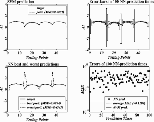
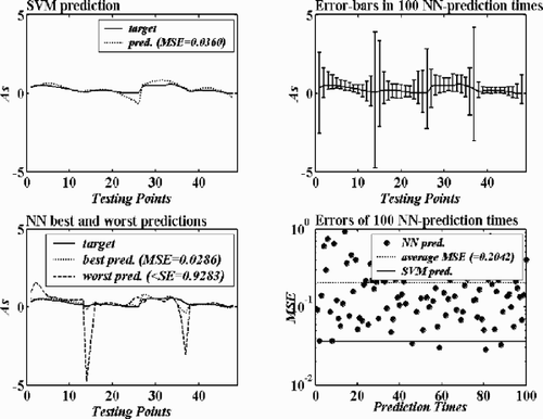
As aforementioned, with the learning principle SRM that differs from the ERM possessed by NN approaches, SVMs should have a better generalization ability than NNs. Our previous evaluations have been done only from the standpoint of interpolation, i.e., the predictions are made within the space spanned by the training data. In this sub-section an extended observation is performed to investigate the extrapolation ability – generalization ability – of the compared approaches. The case of calibration of the five-hole pressure probe is only chosen for this purpose. The two SVMs and two NNs established for both the total-pressure-coefficient and the static-pressure-coefficient are used to predict the Testing Data 2. These testing points are located outside the training data space (see figure 4). The prediction results are comparatively shown in figures 8 and 9, which prove the deduction on SVMs and NNs, that is, SVMs have a better generalization ability than NNs. In the total-pressure-coefficient calibration, the SVM predicts the testing points well with the prediction error as 0.0009, while all the 100 NN prediction results are worse than the SVM prediction (the NN best prediction error is 0.0054, the worst 0.4243, and the average 0.1184). In the static-pressure-coefficient calibration, the SVM does not perform as well as in the total-pressure-coefficient calibration, but is still quite acceptable. The SVM predicts the testing points with the prediction error as 0.0360, and NN predicted those points with errors as: the best 0.0286, the worst 0.9283 and the average 0.2042. In the 100 NN prediction times 4 are better than or as good as the SVM prediction. In addition, if comparing NN performance in these cases with that for interpolation, it can easily be found that the prediction ability of the NNs has become much worse with the recorded errors being much larger and more diverse. Furthermore, from the previous evaluations it is known that for interpolations the SVM is not superior to the NN in the case of static-pressure-coefficient calibration. However, for extrapolation problems with the same compared SVM and NN, the former proves to be better than the latter. This further indicates that the SVM has a good robustness feature in generalization performance.

Figure 8. Extended testing results of the SVM and the NN in the case of calibration of the five-hole pressure probe – the total-pressure-coefficient calibration.

Figure 9. Extended testing results of the SVM and the NN in the case of calibration of the five-hole pressure probe – the total-pressure-coefficient calibration.

4. Application in a diffuser design

In the CFD-based shape optimizations encountered in fluid and aerospace engineering, a fatal obstacle may be the time consumed to obtain the objective values. In general, during the optimizations, a certain number of candidate solutions are required to evaluate, especially, when the populated optimization methods, such as evolutionary algorithms, have to be applied to the problems. If a high fidelity CFD code, like a Navier–Stokes equations-based code, is employed into an optimizer to directly analyze each solution, the time taken by the optimization process may, in most of the cases, become too long to be acceptable. One commonly used measure taken to avoid this problem is to introduce the response surface technique into the optimization process. Response surface technique has an extensive application to many engineering optimizations. When the technique is used in the CFD-based shape optimizations, the response surfaces are usually taken as surrogates of the actual design space. The original design space is first sampled to get some experimental points deemed to well represent the original space through the chosen CFD code. The obtained data is then used to establish some response surfaces so as to make up the surrogates to the original design space, on which the optimization can be performed. Obviously, the establishment of the response surfaces is cast to the construction of a mapping relationship between a set of input-output data. As demonstrated earlier in this article, SVM will be a suitable candidate to such problems.

Diffusers are commonly used to convert dynamic pressure into static pressure rise. The problems of designing a diffuser for maximum pressure recovery or minimum total pressure loss has been found to be a well-suited touchstone for CFD-based optimization because of the relatively rapid and robust convergence conditions and the ease of interpreting optimum design solutions from underlying flow physics. Much work has been done in diffuser shape optimizations using the response surface technique. An interesting recent work was reported by Madsen et al. [16]. In this section, the SVM technique is applied to make up the response surface in a CFD-based diffuser optimization case. This simple example demonstrates the SVMs’ ability in this field.

4.1. Optimization problem

The diffuser to be optimized has an overall geometry as in [16]. The diffuser (figure 10) is two-dimensional, planar and symmetric, and defined by the ratio of the inlet and outlet areas AR and the length/height ratio L/D, where L is the axial length of the diffuser and D is its inlet throat half-width. The L/D ratio is fixed at 3 and the area ratio AR at 2.0. Expressed in terms of the inlet half-width D, the horizontal length of the inlet section is 1 D, whereas the horizontal length of the outlet is 10 D.

Figure 10. Two-dimensional, symmetric diffuser to be optimized.

The shape of the curved wall-section between the straight inlet and the outlet sections of the diffuser is to be optimally designed for a good performance of the diffuser. In order to make the search easier, this wall-section's contour is parameterized. There are many methods that can be used to perform the current parameterization. Because our current application is mainly illustrative, the contour is presented with a simple fourth-order polynomial function. Moreover, the contour in its two ends is asked to ensure C¹-continuity to connect to the straight wall-sections. The polynomial can then be determined with one control point, or its two coordinate parameters. For more simplicity, we specify the control point fixed horizontally at the central position of the curved wall-section. Accordingly, the contour of the curved wall-section is reduced being controlled with only a vertical coordinate parameter, that we denoted as y₁. To keep the contour to have an as high as possible monotonicity and the optimization to have an as large as possible search space, the appropriate value range of the parameter y₁ is defined as 0.9 ≤ y₁/D ≤ 2.1 through a cross-experiment.

The total pressure loss coefficient of the diffuser is taken as the objective to be minimized. It is defined by (---261----11) , where (---261----12) and (---261----13) are the inlet and outlet total pressures. The optimization problems can then become (---261--11)

4.2. Construction of response surface

Let the parameter y₁ varies in 25 different values uniformly distributed within the range 0.9 ≤ y₁/D ≤ 2.1. Consequently, 25 different wall-section contours are defined. For each contour, the corresponding flow-field is analyzed by the CFD method as described in the following and the function value, the total pressure loss coefficient is calculated.

The flow in our case is incompressible and fully turbulent with a Reynolds number Re_D = 4.28 × 10⁶, based on the inlet half-throat width. The two-dimensional unstructured flow analysis code [17] is applied which is based on the full Reynolds-averaged Navier–Stokes equations with the original k − ω two-equation turbulence model as a closure form. The computation domain is discretized using an unstructured mesh. The discretization of the governing equations is done using a finite volume method. Roe's flux-difference scheme has been used for inviscid fluxes. Directional derivatives along edges are used for viscous fluxes. The gradients at the mesh vertices are calculated using the Least-squares method.

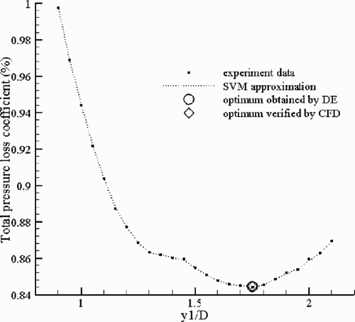
The obtained 25 input–output data pairs are then used to establish a SVM to be the response surface of the design space, i.e., to approximate the function relationship between the contour parameter y₁ to the total pressure loss coefficient (---261----14) . In the training of the SVM, the prescribed control parameters, C and ε are taken as 1000 and 0.001, by trial-and-error, and three-order spline function is taken as the kernel function. The samples points and the search space approximated by the SVM are shown in figure 11. From the figure, it can be found that the SVM well regressed the experimental data of the search space, so can be a good response surface approximating the space.

Figure 11. The experiment data, SVM approximation (response surface) to the search space and the DE optimum solution and its CFD verification in the diffuser optimization.

4.3. Optimization results and discussions

A promising novel evolutionary-algorithm-kind optimization method – differential evolution (DE) is applied to search the optimum contour of the diffuser. This method has been empirically demonstrated to be efficient, effective and robust [18]. As with any other evolutionary algorithm, DE works in a population of trial solutions, and through performing a set of different operations, including mutation, crossover and selection, among the individuals in the population to evolve the population to approach the optimal target. There are several variant versions of DE. The one called “DE/rand/1/bin-version”, which appears to be the most frequently used variant and is often considered as the “basic” version of DE [18], is chosen for our purpose.

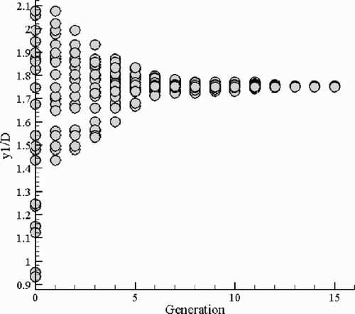
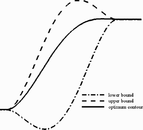
With the population size taken as 20, DE can search out the optimum contour in about 15 generations: from the divergent 20 trial solutions in initial population, DE quickly evolves the population, and at the 15th generation, the population almost converges to identical individuals (at the point y₁ = 1.7509), and attains the lowest position ((---261----15) ) in the response surface landscape. The searched optimum point is verified by the CFD code described earlier, and the experiment value of the total pressure loss coefficient for this point is 0.840%, almost identical with the value on the response surface (see figure 11). The above population evolving processes are recorded and shown in figure 12. Since our optimization problem is one-dimensional, it enables us to easily define the position where the optimum is and to conveniently evaluate the DE searched results. It can conclude that DE indeed finds the global optimum. The optimum contour is presented in figure 13, where the range of the search space is also shown. As we expected, the optimum contour should be with a good monotonicity that can ensure the flow goes “smoothly” through without a suddenly compressing-diffusing or diffusing compressing process to result in additional energy loss. Evidently, the contour located in the area near the bounds has a bad monotonicity, and thus has a bad performance.

Figure 12. The evolving process of the 20 trail solutions in a population in DE optimization.

Figure 13. The curved parameterized contour range and the optimum contour obtained by DE optimization.

It is also worthwhile to mention some time-consuming comparison here. In our current CFD experiment, the computation domain is discretized with about 4 × 10⁴ cells. It takes more than an hour to complete such an analysis in a general Unix system. If no response surface technique is taken into studied optimization, and if it is assumed that DE need the same generations to get the optimum solution, in our simplified diffuser case, about three hundred CFD analyses should be done, and consequently more than three hundred hours should be needed to complete the optimization. With the response surface technique introduced into the optimization, it is only needed to take time to get the experiment points to construct the surface (in our current case with 25 samples points only 25 CFD analyses are required). After the surface is set up, DE can complete the optimization in a very short time (e.g., several seconds to minutes). The fact that the response surface technique can make a CFD-based optimization to be able to solve in an acceptable time is proven with our simple case.

5. Conclusions

The application of the SVM approach in aerodynamic data modeling is studied and presented in this article. In principal, SVMs are empirically with the commonly used multi-layered feed-forward NNs as benchmarks in two practical modeling cases: (a) performance-prediction of a prototypic mixer that is designed for engine combustors; and (b) calibration of a five-hole pressure probe that is commonly used in 3-D flow-field measurements. From the experimental results it can be concluded that SVMs provide a promising alternative to fulfill the chosen modeling problems. For the performance-prediction problem, the established SVM performs evidently better than the NN. For the calibration problem, the SVMs perform better (in the case of the total-pressure-efficient calibration) or not better (in the case of the static-pressure-efficient calibration) than their counterparts. However, SVMs clearly demonstrate a good generalization ability, compared with the NNs in the selected observation case. The results also showed the very important superiority of SVMs over NNs – the high certainty. With different training, NNs can get different results. This inherent drawback of NNs is well eliminated in SVMs. The paper also involves a practical CFD-based diffuser optimization case in which SVMs can be applied. In the case that a SVM is used to construct a response surface to approximate the design space, in this way to avoid directly using a CFD code in the optimization process, thus to make the optimization to be solved in an acceptable time. Again, the simulation results demonstrate effective utilization of SVMs in this field.

Acknowledgements

Prof. Y. Levy from Aerospace Engineering Faculty, Technion, Israel, provided his kind permission to use the related simulation data, which is acknowledged with gratitude. The authors are also thankful to Ms. Victoria Hughes for editing the final version of this article.