Extension of the hot wire method to the characterization of stratified soils with multiple temperature analysis

Abstract

The aim of this article is to develop a practical device able to estimate a thermal conductivity profile in stratified media such as burned soils in Chile. The classical hot wire method consists of measuring the temperature response of a heat step imposed on a thin cylindrical probe by Joule effect. The main characteristic of the extension of the method consists of analyzing the two-dimensional temperature response of multiple thermocouples equally spaced along the heating cylinder. A semianalytical method (quadrupole method) is then implemented in order to obtain a transfer matrix between the heat flux excitation and the temperature response vectors. Such method is suitable to obtain asymptotic expansions in order to investigate the sensitivity analysis and the estimation strategy. A complete two-dimensional model is used in order to define a time window in which the one-dimensional radial heat transfer assumption is valid. Some experiments and estimation results are presented in a case where the characteristic diffusion times in the radial direction are small compared to the inter-layers diffusion time.

Keywords:

• Hot wire method
• Semianalytical method
• Sensitivity analysis

Introduction

Numerous works have been devoted to the thermal characterization of global properties of soils [1–5]. In the case of stratified media a local characterization versus the depth can avoid a tedious sampling of the different variety of soils.

The method proposed here is an extension of the classical hot wire method (see [6]). The principal interest of the hot wire method is: easiness to implement, rapidity of the data treatment and low cost. That is the reason why, in industry, this method of thermal characterization is well known and widely employed. This method was introduced at the beginning of the 30s, by Stalhane and Pyk [7] for the thermal conductivity measurement of granular materials. Now, due to the further evolution of this method, it is possible to characterize solids, liquids, gazes and porous medium [8–10].

The proposed extension of the method consists here in analyzing the temperature response of multiple thermocouples equally spaced along a heating cylinder. The resolution of the direct heat transfer problem is often difficult in such case because the heterogeneities are made of radial and stratified layers. A semianalytical extension of the quadrupole method [11] is implemented in order to find a transfer matrix between the heat flux excitation and the temperature response vectors. Such a method is convenient to obtain suitable asymptotic expansions in order to investigate the sensitivity analysis and the estimation strategy.

Experimental and estimation results will be presented, as an example, in the case where the characteristic diffusion times relative to the radial direction are small compared to the inter-layers diffusion time.

Position of the problem

The present study deals with the problem of finding a generalized intrinsic relationship between temperature and heat flux at the boundaries of a heterogeneous medium with one-dimensional varying properties versus layer direction. The extension of thermal quadrupole formalism is obtained from one-dimensional discretization versus z-direction, within a control volume formulation, coupled with the semianalytical solution of the corresponding vectorial differential equation – see [12] for more details.

In a medium with one-dimensional varying thermal properties, such as the one depicted in Fig. 1, without volumetric source term, the two-dimensional transient heat conduction is governed by the following equation: (---485--1-) with the boundary conditions (---485--1-) and the initial condition (---485--1-)

Figure 1 Two-dimensional conduction in an heterogeneous medium with one-dimensional varying thermal properties.

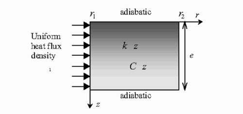
Here, the presentation of the two-dimensional direct model is developed by considering adiabatic conditions on lateral faces (z = 0 and z = e). Nevertheless, the same demonstration can be realized for broad boundary conditions; for more details see [12].

Space discretization of Eq. (1a)(---485--1-) is performed versus z-direction in order to estimate a profile of conductivity, k(z). As a rule of thumb, this technique can be applied to heterogeneous media in one direction (and particularly for stratified media). A number N of new variables is introduced as: (---485--2-) where i⁻ and i⁺ indicate the ith grid interfaces due to space discretization. Equation (1a)(---485--1-) is then integrated relative to z: (---485--2-) where ϕ is the heat flux density in the z direction. The heat flux density ϕ is linearized, and the interface thermal conductivities k_i− and k_i+ are introduced in the conservative form: (---485--2-)

Performing a Laplace transformation for i = 2 to N − 1, such as: (---485--3-) and substituting this expression into Eq. (2b)(---485--2-) yields: (---485--3-)

Both boundary conditions at z = 0 and z = e have to be expressed in the same way in order to obtain the corresponding equations at node i = 1 and i = N.

Introducing the vector (---485----1) of the N Laplace transformed temperatures at the position r, Eq. (3b)(---485--3-) can be written in the matrix form: (---485--4) with (---485---1) and (---485---2)

The operator “diag” is used in order to build a diagonal matrix from the corresponding vector. The square matrix (---485----2) on the left side of Eq. (4)(---485--4) is independent of r. Equation (4)(---485--4) can be solved directly by the diagonalization of this matrix. The diagonalization of this system yields: (---485--5-) where Ω is a diagonal matrix. Introducing the temperature vector in the new basis: (---485--5-) Equation (4)(---485--4) is then written as (---485--5-)

Each line of Eq. (5c)(---485--5-) can be solved directly in a scalar way, due to the fact that Ω is a diagonal matrix, and the corresponding equation is homogeneous. The general results can be arranged in a matrix form, applying the quadrupole formalism. Care must be taken in order to avoid the commutation of the matricial products: (---485--6-)

The general solution of Eq. (6a)(---485--6-) yields: (---485--6-) where I₀ and K₀ are the modified Bessel functions of zero order of the first and second kind, respectively. Coefficients d_k are function of the Laplace variable s, but are independent of r.

The scalar thermal quadrupole formalism is derived from the solution of Eq. (6a)(---485--6-) , by eliminating the integration constant G₁ and G₂ in Eq. (6b)(---485--6-) in order to find a linear relationship between temperature and heat flux in the Laplace space.

Introducing the flux expressed in the eigenvalues basis as j_k = −(2πr)Δz(dv_k/dr) or under vector notation: (---485--6-) The scalar thermal quadrupole at r₁ and r₂ location is written under the following form: (---485---3) or under vector notation: (---485--6-) where: (---485---4) and (---485---5) A_V, B_V, C_V and D_V are diagonal matrices. Subscript V refers to the fact that the temperature and heat flux vectors are written in the eigenvalues basis of matrix (---485----3) .

The boundary conditions in the r direction are given as a relationship between temperature and heat flux, but are unknown in the V basis. It is thus convenient to express J_V as a function of heat flux vector (---485----4) : (---485--7) where K is the diagonal matrix of thermal conductivity. Substituting Eq. (5b)(---485--5-) into Eq. (7)(---485--7) yields (---485--8)

Using Eqs. (5b)(---485--5-) and (8)(---485--8) , it is now possible to express the V-form quadrupole given by Eq. (6d)(---485--6-) as a generalized thermal quadrupole in terms of temperature and heat flux vectors in real space, such as: (---485--9-) or (---485--9-) with: A = PA_VP⁻¹; B = PB_V(KP)⁻¹; C = KPC_VP⁻¹; D = KPD_V(KP)⁻¹

When one of the boundary of the medium is located toward infinite in the r-direction, the corresponding coefficient G₁ in the scalar Eq. (6b)(---485--6-) has to be zero, in order to get a finite solution. Then, it is possible to find a direct relationship between Laplace temperature vector (---485----5) and Laplace heat flux vector (---485----6) at the position r₁, such as: (---485--10)

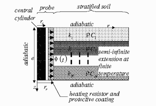
The main characteristics of the heat transfer problem are presented in Fig. 2. A central heating cylinder is inserted in the stratified medium. The response of several thermocouples equally spaced on the heating layer are recorded and analyzed after a heating step.

Figure 2 Schematic diagram of the heat transfer system and boundary conditions.

Then the complete system, described in Fig. 2, can be modeled as successive radial layers related to successive transfer matrices, such as:

a.	In the central cylinder (subscript: c), corresponding to the thermal properties of the stick (---485--11) The contact between the central cylinder and the protective coating is assumed as perfect.
b.	In the external cylinder (subscript: e) (made of the resin coating (subscript: r), the contact resistance between the probe and the semi-infinite soil (subscript ∞, Eq. (10)(---485--10) applied at the position rr) can be given by: (---485--12) with (---485----7)

It is then possible to express the interface temperature vector of the heating resistor versus the heating flux vector with the following expression (---485--13) where: (---485---6)

Such expression (13)(---485--13) is very similar to boundary element method, because it allows then to obtain a direct relationship between the boundary temperature and flux vector, instead of gridding a large domain. The numerical implementation of such expression is convenient with matrix solvers such as Matlab [13] and inverse Laplace transform such as Stehfest [14] (see also [11,12] for more details). However, due to the necessary diagonalization of the matrices at each time step, an iterative inversion method can be time consuming.

Asymptotic expansions

One other advantage of the semianalytical approach is to allow the implementation of asymptotic expansions.

1.	For short times (s → ∞)

The term “short times” should be considered as shorter than the inter-layer diffusion time such as (---485--14)

The matrix (---485----8) is then neglected in Eq. (4)(---485--4) which means that the heat transfer becomes one dimensional following the radial direction. The matrices A, B, C and D from Eqs. (9)(---485--9-) , (11)(---485--11) and (12)(---485--12) become diagonal and the relationship between the temperature and heat flux of each layer (i) is turned into: (---485--15) with: (---485---7) This result is equivalent, for each layer, to the classical one-dimensional case.

1.	Long times asymptotic expansion (s → 0)

A long time asymptotic expansion is now applied to Eq. (15)(---485--15) . Long times should be considered as (---485--16) Eq. (15)(---485--15) is then turned into (---485---8) Thus the double asymptotic expansion is only valid in a characteristic time domain, such as (---485--17) A necessary condition for this time domain to exist is (---485--18)

Also the probe inertia must be small enough in order to let the relative short times behavior to appear. Practically, analyzing the experimental temperature history versus the natural logarithm of time is the best way to ensure that the correct time domain is chosen. For example, in Fig. 6, we can notice the different zone (short times, valid time window and long times). Only for z = 0.07 and 0.09 m, the heat transfer becomes quickly two dimensional.

For the valid time window, a simplified expression of Eq. (15)(---485--15) is obtained (---485--19)

For the particular case of an input step heat flux, the classical hot wire method result applies such as (---485--20)

Before beginning the estimation of the thermal conductivity profile, it is necessary to have a good idea of the appropriate time window. In this domain, it is then possible to simplify, meaningfully, the transient two-dimensional problem in a succession of one dimension where the thermal conductivity can be identified by a simple linear regression.

The temperature evolutions calculated from expression (15)(---485--15) have been compared with a relative good agreement with the complete two-dimensional transient model given by Eq. (13)(---485--13) (with N = 50).

Sensitivity analysis

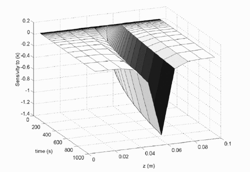
The sensitivity analysis is realized on a two-layers medium with ten temperature measurements (N = 10) (see Fig. 3). Both layers have the same thickness (e/2). The parameters of this problem are listed in Table I. Thanks to the two-dimensional transient model, the sensitivity of temperature vector T to the thermal conductivity k_i of each layer (i) can be studied (see Fig. 4 where i = 6) which permits us to confirm that T is mostly sensitive to the k_i = 6, and weakly to the adjacent layers, due to the sharp decrease of the sensibility coefficients around this layer. Moreover, the thermal conductivity and the specific heat are correlated (Figs. 4 and 5). The previous direct two-dimensional model is then used to find the correct time window where the one-dimensional transient model is valid. Therefore, in this time window, the estimation of the thermal conductivity profile can be realized with Eq. (20)(---485--20) .

Figure 3 Schematic diagram of the sensitivity analysis problem.

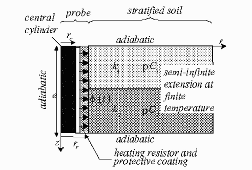
Table I Parameters of the sensitivity problem

Thermal properties	Heat flux	Geometry
k1 = 0.16 W m^−1 K^−1	ϕ = 0.3 W	e = 0.1 m
ρC1 = 1.46 MJ m^−3 K^−1		rc = 1.5 × 10^−3 m
k2 = 0.6 W m^−1 K^−1		rr = 2.1 × 10^−3 m
ρC2 = 4.18 MJ m^−3 K^−1
λc = 0.12 W m^−1 K^−1
ρCc = 1.25 MJ m^−3 K^1
λr = 0.2 W m^1 K^−1
ρCr = 1.6 MJ m^−3 K^−1

Figure 4 Sensitivity of temperatures T_i, i = 1, N to the thermal conductivity of layer i = 6.

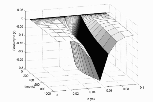
Figure 5 Sensitivity of temperatures T_i, i = 1, N to the specific heat of layer i = 6.

The aim of this article is to identify k for each layer corresponding to the number of temperature measurements. In order to verify and validate this method, we have tested a medium constituted with only two layers but eight temperature measurements. The two-dimensional model is used to find the good time window, regardless of the thermal conductivity profile.

The advantage of this probe is that it is easy to adapt in different conditions (thin layer, thick layer, type of medium). Moreover, it is cost effective.

Experiment

Experimental device

The experimental device is made of a wood stick as a central cylinder (of radius r_c = 1.5 × 10⁻³ m). The heating is realized with a metallic wire which is wound round the stick. The height thermocouples (K-type) were regularly spaced (Δz = 0.02 m) on the stick surface and are in contact with the heating wire. Such a device is coated with a protective polymer resin. The global length and the radius of the system are: l = 0.24 m and r_r = 2.1 × 10⁻³ m, respectively. The stick can be conveniently embedded in such stratified media as soils.

Test sample

In order to validate the methodology, a test sample was carried out with a two-layered medium. The first layer is a CMC-gel (CarboxylMéthylCellulosic), and the second one is a powder (semolina). The thermophysical properties of the media are measured separately and listed in Table II.

Table II Thermophysical properties of the media

Medium 1 (CMC-gel)	Medium 2 (semolina)
k = 593 mW m^−1 K^−1	k = 130 mW m^−1 K^−1
ρC = 4 × 10^6 J m^−3 K^−1	ρC = 1.05 × 10^6 J m^−3 K^−1

Results and discussion

The evolution of the experimental temperature responses is shown on Fig. 6. The power ϕ imposed on the heating wire is 2.08 W. The total experimentation time is about 600 s. The standard deviation of the temperature noise is 0.1 K.

Figure 6 Experimental temperature history vs. natural logarithm of time.

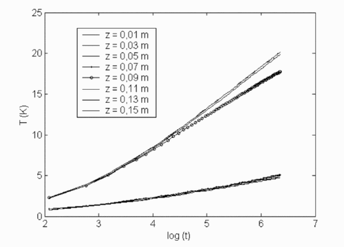
It can be observed that the temperature responses are uniform and corresponding to one-dimensional natural logarithmic evolution when the temperature sensors are far from the interface between the two materials. The two-dimensional transition (at z = 0.07 or 0.09 m) occurs only at long times as predicted by the asymptotic approximations.

From the previous observation, a simple least-square estimation based on one-dimensional radial transfer assumption (expression (20)(---485--20) ) is applied in order to estimate the thermal conductivity profiles. The result of such a very simple estimation process is reported in Fig. 7.

Figure 7 Thermal conductivity profile (real and estimated).

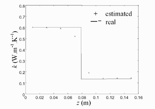
The relatively good agreement, shown in Fig. 7, justifies the application of such simple estimation method in this particular situation. It can be observed that the discrepancy due to two-dimensional effects is visible for the layers located near the interface (z = 0.08 m).

Conclusions

The main interest of this study is to present a technique suitable for the depth profile thermal conductivity retrieval, when both the thermal conductivity and specific heat properties are unknown. This ill-posed transient two-dimensional problem is split out into N convenient one-dimensional problems corresponding to the classical hot wire expansion technic.

A complete semianalytical two-dimensional transient model is implemented in order to define the convenient time domain where this simplification is useful.

Perspectives of this work are to investigate an estimation method related to the parameters based on the two-dimensional model. Such conditions as layers of small thickness compared to the stick radius can also be studied.

Nomenclature

Table

a	thermal diffusivity
A, B, C, D	generalized quadripole matrices
e	sample thickness
I0, I1	modified Bessel functions of first kind of order 0 and 1 respectively
K0, K1	modified Bessel functions of second kind of order 0 and 1 respectively
k	thermal conductivity
l	length of probe
N	number of mesh
P, P^−1	eigenvectors matrix
rc	radius of central cylinder
rr	global radius of probe
R	contact resistance
R	contact resistance matrix
s	laplace variable
t	time
T	temperature
ρC	specific heat
(---485----9)	laplace temperature
(---485----10)	laplace temperature vector
Δz	distance between nodes
ϕ	heat flux in the r direction
ϕ	heat flux density in the z direction
(---485----11)	laplace heat flux
(---485----12)	laplace heat flux vector
Ω	diagonal eigenvalues matrix

Acknowledgments

This work was partially funded by the FONDECYT program (Award # 1020349) as well as the DICYT Dept. Of the Universidad de Santiago. The authors gratefully acknowledge this support.

Additional information

Notes on contributors

R. Santander

E-mail: [email protected]

Notes

E-mail: [email protected]