Use of a single heated surface for the estimation of thermal conductivity components of orthotropic 3D solids

Abstract

This article deals with the experimental design and with the solution of an inverse parameter estimation problem, for the identification of the three thermal conductivity components of an orthotropic solid. The experimental setup examined here involves the heating of a specimen in the form of a parallelepiped, through part of one of its surfaces. Different experimental variables are chosen by using the D-optimum criterion, including the number and location of sensors and the size of the heating surface. The unknown parameters are estimated with the Levenberg-Marquardt method of minimization of the least-squares norm.

Keywords:

• Inverse parameter estimation
• Levenberg-Marquardt method
• D-optimum criterion

Introduction

Due to the importance of nonisotropic materials in nowadays engineering, such as composites, a lot of attention has been devoted in the recent past for the identification of their thermal properties through inverse analysis techniques of parameter estimation [1–13].

The choice of various optimal experimental variables, including the number and locations of sensors, as well as the heating and final times, for the model used by Sawaf and Özisik [1] for the estimation of thermal conductivity components of orthotropic solids, was addressed by Mejias et al. [8]. In these two works [1,8], the solid was considered in the form of a cube, with three of its surfaces heated by fluxes of equal magnitude, while the other three surfaces were assumed as insulated. Later, Mejias et al. [10,11] have examined in the experimental design the choice of the boundary conditions for the nonheated surfaces of the cube, as well as the choice of the magnitudes of the applied heat fluxes and of the body dimensions. It was found [10] that the use of constant temperature boundary conditions, instead of insulated boundary conditions, could result in more accurate estimates for the unknown parameters. It was also found [11] that the body dimensions and the magnitudes of the applied heat fluxes should be chosen in accordance with a transformation that maps the orthotropic solid into an isotropic solid [14]. In this case, the three thermal conductivity components could be estimated with identical relative accuracies. Despite such an important feature for the experimental design, the implementation of the experimental setup devised was not simple, because it involved the uniform heating of three surfaces of the solid and the magnitudes of the applied heat fluxes needed to be known for the inverse analysis.

In order to overcome such difficulties, we examine in this article an alternative experimental setup for the estimation of the three thermal conductivity components of orthotropic solids. In such a setup, only one of the surfaces of the solid would be partially heated. It would consist of a heater placed between two identical specimens of the material with unknown thermal conductivity components, thus allowing for better control of the magnitude of the applied heat flux, as well as of its distribution. We note that two-dimensional versions of this setup were examined in references [3,12,13]. The D-optimum criterion [15–18] is used here for the experimental design, involving the choice of different variables, like the number and location of sensors and the size of the heating surface. The Levenberg-Marquardt Method of minimization of the least-squares norm [15,19–21] is applied as the estimation procedure by using simulated measurements with random errors, as described below.

Direct problem

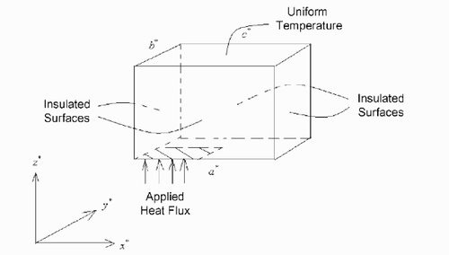
The physical problem considered in this work consists of a parallelepiped with dimensions a*, b* and c*, in the x*, y* and z* directions, respectively, as depicted in Fig. 1. The solid is initially at the uniform temperature (---501----1) . For times t* > 0, the boundary at z* = 0 is partially heated though the surface defined by 0<x* < (---501----2) and 0<y* < (---501----3) , while the remaining surface of this boundary is supposed to be insulated. The boundary at z* = c* is kept at a constant and uniform temperature (---501----4) and the other four boundaries are insulated. The solid is assumed to be orthotropic, with thermal conductivity components (---501----5) and (---501----6) in the x*, y* and z* directions, respectively, and the physical properties are assumed constant. The mathematical formulation of such physical problem is given in dimensionless form as (---501--1-) (---501--1--) (---501--1--) (---501--1-) (---501--1-) (---501--1-) The heat flux supplied at the surface z = 0 is given by (---501--2) where (---501--3) In Eq. (3)(---501--3) , t_h is the dimensionless heating time.

Figure 1 Geometry and coordinates.

The following dimensionless variables were defined in order to write the physical problem in dimensionless form: (---501--4--) (---501--4--) (---501--4--) (---501--4--)

In Eqs. (4a–o)(---501--4--) , (---501----7) and l* are characteristic values for thermal conductivity, heat flux and length, respectively. The superscript “*” appearing above denotes dimensional quantities, while ρ and c_p are the density and specific heat of the body, respectively.

In the direct problem associated with the physical problem described above, the three thermal conductivity components k_x, k_y and k_z, as well as the solid geometry, initial and boundary conditions, are known. The objective of the direct problem is to determine the transient temperature field T(x, y, z, t) in the body. The solution of the direct problem was obtained analytically by using the Classical Integral Transform Technique, with a domain transformation that maps the heat conduction equation for the orthotropic medium into the equation for an isotropic medium [14]. The analytical solutions for the heating and nonheating periods are given respectively by

• Heating Period (0 < t≤ t_h): (---501--5-)

• Nonheating Period (t > t_h): (---501--5-) where (---501--6--) (---501--6--) and the eigenvalues are given by: (---501--7--)

Inverse problem

For the inverse problem considered here, the thermal conductivity components k_x, k_y and k_z are regarded as unknown, while the other quantities appearing in the formulation of the direct problem described above are assumed to be known with a high degree of accuracy.

For the estimation of the vector of unknown parameters P^T = [k_x, k_y, k_z], we assume available the transient readings of M temperature sensors. The temperature measurements may contain random errors. Such errors are assumed to be additive, uncorrelated and normally distributed, with zero mean and a known constant standard-deviation σ. Also, for the estimation procedure we consider that no previous information regarding the parameter values is available. Therefore, the solution of the present parameter estimation problem can be obtained through the minimization of the ordinary least-squares norm, which is a minimum variance estimator in this case [15]. The ordinary least-squares norm is given by (---501--8) where (---501--9-) and each element (---501----8) is a row vector of length equal to the number of sensors M, that is, (---501--9-)

We note that Y_im and T_im(P) are the measured and estimated temperatures, respectively, for time t_i, i = 1, … , I, and for the sensor m, m = 1, … , M. The estimated temperatures are obtained from the solution of the direct problem by using the current available estimate for the vector of unknown parameters P^T = [k_x, k_y, k_z].

For the minimization of the least-squares norm (5)(---501--5-) , we apply the Levenberg-Marquardt method [15,19–21]. The iterative procedure of such a method is given by: (---501--10) where μ^k is a positive scalar named as damping parameter and Ω^k is a diagonal matrix.

The sensitivity matrix, J^k, is defined by [15] (---501--11-) where (---501--11-)

The purpose of the matrix term μ^kΩ^k in Eq. (10)(---501--10) is to damp oscillations and instabilities due to the ill-conditioned character of the problem, by making its components large as compared to those of J^TJ, if necessary [15]. The damping parameter is made large in the beginning of the iterations. With such an approach, the matrix J^TJ is not required to be nonsingular in the beginning of iterations and the Levenberg-Marquardt method tends to the Steepest Descent Method, that is, a very small step is taken in the negative gradient direction. The parameter μ^k is then gradually reduced as the iteration procedure advances to the solution of the parameter estimation problem and then the Levenberg-Marquardt method tends to the Gauss Method [15]. However, if the errors inherent to the measured data are amplified, generating instabilities on the solution as a result of the ill-conditioned character of the problem, the damping parameter is automatically increased. Such an automatic control of the damping parameter makes the Levenberg-Marquardt method a quite robust and stable estimation procedure, so that it does not require the use of the Discrepancy Principle in the stopping criterion to become stable, like the conjugate gradient method [21].

Statistical analysis

By performing a statistical analysis it is possible to assess the accuracy of (---501----9) , j = 1, 2 and 3, which are the values estimated for the unknown parameters P_j, j = 1, 2 and 3. By taking into account the statistical hypotheses described above, the covariance matrix for the ordinary least-squares estimator is given by [15]: (---501--12) where J is the sensitivity matrix and σ is the standard deviation of the measurement errors, which is assumed to be constant. We note that Eq. (12)(---501--12) is exact for linear estimation problems and is approximately used for nonlinear parameter estimation problems.

The standard deviations for the estimated parameters can thus be obtained from the diagonal elements of V as (---501--13) where V_jj is the jth element in the diagonal of V.

Confidence intervals at the 99% confidence level for the estimated parameters can be obtained as [15]: (---501--14) while the joint confidence region for the estimated parameters is given by [15]: (---501--15) where (---501----10) is the value of the chi-square distribution with 3 degrees of freedom for a given probability.

Design of optimum experiments

Optimum experiments can be designed by minimizing the hypervolume of the confidence region of the estimated parameters, in order to ensure minimum variance for the estimates. The minimization of the confidence region given by Eq. (15)(---501--15) can be obtained by maximizing the determinant of V⁻¹, in the so-called D-optimum design [15–18]. Since the covariance matrix V is given by Eq. (12)(---501--12) , we can then design optimum experiments by maximizing the determinant of the Fisher's Information Matrix, J^TJ [15–18]. Therefore, optimal experimental variables are chosen based on the criterion. (---501--16)

For cases involving a single sensor, each element F_r,s, r, s = 1, 2 and 3, of the matrix F ≡ J^TJ is given by: (---501--17) where I is the number of measurements.

If we take into account constraints, such as a large but fixed number of transient measurements of M sensors and also the maximum temperature in the region, T_max, we can choose to maximize the determinant of a normalized form of F, here denoted as F_I [15], the elements of which are given by: (---501--18) where t_f is the duration of the experiment.

Results and discussions

For the results presented below we assume the solid with unknown thermal conductivity components in the form of a cube, so that the characteristic length used to obtain the dimensionless problem is taken as l* = a* = b* = c*. Also, the characteristic heat flux is taken as (---501----11) , so that q₀ = 1 in Eq. (3)(---501--3) .

We note that for nonlinear estimation problems, such as the one under scrutiny in this work, the analyses of the sensitivity coefficients and of the determinant of F_I are not global, because these quantities are functions of the unknown parameters. Therefore, a priori estimated values for the parameters are required for the design of optimum experiments. For the test-cases examined in this article, we used the following dimensionless values for the thermal conductivity components in order to design the experiment: k_x = 1, k_y = 15 and k_z = 15. Such values were chosen based on the work of Dowding et al. [5] for the estimation of the thermal conductivity components of two-dimensional carbon–carbon composites. The dimensionless thermal conductivity k_x = 1 implies that (---501----12) . For the design of optimum experiments, involving the maximization of the determinant of (J^TJ), we took into account the constraints of a large and fixed number of measurements for each sensor, as well as the maximum temperature in the region, so that the matrix F_I with elements given by Eq. (18)(---501--18) was used in the analysis.

Design of optimum experiments

Before proceeding to the analysis of the transient variation of the determinant of the information matrix, let us examine the transient variation of the normalized sensitivity coefficients for different sensor positions. The sensor positions examined in this work are presented in Table I. They include sensors located at the center of the lateral thermally insulated surfaces at y = 1 (sensor 1) and x = 1 (sensor 2), as well as sensors located on the surface in contact with the heater at z = 0 (sensors 3, 4 and 5).

Table I Sensor locations

Sensor	Sensor location
1	(0.5, 1, 0.5)
2	(1, 0.5, 0.5)
3	(0.25, 0.25, 0)
4	(0.5, 0.5, 0)
5	(0.75, 0.75, 0)

The normalized sensitivity coefficients were obtained by multiplying the original sensitivity coefficients by the parameters that they are referred to. The normalized sensitivity coefficients with respect to the parameters k_x, k_y and k_z are defined respectively as (---501--19--)

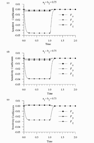
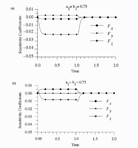
Figure 2(a–e) presents the normalized sensitivity coefficients for sensors 1–5, respectively, by assuming the size of the heating surface as a₁ = b₁ = 0.75. The heating time was supposed to be t_h = 1. Figure 2(a–e) shows a strong tendency toward linear dependence of the sensitivity coefficients for all sensor positions. Therefore, it is not possible to estimate the three unknown parameters with the readings of a single sensor. On the other hand, it may be possible to estimate the parameters with the readings of more than one sensor, because the constants of proportionality between the sensitivity coefficients are not the same, at the different sensor positions. Note in Fig. 2(a–e) that the sensitivity coefficients tend to zero after the heating is stopped at t = 1. However, before becoming zero, the sensitivity coefficient with respect to k_z undergoes a small increase for sensor 2, as depicted in Fig. 2(b). It can be noticed in Fig. 2(a–e) that, generally, the sensitivity coefficient with respect to k_z has the largest magnitude among the sensitivity coefficients, for any sensor position. The magnitude of F_z is larger for sensors 3, 4 and 5, located at z = 0. However, note in Fig. 2(c–e) that the magnitude of F_z decreases when the sensor is located towards the edge of the heating surface. The sensitivity coefficient F_z is negative for sensors 3, 4 and 5, because an increase in the thermal conductivity component k_z tends to decrease the temperature over the heating surface. Figure 2(c–e) also show that the sensitivity coefficients with respect to k_x and k_y are negative for sensors 3 and 4, but positive for sensor 5. Such is the case because an increase in the thermal conductivity components in the x and y directions tends to decrease the temperature of sensors 3 and 4 located over the heating surface, but tends to increase the temperature of sensor 5 located at the edge of the heating surface. The largest magnitude of F_x takes place for sensor 2, located at the surface x = 1. Similarly, the largest magnitude of F_y takes place for sensor 1, located at the surface y = 1, although the magnitude of F_y for sensor 3 is practically the same as for sensor 1.

Figure 2 Normalized sensitivity coefficients for: (a) sensor 1; (b) sensor 2; (c) sensor 3; (d) sensor 4; (e) sensor 5.

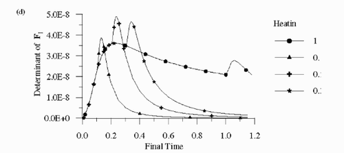
Figure 3(a–d) presents the transient variation of the determinant of the information matrix for different heating times, by assuming available the measurements of four different sensor configurations, which are presented in Table II. Configuration 1 consists of the sensors located at the insulated surfaces, sensor 1 at y = 1 and sensor 2 at x = 1, which have the largest magnitudes for F_y and F_x, respectively. Configurations 2–4 were composed by sensors 1, 2 and of one of the sensors located at the boundary z = 0, i.e., sensor 3 for configuration 2, sensor 4 for configuration 3 and sensor 5 for configuration 4. Sensors 3, 4 and 5 have the largest magnitudes for F_z. The results shown in Fig. 3(a–d) were obtained for a₁ = b₁ = 0.75.

Figure 3 Determinant of the information matrix for the: (a) sensor configuration 1; (b) sensor configuration 2; (c) sensor configuration 3; (d) sensor configuration 4.

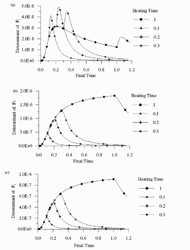
Table II Configurations for the sensors

Configuration	Sensors
1	1 and 2
2	1, 2 and 3
3	1, 2 and 4
4	1, 2 and 5

Figure 3(a) shows that the determinant of the information matrix undergoes a sudden increase at the moment when the heating is stopped, for configuration 1. This is a result of the change of the shape of the sensitivity coefficient with respect to k_z for sensor 2 when the heating is stopped, which undergoes a small increase before tending to zero (see Fig. 2b). For configuration 1, the optimum heating and final times are 0.2 and 0.24, respectively, when the determinant of the information matrix is maximum.

A comparison of Fig. 3(a–d) shows that the magnitude of the determinant of the information matrix increases when a sensor at z = 0 is used in the analysis, in addition to sensors 1 and 2, with the exception for configuration 4 (see Fig. 3d). The configuration with the maximum determinant of the information matrix is configuration 2, because sensor 3 has the largest magnitude for the sensitivity coefficient with respect to k_z (see Fig. 2c–e). As the sensitivity coefficient with respect to k_z decreases, when the sensor at z = 0 is moved towards the edge of heating surface, the maximum determinant of the information matrix decreases and, for configuration 4, the effects of the use of measurements of a sensor at z = 0 are negligible. We note in Fig. 3(b,c) that, for configurations 2 and 3, the determinant of the information matrix decreases at the moment when the heating is stopped. Such is the case because the sensitivity coefficients tend to zero very fast when the heating is stopped, with the exception of F_z for sensor 2, as depicted in Fig. 2(a–e). Therefore, for these configurations the effect of the sudden decrease in the sensitivity coefficients when the heating is stopped is more significant than the change in the shape of F_z for sensor 2. As a result, the heating time shall be chosen identical to the final time for configurations 2 and 3.

Configuration 2 is the best among those examined because of the maximum value obtained for the determinant of the information matrix. Hence, more accurate estimates are expected with configuration 2 than with the other configurations. For the results presented below obtained with such configuration we have used t = t_h = 1 because the determinant of the information matrix is practically constant for larger times.

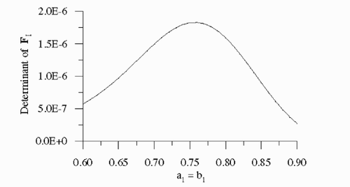
Let us now examine the effects of the size of the heating surface on the maximum determinant of the information matrix. Figure 4 shows the maximum values of such determinant, obtained with configuration 2 for t_f = t_h = 1 and for different sizes of the heating surface. Figure 4 shows that the optimum size of the heating surface is a₁ = b₁ = 0.75. For smaller sizes of such surface, the sensitivity coefficients decrease in magnitude and become more linearly-dependent, resulting in a decrease of the value of the determinant of the information matrix. For larger sizes of the heating surface the physical problem tends toward a one-dimensional problem, independent of the thermal conductivity components in the x and y directions, also resulting in a decrease of the values of the determinant of the information matrix. We note that the best sensor configuration was not changed for the different sizes of the heating surface.

Figure 4 Effects of the size of the heating surface on the determinant of the information matrix for t_f = t_h = 1 and sensor configuration 2.

In order to address the sample orientation effects on the design of the experiment, we also examined an alternative arrangement of the thermal conductivity components along the three principal axes involving k_x = 15, k_y = 15 and k_z = 1, instead of k_x = 1, k_y = 15 and k_z = 15 as examined above. For such arrangement, the best configuration consisted of three sensors located at (1, 0.5, 0.5), (0.25, 0.25, 0) and (0.75, 0.75, 0), with a₁ = b₁ = 0.4 and t_f = t_h = 0.05. However, the maximum determinant of the information matrix was about 10⁻¹⁰ for this alternative arrangement because of smaller magnitudes of the sensitivity coefficients.

Parameter estimation with simulated measurements

We now examine the estimation of the three thermal conductivity components of orthotropic solids, by using the Levenberg-Marquardt method of minimization of the least-squares norm. Table III summarizes the different test-cases examined, as well as the results obtained for the estimated parameters and for the 99% confidence-interval widths. In Table III, test-cases 1–3 correspond to the thermal conductivity arrangement 1, that is, k_x = 1, k_y = 15 and k_z = 15, while test-case 4 correspond to arrangement 2, that is, k_x = 15, k_y = 15 and k_z = 1. Test-cases 1–3 involve different initial-guesses for the unknown parameters for arrangement 1: for test-case 1, the initial guess was P⁰ = [0.5, 0.5, 0.5], for test-case 2 the initial guess was P⁰ = [1, 1, 1] and for test-case 3 the initial guess was P⁰ = [10, 10, 10]. For test-case 4 involving arrangement 2 the initial-guess was P⁰ = [0.5, 0.5, 0.5]. The results presented in Table III were obtained with 100 transient simulated measurements per sensor, of three sensors arranged in accordance with the best configuration specified in the section above. The duration of the experiment and the heating time were also specified in accordance with experimental design performed above, that is, for test-cases 1–3 we used t_f = t_h = 1 and for test-case 4 we used t_f = t_h = 0.05. The results presented in Table III were obtained with measurements containing random errors with standard-deviation σ = 0.01Y_max (where Y_max is the maximum measured temperature). In order to avoid biased results because of the random number generator used to compute the simulated measurements, the estimated parameters and the 99% confidence intervals presented in Table III were averaged over 50 runs of the inverse problem solver, obtained with different sets of simulated measurements.

Table III Test-cases and estimated parameters

Test-case	Arrangement	kx		ky		Kz
		Estimated value	99% Confidence interval width	Estimated value	99% Confidence interval width	Estimated value	99% Confidence interval width
1	1	1.00	0.02	14.96	0.55	15.01	0.05
2	1	1.00	0.02	15.04	0.55	15.00	0.05
3	1	1.00	0.02	15.07	0.55	15.00	0.05
4	2	16.35	7.40	14.35	6.27	1.00	0.01

An analysis of the results obtained for test-cases 1–3, involving different initial-guesses for arrangement 1, shows that the estimation procedure is not sensitive to the initial-guesses used here. Also, the results for these test-cases show that more accurate estimates are obtained for k_z than for k_y. This is caused by the larger sensitivity coefficients with respect to k_z than with respect to k_y for this arrangement (k_x = 1, k_y = 15 and k_z = 15), as illustrated by Fig. 2(a–e). The 99% joint rectangular confidence region, obtained by the multiplication of the 99% confidence interval widths of the three parameters, for arrangement 1 (test-cases 1–3) is 0.0006. The 99% joint rectangular confidence region for arrangement 2 (test-case 4) is 0.46. The larger confidence region for arrangement 2 is a result of the smaller determinant of the information matrix when compared to arrangement 1, as discussed above.

Conclusions

In this work we examined the estimation of the three thermal conductivity components of an orthotropic solid, by using one single heated surface. The D-optimum criterion was used for the design of the experiment. The optimum size of the heating surface, as well as the heating and final times, was obtained for different sensor configurations and for two different thermal conductivity arrangements. The inverse problem of parameter estimation was solved with the Levenberg-Marquardt method of minimization of the least-squares norm. The confidence regions of the estimated parameters were significantly reduced through the proper design of the experiment, so that accurate results were obtained by using in the inverse analysis simulated transient measurements containing random errors.

Nomenclature

Table

a, b, c	body dimensions along the x, y and z directions, respectively
FI	information matrix
I	number of measurements per sensor
Fx, Fy, Fz	normalized sensitivity coefficients for the thermal conductivity components along the x, y and z directions, respectively
J	sensitivity matrix
kx, ky, kz	thermal conductivity components along the x, y and z directions, respectively
M	number of sensors
P	vector of unknown parameters
S(P)	ordinary least-squares norm
th	heating time
tf	duration of the experiment
T	vector of estimated temperatures
Y	vector of measured temperatures

Greeks

Table

σ	standard-deviation of the measurements
σj	standard-deviation estimated for parameter Pj

Superscripts

Table

*	dimensional variables
k	number of iterations

Subscripts

Table

i	refers to time ti
m	refers to sensor M

Acknowledgments

This work was partially funded by the CNPq grant 522.469/94-9 and by the FAPERJ grant E-26/170.344/2000.

Additional information

Notes on contributors

M.M. Mejias ‡

E-mail: [email protected]

E-mail: [email protected]

Notes

E-mail: [email protected]

E-mail: [email protected]

E-mail: [email protected]