Transient and steady state free convection from a horizontal cylinder

Abstract

Estimating parameters in steady state, homogeneous systems is a well-developed process, usually involving the least squares technique or the Bayesian statistical approach. When the parameters vary with time or space, the process is more difficult. The function specification method was developed to estimate time varying surface fluxes for inverse heat conduction problems. Electrical and systems engineers tend to utilize the Kalman filter approach in such situations. The two approaches have much in common and the Kalman filter can often be applied to conduction/convection problems. It is particularly useful when multiple parameters vary with time. In addition, it lends itself conveniently to situations in which the measured data are noisy and/or correlated. This article describes the application of both methods to the problem of transient and steady state free convection from a horizontal cylinder. The problem involves noisy data and an exceptionally strong early time variation of the heat transfer coefficient. Because of the inherent smoothing effect of the Kalman filter, it is possible to estimate the heat flux with greater precision. The article discusses both approaches and compares the resulting estimates of the parameters.

Keywords:

• Horizontal cylinder
• Free convection
• Bayesian statistical approach

Introduction

The prediction of parameters in a model of a real process by an inverse technique is not complete unless some estimate of the precision of the estimated parameter can be provided. For parameters which are constants, this is usually obtained through the classical least squares approach. For time varying parameters the precision is usually assessed by comparing the simulated response to the measured response. Unfortunately, frequently one may find that a good agreement between the responses does not imply an acceptable level of precision in the estimated parameter. In addition, most tests of inverse techniques are based upon a simulated noisy response obtained by adding noise to the predicted response under the assumption that the noise is stationary and white. In reality, the measured response often contains nonstationary and colored noise. These effects may be eliminated when estimating constant parameters, but they can cause serious difficulty when treating time or spatially varying parameters. This article compares the use of the function specification approach [1,2] with the extended Kalman filter method [3,4] in the estimation of the transient convective heat transfer coefficient for free convection from a horizontal cylinder.

The experiment

Consider the transient convection from a horizontal cylinder which has a substantial thermal capacitance and whose surface flux thus varies significantly with time. The experiment takes place in a setting with varying air temperature, local drafts, and a strong radiation component. At steady state the heat transfer will be a function of the Rayleigh number (which is proportional to T_s − T_a) and the surface emissivity. In addition to estimating the steady state behavior, we are interested in how well such correlations predict the time varying convective flux when the cylinder is heating. Experiments were performed at different heating levels to produce a range of steady state surface temperatures, and thus Rayleigh numbers, to investigate the validity of the steady state correlations reported in the literature [5,6] and to determine if they were applicable to transient heating.

The experiment consisted of measuring the temperature history of a hollow copper cylinder, 33.5 mm OD, 9.33 mm ID, and 33.6 cm long. Twelve thermocouples were staked 0.2 mm below the surface around and along the cylinder and an electrical heater inserted into the center. The cylinder was suspended in room air and surrounded by a wire mesh enclosure, located 30 cm horizontally away from the cylinder to dampen any air flow perturbations. Local air temperature was measured at a point 6 cm horizontally from the cylinder axis. The cylinder surface was covered with a very thin dense layer of soot so that it radiated as a black surface. After the cylinder was determined to be in equilibrium with the ambient air, a constant heater power was applied and the power and temperatures were measured with a data acquisition system at 5 s intervals. A statistical analysis of the measurements gave the ranges and standard deviations (σ) shown in Table I.

Table I Experimental conditions

Measurement	Range	σ
Heat flux Q/A	2100 W/m^2	3 W/m^2
Ts	295–417 K	0.1 K
Ts − Ta	2–120 K	0.2 K

Comparison of measured and modeled responses

Because a conjugate cfd simulation of the system using FIDAP [7] showed that the temperature in the cylinder was isothermal to within 0.1 C, the cylinder was modeled as a lumped parameter transient conduction problem with a time varying convective heat transfer coefficient. Figure 1 compares the measured temperature and surface flux histories for a typical case.

Figure 1 (a) Temperature history; (b) Heat flux history.

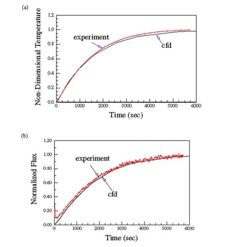
While the figures suggest that there is good agreement between the measured and the predicted temperatures, a closer examination reveals that there are important differences, particularly at early times. These effects are better illustrated by comparing the values of the convective heat transfer coefficient, given in terms of the Nusselt number Nu = hD/k, where (---535--1) as predicted by the function specification method using a value of r = 5 with the cfd predictions as shown in Fig. 2. The function specification method (Eq. (4) of Ref. [1]) is based upon minimizing the mean squared error given by (---535--2) where T_{n + j − 1} is the temperature measured at time (n + j − 1)Δt and Y_{n + j − 1}(h) is the predicted temperature based upon values of h(n + j − 1), and r is the tunable parameter.

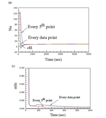
Figure 2 Nusselt Numbers estimated by the function specification method with r = 5 and from the cfd simulation.

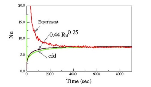
We note that the steady state values are in good agreement, but the transient values differ substantially at early times. The good agreement of the cfd results with those obtained from the correlation Nu = 0.44 Ra^0.25 using the measured temperatures suggests that the flow was able to adapt within seconds to the heating and that the correlation would adequately predict the transient behavior except at times less than a few seconds. The question is then what is the cause of the different behavior of the values obtained from the inverse solution and whether these differences reflect a basic fault in the model of the process.

White and colored noise

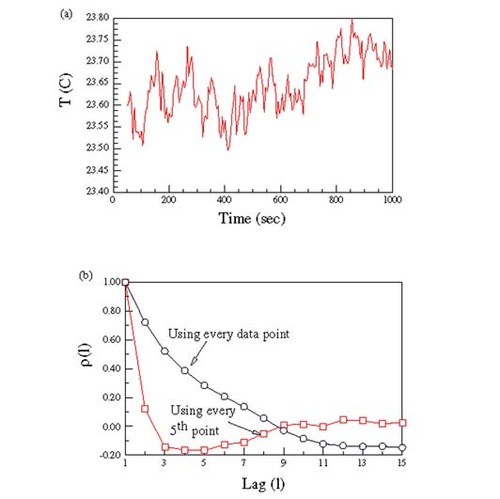
Before describing the inverse model in detail, it is important to realize that in almost all studies of the inverse method the noise is assumed to be stationary and white. That is, the mean and standard deviation of the noise are constant with time and the errors are statistically independent. Rarely do the the studies examine the consequences of violating these assumptions. Although the measurements of heater power and temperature were noisy, the most important and dominant noise was in the measured ambient temperature. Figure 3(a) shows a characteristic history. A spectral analysis [8,9] of this history showed that the noise was stationary, but decidedly not white. The effect that this “coloration” of the noise has on the estimated precision is quite dramatic. We can appreciate this effect by considering how the precision of the heat transfer coefficient at steady state is related to the noise in the measured temperatures. Since h is defined by (---535--3) the precision of the average value (---535----1) is given by the law for propagation of errors [10] by (---535--4)

Figure 3 (a) Typical time history of the ambient temperature; (b) autocorrelation coefficient for the ambient temperature shown in Fig. 3(a).

where we have assumed that the errors in Q, T_s, and T_a are independent. Now using the usual least squares approach to determine the mean value of T_a we have (---535--5-) (---535--5-) where One is a vector of N ones, One^T is its transpose, and W is the covariance matrix of the noise. If the noise is white and stationary, W is a diagonal matrix with diagonal elements having the constant value of (---535----2) and the standard deviation of the average ambient temperature is given by the usual expression [11] (---535--6) However, if the noise is colored, then W is a full matrix and the degrading effect of coloration is a significant increase in (---535----3) from that which would be computed by assuming that the noise is white, i.e. W is diagonal. Figure 3(b) shows autocorrelation coefficient ρ(l) defined as (---535--7) of the ambient temperature shown in Fig. 3(a) for different values of the lag, l. Values of ρ less than 0.2 in absolute magnitude are usually taken to mean that there is minimal autocorrelation [12]. From the figure, it is apparent that a significant autocorrelation, i.e., coloring, exists. An analysis of the information content shows that it is equivalent to that contained in white noise sampled at 1/5th the rate. The lower curve in Fig. 3(b) shows the effect of this lower sampling rate. Table II gives the respective values of the standard deviations of (---535----4) computed using the full matrix W (i.e. correlated noise) and that computed by assuming that the errors were uncorrelated (a diagonal W).

Table II Standard deviation of the average T_a

Sampling rate	Full W	Diagonal W	Ratio
Every date point	0.1266	0.0567	2.23
Every 5th point	0.0520	0.0513	1.01

Assuming that the noise is white substantially underestimates (---535----5) when every data point is used because of the high degree of correlation. On the other hand, when a reduced sampling rate is used, the noise is essentially uncorrelated. The consequence of ignoring the effects of correlation is that σ(h_ss) would be underestimated by over a factor of 2 as illustrated by Table II.

As described in the following section, the least squares solution for h requires a knowledge of W. Because it adds significantly to the computational costs of the least squares method and because it is neither easy nor convenient to evaluate [3,4], every effort should be made to ensure that the errors are not correlated. Fortunately, reducing the sampling rate is often an effective way to eliminate the correlation as shown above. Of course, this then means that rapidly varying parameters may not be well estimated.

Steady state results

The history of Nu shown in Fig. 2 was determined with the function specification method which is designed to estimate time varying parameters. Instead of choosing h(t_i) to match the measured response at time t_i to the model solution, the value of h(t_i is chosen to minimize the variance of the error in (---535----6) found by a least squares solution using the responses measured at (---535----7) .

Although the points used are usually at future times, r_b = 0, r_f > 1, one could just as easily use a combination of forward and backward points. r is an adjustable parameter and its optimal value often varies throughout the entire history of h(t) but it is generally more convenient to use a constant value [1]. Since the noise is assumed to be stationary and white, the procedure can be applied without a knowledge of σ(noise), and in fact the solution is independent of the noise which only enters into the final estimate of the standard deviation of the estimated parameter. The method is a form of data smoothing. The steady state values of Nu were best fit with Nu = 0.44 Ra^0.25 which differs from the published correlation by ≈10% and from the correlation of Chu and Churchill [6] by less than 5%.

Figure 4 compares the standard deviations of h_ss as a function of the number of points, r, sampled in the forward variable approach using Eq. (8)(---535--8) . (---535--8) where the summation was taken over the values h(t_i) during the period of steady state. Although the function specification method was designed for varying parameters, it proves to be effective when there is noise and, in our case, when the ambient temperature is constantly changing throughout the experiment. Increasing r reduces the uncertainty, but of course increases the computational cost.

Figure 4 σ(h_ss) as a function of the function specification parameter r.

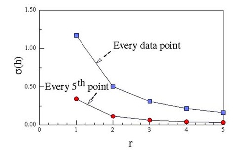
The reduction in σ(h_ss) is dramatic. The method as originally proposed assumes that the noise is white, i.e., all points are equally weighted, which we know from Fig. 3(b) is not the case. Using every 5th point, as suggested by Fig. 3(b), gives the results shown by the lower curve in Fig. 4 and the significant improvement in the precision of the estimate is clearly seen. Not only is the uncertainty in h_ss reduced, but the computational cost is much less. Note that the reduction in σ(h_ss) is in line with the results given in Table II.

Transient results

Using either the values of h derived from the cfd simulation or assuming a constant value over a short time, it can be shown that the sensitivity, ∂T/∂h, is zero at time zero and slowly increases to a maximum at steady state. Because of the very small sensitivity at short times, the experiment is not suitable for estimating h(t) at the start of heating. However, by 100 s, the sensitivity has increased to 0.1 C/(W C/m²) which with the value of σ(T_s − T_a) of 0.2 C gives a value of σ (Nu) ≈ 2, and increasingly smaller values as time increases. The imprecision is of the order of the oscillations shown in the time history of h in Fig. 2, giving a range of h not much different than that shown in the figure. This being so, one would conclude that the experimentally determined values of h are statistically different from the cfd simulation results. The obvious question is why? A possible approach to answering this is through the Kalman filter method in which the history of σ(h) is tracked and in which multiple parameters or other possible effects are easily incorporated. The idea behind the Kalman filter is to estimate a value of the parameter at time t_i based upon all of the data up to and including that at time t_j. If j < i the process is termed prediction, if j = i filtering, and if j > i smoothing. In essence the function specification method is really the Kalman smoothing filter approach in which the covariance matrix is assumed to be diagonal with constant elements and the past data are downgraded in importance.

Consider the determination of a constant parameter using the least squares approach with N data points. Usually, the data is treated in a batch mode, i.e., all N data points are considered at once. Assuming that the temperature can be expressed as a function of the convective coefficient, h, as (---535--9) (---535--10-) (---535--10-) where A is a N-dimensional vector with components of (---535----8) is the vector of measured temperatures and W is the covariance matrix of the noise. While the solution of Eq. (10)(---535--10-) gives the estimate of h and of σ(h) based on all N data points, the solution involves substantial computational expense when N is large and it is not easy to monitor how the error behaves as new data points are added. The recursive least squares approach was designed to allow a new datum point to be considered without inverting the entire matrix. It also permits one to monitor the behavior of σ(h) as N increases.

The Kalman filter is an extension of the usual recursive least squares approach based upon state variables which has been found in its usual formulation to handle slowing varying parameters. Details are given in a number of excellent texts [3,4]. The time history is presumed to follow the model (---535--11) where [S] represents an error in the thermal storage and [L] an unmeasured heat loss from the cylinder (see text following Fig. 5). The state of the system at time t_i is defined by the m component vector, y_i. In this study, (---535----9) where T_i is the temperature and h_i is the convective heat transfer coefficient at time t_i. y_i is given in terms of y_i − 1 by the equation (---535--12-) where dT / dt is determined from Eq. (11)(---535--11) , f_i is a forcing function (in this case the heater power) and w_i is the process noise with a covariance matrix of Q_i. The measured response, z_i, is given by (---535--12-) where n_i is the measurement noise which has a covariance of R_i. Both noises are assumed to be white i.e., Q and R are diagonal matrices, and to be uncorrelated with each other. Let (---535----10) represent our estimate of the system state at time i based upon measurements up to time i − 1. The procedure consists of the following steps

1.	a prediction of the response (---535----11) based upon (---535----12) . (---535--13-)
2.	and a correction (---535--13-)

The gain matrix, G_i is chosen to minimize the mean square errors of the state variables and is recursively computed from (---535--14) where P_i|i is the conditional covariance matrix of the error in the estimated state variable (---535--15) whose diagonal elements are σ²(T) and σ²(h). Figure 5 illustrates the histories of σ(T) and σ(h) corresponding to the Nu shown in Fig. 2. Both the estimated temperatures and the heat transfer coefficients show acceptably low standard deviations. Based upon these results, one would conclude that the estimated history of Nu was correct. However, this estimated history is at variance with the cfd simulations and requires an explanation.

Figure 5 Time history of: (a) σ(T); (b) σ(h).

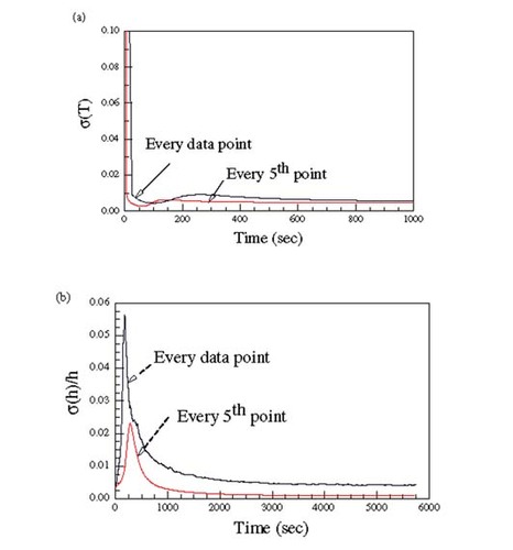
The most probable cause of the differences in h is an inadequacy in the model to represent the early time behavior. Even if the early time value of h were of the order of 10 times the steady state, the Biot number would still be of the order of 0.01, validating the use of the lumped capacitance model to estimate h. Since the value of h(t) is directly proportional to the surface flux which is the difference between the heat supplied to the cylinder by the heater, Q, and that stored in the cylinder, an error in estimating either quantity would give erroneous values of h.

One of the convenient features of the Kalman filter approach is the ease with with additional state variables can be included. In our case, an augmented state variable, (---535----13) , where L_i represents the unknown heat loss from the insulated ends of the cylinder and S_i represents an error in the heat stored because of the finite capacitance of the heater which is not represented by the measured cylinder temperature. Figure 6 compares the estimated surface heat flux based upon the original solution and that including either L or S. We note how much better the fluxes agree when a loss variable is included, suggesting that the heat supplied to the cylinder was in error especially at early times.

Figure 6 Estimated surface heat flux showing the effect of considering heat losses, L and errors in the energy stored, S.

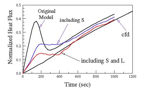
Since there is a contact resistance between the heater and the cylinder, it is possible that at early times the measured heater power does not represent the heat into the cylinder. Instead, the heater may be significantly hotter than the cylinder, thus storing heat in itself and losing heat out through the ends.

Both effects had been anticipated and hopefully mitigated by insulating the ends of the cylinder and using a thermal grease at the interface between the heater and cylinder. Thermal grease usually contains metallic particles (often copper) and is of very high viscosity, thus making it difficult to insert the heater when copiously used. A new cylinder was constructed and sufficient grease applied that a hydraulic press was required to insert the heater. In addition, thermocouples were installed at the heater/cylinder interface to more accurately characterize the temperature associated with the stored energy.

Figure 7 depicts the estimated heat flux and the time history of σ(h) for the new system. The experimental results are now in much better agreement with the cfd simulation, compare with Fig. 2, except at very early times. Comparable results were found using the function specification method. As expected, the standard deviations are reduced when the sampling rate is reduced, but of course doing so reduces the ability to represent the early transient effects.

Figure 7 (a) History of h for the new system computed using the Kalman filter; (b) history σ(h) for the new system computed using the Kalman filter.

Could better results be obtained at the earlier times to validate the cfd simulations? Theoretically yes, but realistically no. At very early times the sensitivity to h is small and the noise in the difference, T_s − T_a, is large compared to the difference, leading to very high values of σ(h). Furthermore, to get values of h at times in the range of 10 s would require a very high sampling rate, leading to a high degree of correlation and a further increase in the uncertainty.

The Kalman filter can account for colored noise, but only with a high-computational cost for analyzing the noise and including it in such a way that the filtering estimator yields a stable computation.

Furthermore, unless a strong fading memory is used, this approach reflects the total past history leading to a transient response which would be too slow for this specific problem. In addition, one would be required to very accurately measure the time history of the heater power and to eliminate, or at least to accurately determine, the heat losses associated with the momentarily high heater temperatures.

Conclusions

The use of the Kalman filter made it possible to track the history of the uncertainties and to determine the times when the heat transfer coefficient was most poorly estimated. By then expanding the state variables to include losses and imprecision in the estimate of the stored energy we were able to recognize that the difficulty was most probably due to interfacial resistance. When the resistance was reduced, substantially better results were obtained.

The Kalman filter approach is not a total panacea for problems like this. While it allows for the inclusion of fading memory, variations in how the terms in the alogrithm, Eq. (9)(---535--9) , are evaluated, and including varying degrees of smoothing, the method is very much ad hoc in nature. Since all of these are choices made by the analyst, usually based upon a subjective interpretation of the results, there are no well-defined procedures or criteria for making them.

In analyzing the results and predicting the history of h, both the forward variable and Kalman filter approaches estimated the temperature history of the cylinder very well as evidenced by the very small values of σT, being in the order of 0.05 C. Looking at the time history of σ(T) and σ(h), one would conclude that the inverse estimation of h was accurate unless a reason to suspect the results was known. In this case, the results of the cfd simulation and the correlation makes it clear that the inverse estimation of the first experiment, and even that of the second at early times, are significantly in error. This once again reinforces the idea that one must know much about the problem and must design the experiment carefully before conducting it.

Nomenclature

Table

A	surface area
B	matrix
D	cylinder outside diameter
E ( )	expected value
h	convective heat transfer coefficient
(---535----14)	mean value of h
hss	steady state h
k	thermal conductivity of the air
J	least squares function
l	lag
L	heat loss
Nu	Nusselt number (hD/k)
Q	heat supplied by heater
r	function specification method parameters
Ra	Rayleigh number
S	error in heat stored
t	time
Δt	sampling time
Ta	ambient temperature
Ts	surface temperature
x	column vector
x^T	transpose of x
y	state variable vector
(---535----15)	estimated value of y
(---535----16)	conditional expectation
σ()	standard deviation
W	covariance matrix of noise
∑	covariance matrix of the errors in the state variables

Acknowledgment

This work was conducted under the sponsorship of the Sandia National Laboratories, Albuquerque, NM. The author wishes to acknowledge the support of the laboratory and the helpful assistance of Drs. S. Kempka, B. Blackwell and K. Dowding.