The logistic regression model is a member of a general class of models called log-linear models. These models are particularly useful when studying contingency tables (tables of counts). Such tables occur when observations are cross-classified using several categorical variables (contingency tables are sometimes called cross-classifications). The logistic regression form is then appropriate if one of the categorical variables takes on two values and can be viewed as a target variable. For example, in clinical trials, whether the patient lives or dies is a reasonable target variable, and different variables could be potential predictors (for example, gender, membership in the treatment or control group, presence or absence of certain symptoms, etc.).
The following is an examination of an unusual mortality episode. The dataset consists of 2201 observations, corresponding to all of the people originally exposed to the mortality agent. For each of the people, there are recorded four variables:
STATUS: Economic status
1 = High status
2 = Medium status
3 = Low status
4 = Other
AGE: Age
0 = Child
1 = Adult
GENDER: Gender
0 = Female
1 = Male
SURVIVED: Survival of person
0 = Did not survive
1 = Survived
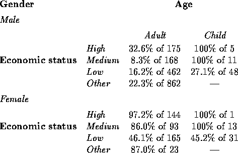
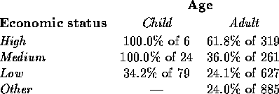
Here is a summary table of these data, given as survival percentages of the number of people of that subgroup at risk (each subgroup is termed a covariate pattern):
Note that there were no children in the “Other” economic status class.
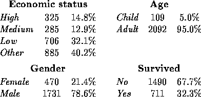
A first look at the data can be through the use of frequency distributions, since all of the variables are categorical (these take the place of histograms). Percentages are given as a percentage of the 2201 people at risk.
We see that almost all of the people at risk were adults, more than three-fourths were men, and about two-thirds did not survive. The unspecified “Other” economic status class is noteworthy, as it alone accounts for more than 40% of the people at risk.
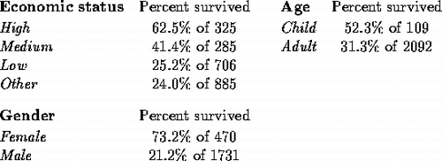
Two-dimensional contingency tables correspond to scatter plots in continuous data regression modeling. They cannot tell us how the predictors work together to model the probability of survival, but they can give indications of what is going on marginally. Since the survival variable is the response of interest here, the tables are given in terms of survival percentages for people of that class.
The chance of survival is apparently related to all three of these factors. Mortality was much higher for men than for women, and higher for adults than for children. The observed survival percentage is directly related to economic status, with higher status associated with higher survival probability (“Other status” has lowest survival percentage, but of course that does not guarantee that it corresponds to lowest economic status).
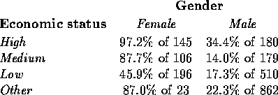
Three-dimensional contingency tables allow us to assess the possibility of interaction effects among the predictors. These can be presented as two-way tables, with survival percentages given in each cell. Recall that an interaction effect represents an association not accounted for by the main effects. First, the interaction of economic status and gender:
The most striking pattern here is the difference between “Low status” and the others. While for the other three status levels mortality was much higher among men than among women, for “Low status” the difference is much smaller, with less than half of the women surviving (that is, low economic status female survival percentage is considerably lower than would be expected from the main effects alone).
The following table summarizes the interaction of economic status and age:
This interaction also makes clear the different nature of “Low status” compared with the others; while no children of the other classes died, almost two-thirds of those in “Low status” did.
Finally, the following table represents the interaction of age and gender:
Adult women had a higher survival rate than girl children did, but for men the survival rate was twice as high for children than for adults.
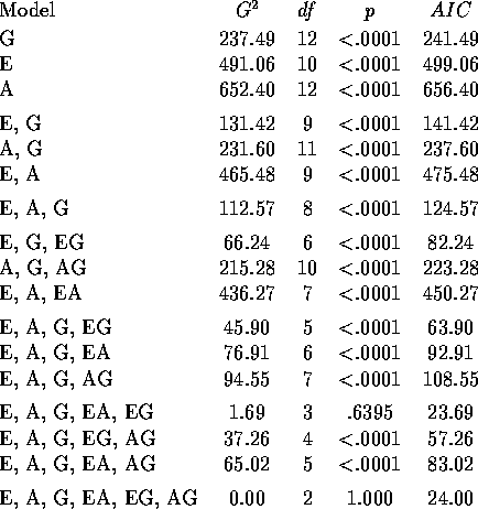
We can use logistic regression to try to decide which of these potential effects are useful to build a model predicting survival probability accurately. The following table summarizes the properties of the models considered. All of the models are hierarchical, in that the presence of an interaction effect in the model implies that the associated main effects are also present. Since there were no children with “Other” economic status, the interaction between economic status and age (EA) is fit using only two of the effect codings corresponding to pairwise products of those for the main effects, rather than three (the groups that take the value −1 for each effect coding are “Other status” and “Child,” respectively). The likelihood ratio goodness-of-fit statistic () is given for each model, along with associated degrees of freedom (df) and tail probability (p). The Akaike Information Criterion (AIC), is given in the last column (it equals
). The models are given ordered from smallest to largest AIC value within model class (one main effect, two main effects, three main effects, etc.) to make model selection easier.
According to , the only two models that fit the table include the two interactions EA and EG, or all three pairwise interactions EA, EG and AG. We must recognize, however, that the large sample size means that statistically significant effects might not have great practical importance. Similarly, while the three models with minimum AIC include all of the main effects and two or three interaction effects, the well-known tendency of AIC to lead to overfitted models (as we discussed in the context of least squares regression modeling), implies that more care in choosing a model that fits adequately but is parsimonious is called for.
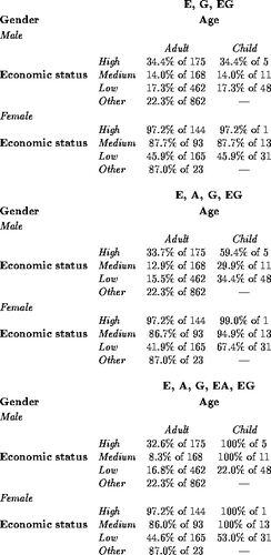
One way of doing this is to compare the fitted values for the three models [(E, G, EG), (E, A, G, EG), and (E, A, G, EA, EG)] that were the best-fitting models of their respective classes. These are given below.
The fitted survival percentages are very similar for all three models for the adult classes, but differ for the child classes. Since children represent less than 5% of the total population at risk, the simple model (E, G, EG) seems adequate to describe the important associations with survival in the data. Here is a summary of the results of fitting this model:
Logistic Regression Table Odds 95% CI Predictor Coef StDev Z P Ratio Lower Upper Constant 1.8971 0.6191 3.06 0.002 STATUS High 1.6653 0.8003 2.08 0.037 5.29 1.10 25.38 Medium 0.0705 0.6863 0.10 0.918 1.07 0.28 4.12 Low −2.0607 0.6355 −3.24 0.001 0.13 0.04 0.44 GENDER Male −3.1469 0.6245 −5.04 0.000 0.04 0.01 0.15 STATUS*GENDER High * Male −1.0591 0.8196 −1.29 0.196 0.35 0.07 1.73 Medium * Male −0.6388 0.7240 −0.88 0.378 0.53 0.13 2.18 Low * Male 1.7429 0.6514 2.68 0.007 5.71 1.59 20.48 Log-Likelihood = −1081.866 Test that all slopes are zero: G = 605.724, DF = 7, P-Value = 0.000The fitted coefficients correspond to the patterns noted earlier: for this incident, it was better to be female and better to be of higher economic status; given this, females of low economic status did worse than expected (the coefficient for Low * Female would have been −1.7429).
Adding the age variable to the model gives the following output:
Logistic Regression Table Odds 95% CI Predictor Coef StDev Z P Ratio Lower Upper Constant 2.9508 0.6606 4.47 0.000 STATUS High 1.6608 0.8003 2.08 0.038 5.26 1.10 25.26 Medium −0.0199 0.6869 −0.03 0.977 0.98 0.26 3.77 Low −2.2247 0.6370 −3.49 0.000 0.11 0.03 0.38 AGE Adult −1.0537 0.2304 −4.57 0.000 0.35 0.22 0.55 GENDER Male −3.1469 0.6245 −5.04 0.000 0.04 0.01 0.15 STATUS*GENDER High * Male −1.0862 0.8197 −1.33 0.185 0.34 0.07 1.68 Medium * Male −0.6379 0.7250 −0.88 0.379 0.53 0.13 2.19 Low * Male 1.7763 0.6522 2.72 0.006 5.91 1.65 21.21 Log-Likelihood = −1071.697 Test that all slopes are zero: G = 626.063, DF = 8, P-Value = 0.000As expected, age accounts for the pattern that children had better mortality experience than adults. Otherwise, the fitted coefficients have changed very little from the model without age.
Now comes a chance for some detective work. Go back over all that we've learned here. The question: what exactly was the nature of this “unusual episode”? What caused these deaths? Try to use all of the pieces of information here (both from looking at the tables and from the model fitting) to find clues to the character of this episode. Write down your answer on a piece of paper (be as specific as possible), and hand it in to me at the beginning of the next class. To keep things interesting, don't discuss your theory with anyone else in the class. We will share ideas at the next class, and see if we can solve this mystery.
Appendix
The “best subset” logistic regression model fitting given earlier is made complicated by three issues. First, there is no best subsets logistic regression routine generally available, so each of the fitted logistic regressions must be performed individually. Second, the fact that the economic status effect has four levels, while age and gender have two each, makes it more difficult to balance goodness-of-fit with parsimony. For example, the model on only economic status and the model on age, gender, and their interaction both have 10 degrees of freedom, but are they equally parsimonious? Finally, the four levels of economic status mean that three indicator or effect codings must be used to fit its main effect and each of any interaction effects involving it.
In this appendix I illustrate how a simplified version of the logistic regression model selection can be done using a least squares best subsets regression program. The first step is to approximate the logistic regression fit with a weighted least squares fit. Recall that the logistic regression model assumes
where is the probability of survival as a function of the predictors
. The approximation to maximum likelihood fitting of this model replaces the true logit for the ith covariate pattern (on the left side of the equation) with the so-called empirical logit,
Here is the number of successes out of
people at risk for the ith covariate pattern. Note that this simply replaces
and
with the observed sample proportions of successes and failures, respectively, after adding .5 to both the number of successes and the number of failures (as a continuity correction). The estimates of
are then determined using weighted least squares, with weights equal to
An important point is that this approximation can only be expected to be useful if the number of people at risk at each covariate pattern is reasonably large.
Best subsets regression can be used to choose among different models, as long as the best subsets regression program allows weights to be included. The following output gives results of a (weighted) best subsets run for the unusual episode data. I have simplified the problem by making economic status a dichotomous variable corresponding to Low status / Not low status (this means that its main effect and any interactions involving it are based on only one effect coding variable).
BEST SUBSET REGRESSION MODELS FOR EMPIRICAL LOGIT WEIGHTED LEAST SQUARES ADJUSTED CP R SQUARE R SQUARE RESID SS MODEL VARIABLES ----- -------- -------- --------- --------------- 41.9 0.0000 0.0000 318.067 INTERCEPT ONLY 13.6 0.5255 0.5620 139.321 GENDER 17.5 0.4481 0.4906 162.038 AGE*GENDER 42.6 −0.0573 0.0240 310.436 AGE 9.0 0.6270 0.6843 100.399 GENDER STATUS 10.7 0.5903 0.6533 110.276 GENDER AGE*STATUS 13.2 0.5364 0.6077 124.771 STATUS AGE*GENDER 3.5 0.7704 0.8234 56.1834 GENDER STATUS GENDER*STATUS 7.8 0.6679 0.7446 81.2422 GENDER AGE*STATUS GENDER*STATUS 8.9 0.6417 0.7244 87.6604 GENDER STATUS AGE*GENDER 4.6 0.7689 0.8400 50.8799 GENDER STATUS GENDER*STATUS AGE*GENDER 4.7 0.7683 0.8396 51.0300 AGE GENDER STATUS GENDER*STATUS 5.5 0.7455 0.8238 56.0337 GENDER STATUS GENDER*STATUS AGE*STATUS 5.7 0.7666 0.8564 45.6800 AGE GENDER STATUS GENDER*STATUS AGE*STATUS 5.9 0.7609 0.8529 46.8006 AGE GENDER STATUS GENDER*STATUS AGE*GENDER 6.6 0.7402 0.8401 50.8559 GENDER STATUS GENDER*STATUS AGE*STATUS AGE*GENDER 7.0 0.7589 0.8702 41.2850 AGE GENDER STATUS GENDER*STATUS AGE*STATUS AGE*GENDERThe model that best balances goodness-of-fit and parsimony is the model that was preferred in the earlier logistic regression modeling (economic status, gender, and their interaction), as it minimizes the statistic and maximizes the adjusted
. This same approach also can be used to help guide logistic regression model selection when predictors are continuous rather than categorical.
