Nonparametric Hypotheses for the Two-Sample Location Problem

Abstract

Students in an applied statistics course offering some nonparametric methods are often (subconsciously) restricted in modeling their research problems by what they have learned from the t-test. When moving from parametric to nonparametric models, they do not have a good idea of the variety and richness of general location models. In this paper, the simple context of the Wilcoxon-Mann-Whitney (WMW) test is used to illustrate alternatives where "one distribution is to the right of the other." For those situations, it is also argued (and demonstrated by examples) that a plausible research question about a real-world experiment needs a precise formulation, and that hypotheses about a single parameter may need additional assumptions. A full and explicit description of underlying models is not always available in standard textbooks.

Keywords:

• Median
• Stochastic ordering
• Teaching statistics
• Wilcoxon-Mann-Whitney

1. Introduction

1 An introductory course on applied nonparametric statistics often contains a chapter on the two-sample problem, referring students to the analogy of the t-test they have encountered before. The nonparametric framework, however, gives rise to a much wider variety of location models, and spending some time with students on this issue is worthwhile. When comparing two treatments, the word “better” in the statement “new is better than old” must be understood in the sense that better is reflected in higher outcomes, and hence that one is looking for a “difference in level” if there is a difference to be detected at all. Of course, “new is better than old” may instead be reflected in lower outcomes, and situations where this happens are numerous (e.g., severity of toxicity or number of suicide attempts). The crucial point in both cases is the detection of a difference in level (as opposed to a difference, e.g., in variability). The old treatment is represented by X and the new one by Y. The notation $\underset{\_}{\underset{\_}{d}}$refers to the fact that random variables are “equal in distribution.”

2 This paper focuses on issues encountered at the design stage of a study where, backed by substantial knowledge about the field in which the experiment takes place, one is led to make plausible research assumptions to be tested statistically. One of the natural assumptions for location is that “one distribution is to the right of the other,” and within this context the WMW test is often used. Even within this restricted framework, the richness of models and the tradition of focusing on parameters warrant a precise formulation of the problem. How this can be done, and how possible pitfalls should be avoided, are the main themes of this paper.

3 In order to focus on the main ideas, we do not consider important, but mathematically more involved, topics such as ties. Also, fundamental problems that might arise at the analysis stage concerning the “truth” of the alternative hypothesis are outside the scope of this paper.

2. The Parametric Heritage

4 University students enrolled in applied statistics courses usually start by being exposed to the two-sample t-test for comparing “two things” (treatments, drugs, fertilizers, machines, …). The focus of the comparison lies in detecting a difference in level, where typically the new treatment yields higher outcomes than the old one, if it is to be declared the better one.

5 The classical parametric framework rephrases the above research question in terms of means. A test of whether a new treatment Y (with mean response $\mu Y$) is better than the old treatment X (with mean response ${\mu }_X$) looks like $H_0\text{}\text{}:\Delta =0$versus $H_1\text{}\text{}:\Delta >0$ with $\Delta =\mu Y-\text{}\mu X$. The model for carrying out the test starts $(\overline{Y}-\overline{X})$ with , the sample analogue of the population quantity of interest. Up to this point, students have the impression that they understand what’s going on. Next comes what they consider “technical details making the mathematics work.” Indeed, they ultimately need to be able to judge the significance of their sample outcome, and hence need the appropriate yardstick and its distribution. Standard textbooks state that the properly standardized statistic looks like $(\overline{Y}-\overline{X})/\sqrt{S_P^2(1/n_1+1/n_2)}$, and that, under H₀, it has a t(n₁+n₂-2) distribution when the underlying populations are normal with the same variance. Some texts comment on a Welch-type approximation for unequal variances and on approximately symmetrical and/or approximately normal populations for not-too-small sample sizes.

6 For the student (and for many applied researchers using statistics), all the above boils down to the fact that proving “new better than old” is captured by differences in means, and that one has to carefully consider the plausibility of the “technical constraints” (normality, equality of variance) in the experiment at hand for the (pooled) t-test to be the statistical procedure of choice. What usually escapes attention is that the basic formulation of the two-sample t-test is about location in a shift model. A simple picture of a normal shift model shows that one number (the difference of means) captures the complete behaviour of a population change. Although this property is very well known, its consequences are seldom stated explicitly, let alone checked in real experiments, before carrying out a test.

7 Performing tests on location-type problems while (implicitly) thinking and (explicitly) acting as if they are shift problems is so common that “the location problem” has become synonymous with “the shift problem” in very many textbooks. That this reflects the assumption of a constant additive improvement is seldom, if ever, mentioned. Formulation of location hypotheses in a nonparametric framework helps to give shift problems their proper place in a broader picture.

8 As mentioned above, we assume that over the range of data under consideration, “higher” is either always better than “lower” or always worse. Of course, there are variables, like level of arousal (described by such terms as torpid, normal, and hyperactive) or trust in strangers (from too trusting to overly suspicious), that are optimal at intermediate values and for which “higher” is not always better (or always worse) than “lower.”

9 While restricting attention to “level differences,” there are, nevertheless, plenty of real life problems where the “constant additive shift model” does not hold. A simple example could be an exam preparation company claiming to be able to improve scores by a fixed number of points, although there is a maximum possible score on the exam.

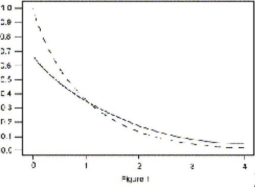
10 Instances of variables with restricted range are numerous, and an outstanding family of examples is connected with lifetimes. In parametric statistics, a very simple model would start with the exponential distribution.

Assume that the old treatment X is distributed as an exponential with failure rate $1/\lambda$ (and hence with mean $\lambda$, and that the new treatment Y is also exponential, but with failure rate $1/\lambda$ (with $1/\mu \text{}<1/\lambda$). Since the exponential distribution is determined by a single parameter, the difference between the two populations could be specified by a difference in means $\Delta =\mu \text{}\text{}\text{}\text{}-\text{}\lambda$. Hence, for a fixed type of distribution (exponential), one could formulate a test in terms of an increase in means only ($H_0:\Delta \text{}\text{}=\text{}0$ versus $H_1:\Delta \text{}\text{}>\text{}0$), while the densities do not display a constant shift and $Y\underset{\_}{\underset{\_}{d}}X+\text{}\Delta$ does not hold (Figure 1).

Figure 1. Comparison of two exponential densities, one with mean $\lambda$= 1 (dotted line) and the other with mean $\mu$= 1.5 (solid line).

11 The above properties of the exponential are, of course, well-known. Engineers, when studying reliability problems, often use the exponential and model a change as a ratio $\theta =\mu /\lambda$. Turning to the nonparametric analogue, biostatisticians look for instances where proportional hazards are a plausible assumption for modeling survival data in clinical trials. Here, also, longer survival times are not modeled as a “constant additive shift.”

3. A Nonparametric Framework

12 For many students, comparing two treatments the nonparametric way reduces to clicking “Wilcoxon” instead of “Student t” in a statistical computer package or replacing mean by median in a report. This often reflects an almost automatic transposition of the parametric model to the nonnormal situation, again restricting attention to one number, be it the median in this case. Abandoning the normality assumption, however, allows one to abandon the induced shift model altogether. It invites one to delve a bit deeper into the understanding of basic model properties of the treatments one wants to compare. The context of the Wilcoxon test can be an ideal starting point for this mental exercise.

13 How much flexibility can be incorporated into a nonparametric “new better than old” statement, while still ending up with a treatable expression? The classical answer to this question (see, e.g., Lehmann 1998, p. 66, or Bickel and Doksum 1977, p. 345) involves stochastic ordering, and this topic deserves ample explanation when students are exposed to it for the first time. If X stands for the (population of outcomes of the) old treatment and Y for the new one, one could define “new better than old” as Y is stochastically larger than X. Denoting the cumulative distribution functions (c.d.f’s) of X and Y by F(·) and G(·), the stochastic ordering is expressed as “F(x) $\ge$ G(x) for all x, with F(x) > G(x) for at least one x.” Most textbooks warn the students here of the apparent mistake in the direction of the inequality sign, essentially telling them that up until now, they haven’t given the interpretation of a cumulative distribution function enough thought.

14 A definition of “stochastically larger than” will not be very helpful unless students are able to relate this concept to familiar situations. Well-chosen examples and pictures are crucial here. We illustrate this with some useful pictures and descriptive phrases, starting with the well-known shift model.

4. The Classical Shift Model

15 The two-sample location problem is one of the most widely studied problems in mathematical statistics. Restricting attention to shift models $Y\underset{\_}{\underset{\_}{d}}X+\text{}\Delta$ (or $G(x)=F(x-\Delta )$), nice optimality properties of specific tests have been proved (e.g., the t-test is uniformly most powerful for a normal shift, and the Wilcoxon test is locally most powerful for a logistic shift). However, for all shift models, one should keep in mind that testing $H_0:\Delta \text{}\text{}=\text{}0$ versus $H_1:\Delta \text{}\text{}>\text{}0$ (or $\Delta <\text{}0$ or $\Delta \text{}\ne 0$) reflects one’s belief that the improvement in the new treatment shows itself in a “constant additive” way.

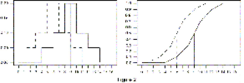
16 The improvement in the outcomes of the new treatment is a fixed quantity $\Delta >\text{}0$ added (in a probabilistic sense) to the outcomes of the old treatment, and this property holds uniformly over the whole range of the experiment (Figure 2). Formulated in this way, the implication of a shift model seems rather drastic, and students at this point start having a hard time believing that any of their own experiments will ever comply with such a model. Some of them might even confess that they had not previously given the idea of constant additivity any consideration while routinely carrying out two-sample t-tests.

Figure 2. The Shift Model. The solid lines represent the density (left) and c.d.f. (right) of the new treatment $Y\underset{\_}{\underset{\_}{d}}X+\text{}\Delta$ . The improvement is additive and constant over the whole range of observable outcomes.

5. Location and Stochastic Ordering

17 A natural way to allow more flexibility in modeling “new better than old” gives rise to $Y\underset{\_}{\underset{\_}{d}}X+\text{}\Delta (x)$ with $\Delta (x)\ge \text{}0$ for all x and strict inequality for at least one x (Figure 3). The special case $\Delta (x)\equiv \text{}\Delta >\text{}0$ reduces to the shift model.

Figure 3. Stochastically Larger Than. The solid lines represent the density (left) and c.d.f. (right) of the new treatment $Y\underset{\_}{\underset{\_}{d}}X+\text{}\Delta (x)$. The flexibility of modeling a new treatment as the one with higher outcomes is illustrated by the solid c.d.f., which only has to stay below the dashed one.

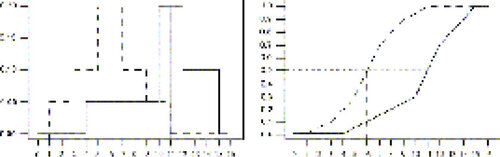
18 Writing $Y\underset{\_}{\underset{\_}{d}}X+\text{}\Delta (x)$ clearly shows that one expects higher values for the new treatment, allowing at the same time for dependence of the degree of improvement on the value at hand. This model makes sense for a variety of experiments. It essentially replaces “Y is stochastically larger than X” by the following sentence which is usually better understood: “For any fixed value x₀, the probability that the new treatment yields outcomes higher than x₀ is bigger than the probability that the old treatment yields outcomes higher than x₀.”

19 Note that the above model is also handy for teaching testing procedures in more specialized settings. A notable example is $Y\underset{\_}{\underset{\_}{d}}X+\text{}\Delta (x)$ with $\Delta (x)=\text{}ax$ for a > 0 and X a positive random variable (lifetime), modeled by the exponential. The nonparametric analogue in this case leads to the (simple) proportional hazards model, a subclass of the “stochastically larger than” model for which the Savage - Exponential Scores - Logrank test is the statistical method of choice.

20 It might be worthwhile in its own right to acquaint students with the concept of “stochastically larger than” through simulation. Start with a distribution of X and a deterministic function $\Delta (x)\ge \text{}0$, not everywhere zero.

Take a random sample X₁, X₂, …, X_m from the X population. Then, independently of the first sample, take another random sample X₁, X₂, …, X_n from X and construct Y₁, Y₂, …, Y_n through $Y_i=X_i\text{}+\text{}\text{}\Delta \text{}\text{}\text{}\text{}\text{}(X_i)$for the second sample. This procedure may help to make clear the notion that there has been an intervention so that Y is “improved” over X. At the same time it clearly shows that “Y tends to be larger than X” must be understood in a probabilistic sense.

6. The Reparameterization Fallacy

21 Pictures like those in Figure 2 and Figure 3 acquaint students with the “stochastically larger than” model. At this point, however, some students intuitively go back to numbers, remarking that in both pictures the median of the new treatment is clearly the larger one. So why not formulate the test as $H_0:{\theta }_Y\text{}\text{}=\text{}\text{}{\theta }_X$ versus $H_1:{\theta }_Y\text{}\text{}=\text{}\text{}{\theta }_X$ with Ɵ the median?

22 Another common observation is that if the probability of exceeding any x₀ is bigger for the new treatment than for the old one, then P(Y > X) > .5, whereas P(Y > X) = .5 if there is no treatment effect. So why not formulate the test as H₀: P(Y > X) = .5 versus H₁: P(Y > X) > .5?

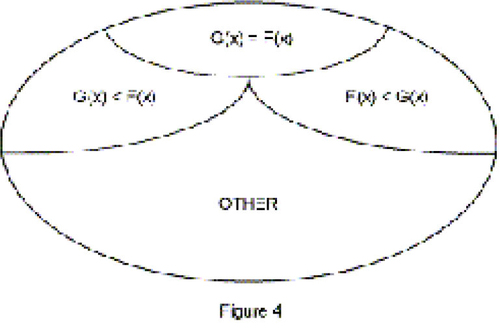
23 At this point, Figure 4 is crucial, showing that the stochastic ordering is only a partial one, and hence that models based on this ordering cannot be collapsed into statements about simple numbers.

Figure 4. Stochastic Ordering. The most important subset might be “OTHER,” indicating that the stochastic ordering is only a partial one that cannot be fully captured by the ordering of numbers.

24 Extra insight is provided by Figure 5, which shows that new can be better than old even when they have the same median, and Figure 6, which shows that the median of a new treatment can be substantially larger than that of an old treatment, even though the old treatment performs better in (possibly important) tail regions.

Figure 5. Stochastic Ordering and Median. The new treatment (solid line) has the same median as the old treatment, while nevertheless being strictly superior almost everywhere.

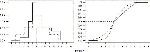
Figure 6. A Misleading Median. The median of the new treatment (solid line) is clearly larger than the median of the old treatment, even though the old treatment outperforms the new one in (possibly important) tails.

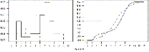
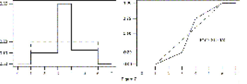
25 An analogous argument holds for P(Y > X), and, furthermore, one can construct examples where P(Y > X) = .5 but ${\theta }_Y\ne \text{}\text{}\text{}{\theta }_X$ or where ${\theta }_Y=\text{}\text{}\text{}{\theta }_X$ but P(Y > X) > .5. A claim that P(Y > X) > .5 reflects superiority of the new treatment could be hard to relate to by the student who is convinced that for almost half of the outcome range the old treatment outperforms the new one (see Figure 7). Thinking that P(Y > X) = .5 is one of the many equivalent ways of saying that there isn’t any difference between new and old can be misleading too (see Figure 8).

Figure 7. P(Y > X) and Superiority. The new treatment Y (solid line) fulfills P(Y > X) > .5, although the old treatment X is superior in almost half of the outcome range.

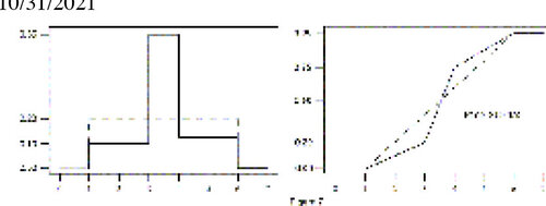
Figure 8. P(Y > X) and Equality. That P(Y > X) = .5 reflects the equivalence of two treatments is certainly not true, as illustrated by this figure where P(Y > X) is exactly equal to .5. The new treatment Y is represented by the solid line.

26 When studying specific properties of a particular experiment, there might be a good reason for formulating the research question strictly in terms of the median (or in terms of P(Y > X)). However, one should then realize that in nonparametric models, two distributions need not be equal under the null hypothesis if it is stated as $Y_0:\text{}{\theta }_i\text{}=\text{}\text{}{\theta }_X$ (see Figure 5). The null distribution of the WMW statistic (and more generally, of a permutation statistic) can then no longer be determined since the nice and simple nonparametric distribution of the sum of the treatment ranks stems from the basic assumption that treatment and control are identically distributed under the null hypothesis.

27 When a problem is formulated in terms of medians, while assuming implicitly that the distributions have the same shape, this assumption should be mentioned explicitly, leading to a null hypothesis of the form G(x) = F(x). In fact, even the nonparametric Behrens-Fisher problem (see Lehmann 1991, p. 323), where the two populations are modeled as $F((x-\xi )/\sigma )$ and $F((y-n)/\tau )$, does not justify the use of WMW for testing $H_0:\text{}\xi \text{}\text{}\text{}=\text{}\text{}\eta$. Indeed, G(x) = F(x) is not guaranteed under the null hypothesis, nor is stochastic ordering under the alternative hypothesis.

7. Exploring the Literature

28 Not many textbooks pay ample attention to explicitly stating the underlying model, before indulging in the Wilcoxon-Mann-Whitney test procedure. Formulation of hypotheses in the collapsed way (e.g., on the median) is not always put in its shift model framework, nor is the necessity for such a model motivated. Mixing stochastic and numerical ordering leads to amazing statements and sloppy expressions, especially for two-sided tests. When students explore standard textbooks such as Conover (1980), Gibbons and Chakraborti (1992), Hollander and Wolfe (1973), Lehmann (1998), Noether (1991), Randles and Wolfe (1991), and Siegel and Castellan (1988), they will encounter examples of the three situations described in Sections 7.1, 7.2, and 7.3.

7.1 A Precise Formulation

29 As mentioned above, stochastic ordering must be treated carefully in the formulation of hypotheses, with special attention to two-sided tests. Examples of carefully stated hypotheses are

H₀: G(x) = F(x) versus H₁: G(x) ≤ F(x) with inequality for at least one x (new is better than old),

H₀: G(x) = F(x) versus H₁: G(x) ≥ F(x) with inequality for at least one x (new is worse than old), and

H₀: G(x) = F(x) versus H₁: either G(x) ≤ F(x) or G(x) ≥ F(x) with inequality for at least one x (new differs from old in the sense that it is either stochastically larger than old or that it is stochastically smaller than old (see again Figure 4)). Hypotheses formulated in this way can be found, e.g., in Lehmann (1998) and Noether (1991).

7.2 A Restricted Formulation

30 Several textbooks present the WMW test in a restricted setting, but only some mention this setting explicitly. If one is convinced that the improvement can be modeled as a shift, a formulation of the test as $H_0:\text{}{\theta }_Y\text{}\text{}\text{}=\text{}\text{}{\theta }_X$ versus $H_1:\text{}{\theta }_Y\text{}\text{}\text{}>\text{}\text{}\text{}{\theta }_X$ (or ${\theta }_Y\text{}\text{}\text{}<\text{}\text{}\text{}{\theta }_X$ or ${\theta }_Y\text{}\text{}\ne \text{}\text{}\text{}{\theta }_X$) creates no particular problem for the use of the WMW

statistic. Some textbooks do indeed draw attention to the restricted framework of a shift model, but others do not. As mentioned above, p-values computed for a WMW test based solely on the assumption $H_0:\text{}{\theta }_Y\text{}\text{}\ne \text{}\text{}\text{}{\theta }_X$ about medians can be completely wrong.

7.3 Some Confusion

31 When one agrees that a nonparametric framework naturally calls for hypotheses on ordered distribution functions rather than on parameters, it should be kept in mind that a stochastic ordering is only partial. A two- sided test should reflect this.

32 Typical confusion arises from intermingling stochastic ordering and numerical ordering, as shown in the following statement where a two-sided test for stochastically ordered alternatives was intended:

H₀: F(x) = G(x) for all x

H₁: F(x) ≠ G(x) for some x

It is clear that the class of alternatives is much too broad here. Similar problems may arise in “reparameterized” statements such as H₁: P(Y > X) ≠ .5 or $H_1:\text{}{\theta }_Y\text{}\text{}\ne \text{}\text{}\text{}{\theta }_X$, if additional assumptions on the underlying distributions are not specified.

8. Conclusion

33 For comparing two treatments, the t-test should be included in an applied statistics course. But should the t- test be the first (and sometimes the only) statistical procedure that students see? Or should one start with a nonparametric framework and dare to spend an increased amount of teaching time on underlying model assumptions illustrated with ample pictures and descriptive phrases? After all, students should learn that in the design and analysis of a real-world experiment, the first thing to think hard about is the experiment. Its expected behaviour, plausible properties, and the differences of interest all play a crucial role in the formulation of the research question and, consequently, in the selection of an appropriate test statistic. An overemphasis on the widely used t-test can give the impression that a location difference between two treatments must be modeled as a shift.

34 Considering the non-monotonicity, the sensitivity to outliers, the small gain in efficiency when the underlying model really is a normal shift, and the constant additivity formulation of the t-test, one is forced to agree with Noether (1991, pp. 134-135), who wrote: “Quite a number of statisticians, …, are convinced that there are rarely, if ever, sound statistical reasons for preferring the t-test to the Wilcoxon test.”

Acknowledgments

Discussions with D. P. Harrington (Harvard School of Public Health) were very helpful while preparing this paper. Constructive remarks made by the referees are gratefully acknowledged. Substantial help from the Editor greatly improved the readability of the paper.

References

- Bickel, P. J., and Doksum, K. A. (1977), Mathematical Statistics: Basic Ideas and Selected Topics, Englewood Cliffs: Prentice Hall.
- Conover, W. J. (1980), Practical Nonparametric Statistics (2nd ed.), New York: Wiley
- Gibbons, J. D., and Chakraborti, S. (1992), Nonparametric Statistical Inference ( 3rd ed.), New York: Marcel Dekker.
- Hollander, M., and Wolfe, D. A. (1973), Nonparametric Statistical Methods, New York: Wiley.
- Lehmann, E. L. (1991), Testing Statistical Hypotheses ( 2nd ed.), Pacific Grove: Wadsworth & Brooks/Cole.
- Lehmann, E. L.– (1998), Nonparametrics: Statistical Methods Based on Ranks ( revised 1st ed.), Upper Saddle River, NJ: Prentice Hall.
- Noether, G. E. (1991), Introduction to Statistics: The Nonparametric Way, New York: Springer-Verlag.
- Randles, R. H., and Wolfe, D. A. (1991), Introduction to The Theory of Nonparametric Statistics (reprint ed. w/corrections), Malabar, FL: Krieger.
- Siegel, S., and Castellan, N. J. (1988), Nonparametric Statistics for the Behavioral Sciences ( 2nd ed.), New York: McGraw-Hill.