A Teaching Tool for Nonlinear Regression: Visual Fit

Abstract

We describe a Java applet that allows users to see and learn the fitting of regression models in a manner that is both visual and interactive, as well as consonant for linear and nonlinear models. In addition, this program familiarizes users with the fact that many different parameterizations exist for a single function, and it provides insight about the relationship between these models. Called Visual Fit, this program draws scatterplots of data and allows users to fit various nonlinear models to the data. The program can also provide least squares estimates or true population parameters for comparison with the estimates made by the user. We discuss what types of parameters can be represented in a visually obvious way and which cannot. Visual Fit may be useful for both introductory statistics classes and higher-level courses. Visual Fit is available at http://www.amstat.org/publications/jse/secure/v7n2/visualfit.html

Keywords:

• Interactive
• Java applet
• Web-based

1. Introduction

1 Nonlinear least squares regression is the fitting of a model to data, where the model parameters are related to the explanatory variable(s) in a fashion that is not linear. On a conceptual level, nonlinear least squares works primarily the same way as linear least squares; estimates of model parameters are obtained by finding the set of parameters that minimizes the sum of squared deviations between the data and model (hence the name least squares). Nonlinear least squares is more complicated only because it is usually not possible to obtain these estimates algebraically; closed-form expressions for nonlinear least squares estimators are often impossible to find. Instead, numerical search procedures are typically used, which arrive at least squares parameter estimates through computationally intensive methods. Therefore, nonlinear least squares computations are almost always done by computer.

2 This extra complication is one of the main reasons why many statistics courses and textbooks have little or no coverage of nonlinear least squares (e.g., Ott 1993, Snedecor and Cochran 1989, Moore and McCabe 1993, Devore and Peck 1993). As a result, nonlinear regression is often neglected in statistics courses, even though nonlinear regression is widely used in applied research. Many statistics students therefore have little exposure to this kind of regression and might regard nonlinear regression as something of an enigma.

3 Currently there exist interactive applications that allow regression concepts to be learned on the computer. An example is ActivStats, developed by Data Description, Inc. Users can explore straight-line regression with the ActivStats “Least Squares Tool.” In this program, users learn about the least squares criterion for fitting lines by dragging the line’s slope and intercept with the mouse. The equation and sum of squared residuals are displayed and automatically updated. ActivStats can then show the true least squares line for comparison.

4 The aim of this project was to develop a computer program that extended this method of teaching least squares fitting to encompass nonlinear models, as well as linear models. This lets users see least squares fitting on a broader scale – one which is not restricted only to straight-line regression. In addition, this program familiarizes users with the fact that many different parameterizations exist for a function, and it provides some insight about the relationship between these models.

5 This program, called Visual Fit, draws scatterplots of data and allows users to fit various linear and nonlinear models to the data. The program itself also fits the data by making use of a nonlinear least squares algorithm. Visual Fit has been developed in order to allow students to have a good visual sense for nonlinear least squares and to see that nonlinear regression and linear regression are conceptually the same. Visual Fit was written in Java (see Program Usage section) in order to allow compatibility with various platforms, as well as for easy portability to the Web.

6 Visual Fit can be useful for both introductory statistics classes and higher-level courses. Part of Visual Fit’s value lies in its ability to allow students to perceive the overall concept of least squares. Furthermore, the material taught by Visual Fit need not add to an already over-packed curriculum; it can certainly be used as a supplemental tool. Students can be free to explore least squares on their own using Visual Fit.

7 This paper consists of the following sections:

•	Program Performance describes how the program works in general.
•	Nonlinear Least Squares Algorithm discusses the method used by the program to find least squares estimates.
•	Regression Functions in the Program describes what models and parameterizations were used in the program and how they were represented.
•	Program Structure describes the basic class structure of the program.
•	Program Usage contains instructions on using the program.
•	Discussion and Conclusions describes some interesting and important findings.

2. Program Performance

8 The basic operation of this program is as follows: generate a set of data using a specific regression model with randomly selected parameter values plus error. This dataset is displayed along with a “trial fit.” The parameters can then be controlled by the user in an attempt to best fit the data. These parameters may be modified either by inputting new parameter values through the keyboard or by graphically manipulating “parameter box” representations using a mouse. We will have more to say about the visual representation of a parameter in later sections. Different functions and parameterizations may be used to fit the data. The functions and their parameterizations, as well as the methods of representation, are described in further detail in the section entitled Regression Functions in the Program.

9 The program responds to any change in parameters by redrawing the trial fit and calculating the new sum of squared differences between the data and the user-controlled function. When the user has finished fitting the model, the actual least squares estimate (see the next section) or the true population parameters and the user’s guess are then displayed simultaneously for comparison.

3. Nonlinear Least Squares Algorithm

10 In this program, the method used to calculate least squares estimates is the Levenberg-Marquardt method, also known as the Marquardt method (Press, Teukolsky, Vetterling, and Flannery 1992). This method works well in practice and is a commonly used technique for nonlinear least squares.

11 For a specified model f with parameters a to be estimated, we will use the following notation: $$Y_i\text{}=\text{}f(X_i,a)\text{}\text{}\text{}+{\epsilon }_i\text{}\text{}\text{}\text{}\text{}a\text{'}=[a_1,\mathrm{\dots },\text{}\text{}aM]\text{}\text{},$$

where Y_i is the value of the response variable in the ith observation, X_i is the value of the predictor variable in the i^th observation, and ε_i is the error term in the i^th trial. Visual Fit will, with each new iteration of the algorithm, evaluate the sum of squared differences between the data and the model: $$Q(a_p)\text{}\text{}=\text{}{\displaystyle \sum _{i=1}^n{(Y_i\text{}-\text{}f(X_i,\text{}\text{}\text{}{a}_p))}^2,}$$

where a_p is the parameter estimates for the pth iteration. For the initial guess a₀, Visual Fit uses the true values of the parameters that were used to generate the dataset.

12 A rule for termination of the routine is also necessary. This program uses the following condition for stopping (suggested by Kennedy and Gentle 1980): $$0\text{}\le Q(a_p)-Q\text{}(a_{p+1})\text{}\text{}<\tau$$

That is, terminate at the p+1th iteration whenever the sum of squares decreases by an amount less than some tolerance . Other stopping rules (Kennedy and Gentle 1980) considered were: $$\underset{K}{\max }\text{}\text{}\left|{\beta }_k\right|\text{}<\tau ,$$

which terminates when the gradient of the sum of squares with respect to each parameter is small enough, and $$\left|\right|\beta \left|\right|<\tau ,$$

which terminates when the norm of the gradient of the sum of squares with respect to each parameter is small enough. However, these criteria were found to behave badly from time to time. More specifically, situations arose where it was impossible to meet these criteria, causing the program to loop endlessly.

13 The Levenberg-Marquardt algorithm was implemented in the program with the following settings:

•	The starting value of $\lambda$, the mediating factor between Gauss-Newton and Steepest Descent, was 0.001.
•	The factor $\gamma$ by which to change $\lambda$was 10.
•	The tolerance $\tau$for stopping rule was 0.00001.

The starting value of $\lambda$ and the factor $\gamma$ were suggested by Press et al. (1992). The tolerance $\tau$ was adjusted so that it was small enough to ensure accurate estimates, but not so small that the program took too long to complete the algorithm.

4. Regression Functions in the Program

14 Table 1 lists all of the regression functions and their parameterizations used in the program. Models included in Visual Fit were ones whose parameters (a) made physical sense and could be interpreted by the user in a logical manner, and (b) could be represented by the program in a way that accurately depicted the parameter’s meaning. For example, the following logistic model has parameters that are sufficiently understandable and representable: $$f(x)\text{}=\frac{a}{1+e\frac{4m}{a}(x_h-x)}$$

This parameterization is included in Visual Fit. As described in Table 1, a represents the maximum height of the function, x_h is the value of x at which the function equals a/2, and m represents the slope of the function at x = x_h.

Table 1. List of Functions and Parameterizations Used in Visual Fit

Function	Parameterization	Description of Parameters
Linear	$f\left(x\right)=a+bx$	a - y-intercept b - Slope of the line
	$f(x)\text{}\text{}=\text{}a+b(x-\overline{x})$	a - Height of the function at $x=\overline{x}$ b - Slope of the line
Quadratic	$f(x)\text{}\text{}=\text{}a+b(x-\overline{x})+c{(x-\overline{x})}^2$	a - Height of the function at $x=\overline{x}$ b - Slope of the function at $x=\overline{x}$ c - Quadratic effect
Exponential	$f(x)\text{}\text{}=\text{}a(1-e^{-bx})$	a - Maximum height of the function b - Rate of approach towards a
	$f(x)\text{}\text{}=\text{}a(1-2^{-x/xh})$	a - Maximum height of the function xh - Value of x at which the function equals a/2
	$f(x)\text{}\text{}=\text{}a(1-e^{-dx/a})$	a - Maximum height of the function d - Slope of the function at origin
Exponential with Intercept	$f(x)\text{}\text{}=\text{}a(1-e^{-bx})+c$	a - Maximum height (from c) of the function b - Rate of approach towards a c - y-intercept
	$f(x)\text{}\text{}=\text{}a(1-2^{-x/xh})+c$	a - Maximum height (from c) of the function xh - Value of x at which the function equals a/2+c c - y-intercept
	$f(x)\text{}\text{}=\text{}a(1-e^{-dx/a})+c$	a - Maximum height (from c) of the function d - Slope of the function at origin c - y-intercept
Logistic	$f(x)\text{}\text{}=\text{}\frac{a}{1+e^{\frac{4m}{a}(x_h-x)}}$	a - Maximum height of the function xh - Value of x at which the function equals a/2 m - Slope of function at ^x ^= xh

15 Under a different parameterization, the logistic model may be more difficult to interpret. In this second model, shown below, the parameters are more difficult to represent and interpret: $$f(x)\text{}=\frac{a}{1+e-(b+cx)}$$

Parameters b and c do not have a physical interpretation that is sufficient for representation within Visual Fit. Therefore this parameterization was not included in the program.

16 The definition and behavior of a parameter are conveyed to the user by (a) the movement of the parameter box, (b) description of the parameter which may be brought up in the message area at any time, and (c) reference lines that may be drawn on the graph to convey some relationship between the graph and a parameter. (Reference lines are gray in color; lines that convey a mathematical interpretation are pink.) Representation of a parameter will consist of these elements. Together they help the user understand the parameters in the model.

17 Certain kinds of parameters that are similar in nature are represented by Visual Fit in the same way. Some may have an obvious method of representation. Parameters that denote some specific x or y value related to the function are the easiest to represent. For example, the parameter a of the linear model $$f\left(x\right)=a+bx$$

represents the y-intercept, or value of y where x = 0. This is simply controlled by a parameter box which lies on the point where the line crosses the y-axis and moves only vertically. Another example is the parameter x_h of the model $$f\left(x\right)=a(1-e-x/xh).$$

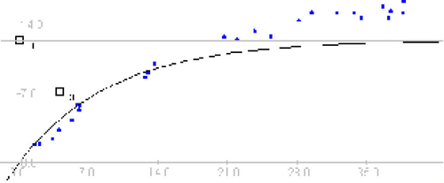
x_h represents the x value at which the function is equal to a/2. This parameter is controlled by a box that moves along the x-axis. Reference lines are drawn on the graph to show the relationship between the parameter box and the function (Figure 1).

Figure 1. Horizontal Reference Lines. Reference lines are drawn on the graph to help convey the meaning of the parameters.

18 Similarly, parameters that represent lengths in the scale of x or y are represented by placing the parameter box on one end of the length that the parameter denotes. In the model $$f\left(x\right)=a(1-e^{-bx})+c,$$

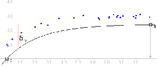
the parameter a represents the length on the y scale between the function’s height at x = 0 and the asymptote approached by the function as x approaches infinity. In this case, a box is placed at the asymptote, y = a + c, and the length it represents is labeled on the graph (Figure 2).

Figure 2. Vertical Reference Lines. The vertical reference line indicates the distance represented by parameter a.

19 Parameters that denote the derivative or slope at a certain point on the function are a little bit more complicated. Slope parameters are controlled by parameter box controls that move in a circle around a set point on the function. All slope parameters are controlled this way. This will let users see the similarity between the slope of a straight line and one from a more complex model.

20 Other function parameters may be more difficult to portray. One of the more complicated representations was used in the exponential model $$f\left(x\right)=a(1-e^{-bx}).$$

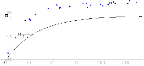
In this parameterization, the parameter b may be difficult to interpret. Users may understand by inspection or manipulation that b is somehow responsible for how quickly the function approaches its asymptote, but they may not have a physical perception of its relationship to the function. In this case we have decided to let users see the parameter b as a quantity that is proportional to the ratio between two lengths on the y scale, a - f(x₁) and a - f(x₂), where x₁ and x₂ are arbitrary values for x that are close together. This relationship was an approximation taken from the differential equation by which b was originally defined in this model: $$\begin{array}{c}b=-\frac{d}{dx}\log (a-f(x))\\ =-\frac{1}{a-f(x)}\frac{d}{dx}(a-f(x))\\ \approx -\frac{(a-f(x_1))-(a-f(x_2))}{\Delta x(a-f(x_1))}.\end{array}$$

while b is more naturally interpreted on a different scale (the log of a - f(x)), this representation of b allows its interpretation on the x-y scale. These lengths are indicated by two pink lines. The parameter box controls the length of a - f(x₁), the numerator of this ratio of lengths. The parameter description indicates the relationship described (Figure 3).

Figure 3. Representation of a Complicated Parameter. In this model, f(x) = a(1 - e-bx), the parameter b is described as a ratio between the lengths of the two pink lines.

21 Obviously, there may be many different ways to represent a parameter. The choice of how a parameter is to be depicted should involve a decision about what aspect of the parameter’s behavior we would like to elucidate, and whether this aspect can be illustrated by parameter box controls. In deciding upon a method of representation, care should be taken not to use any depiction that is more descriptive of some other parameterization of the same function. Such a representation would not be an accurate portrayal of the actual parameter being changed.

5. Program Structure

22 This program was written in Java, an object-oriented language that was developed and released by Sun Microsystems, Inc. in 1995. Java has received much attention from the business community, due to its innovative ability to run dynamically from Web pages. Java was chosen primarily for its robust nature; it was possible to perform tasks through Java a number of different ways. Java programs are easily placed on Web pages and are also extremely platform independent; that is, they can be run on different operating systems. Other development platforms were considered, such as C++ and Lisp-Stat. These languages have implementations that would have made the graphics and computations in VisualFit easier. However, we decided to use Java for its superior compatibility across platforms and the fact that all major Web browsers have a Java run-time. (We discuss some of the difficulties associated with Java in the Discussion and Conclusions section.)

23 A copy of this program’s code is available at the Visual Fit Web page (see the next section). The program’s basic structure is composed of three main object-oriented classes: VisualFit, Function, and Graph. Graph handles the drawing of the graph, Function houses all of the variables and methods pertaining to the data, the trial fit, and each of the regression models and associated details (e.g., partial derivatives, parameter values, location of parameter boxes), and VisualFit holds the entire program together by controlling communication among all of the classes. Table 2 provides a brief description of each class. These classes are defined in files called Java class files. All are necessary for the program to execute correctly.

Table 2. List of Java Classes Comprising Visual Fit

Class name	Description
VisualFit	Main body of program. Handles most user actions.
Function	Performs all of the actions specific for the data, the trial fit, and each regression model.
Graph	Manages the scatterplot graph. Also controls the mouse interface with parameter box controls.
ControlPanel	Manages the control panel next to the graph.
Convert	Converts back and forth between the graph’s continuous coordinates and the screen’s pixel coordinates.
Format	Controls number formatting (written by Cay Horstmann, Sun Microsystems, Inc.).
MessageArea	Controls the message panel on the side.
SSBar	Calculates and draws the sum of squares bar.
ArrayOp	A set of functions used for manipulating arrays.
VisualFitFrame	A frame that houses the applet in VisualFit. Only used when program is run as a stand-alone.
Generate	Performs all of the necessary random number generation.
Sort	Performs all of the necessary data sorting.

6. Program Usage

24 This program can be run locally on a computer by obtaining all 12 class files (listed in the previous section) and a Java interpreter, which is a program that is able to run Java programs by interfacing with Java class files.

Sun Microsystems’ Java Development Kit (JDK) is an example of such a program.

25 However, the easiest way to run the program is to execute it as an applet, or, in other words, to access the program through a Web browser such as Netscape Navigator. Visual Fit is available at http://www.amstat.org/publications/jse/secure/v7n2/visualfit.html

Click on “Start Visual Fit,” and the program will begin. This method will work from a Web page as long as the Web browser is Java compliant. Most users will not have a problem with this; almost all Web browsers have Java capabilities.

26 It should be noted that, on slower machines, users may experience a slight lag whenever parameter box controls are moved. Visual Fit was written and tested primarily on a Windows 95 platform. Other platforms seem to have no trouble running Visual Fit. However, performance on these platforms has not been tested as extensively. It should also be noted that when the program executes under a Web page, performance may be worse than when running the program locally. Specifically this refers to the lag of parameter box controls mentioned previously.

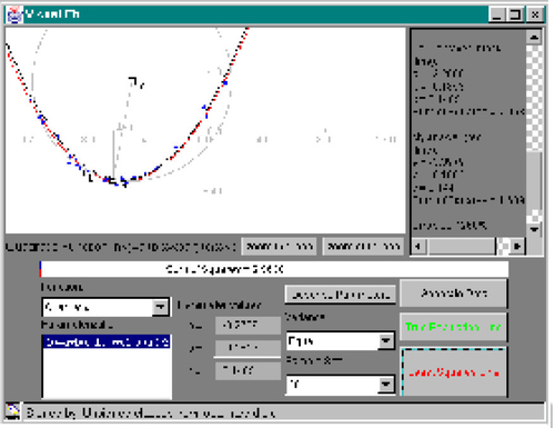
27 When the program starts, a dataset and model are immediately displayed (Figure 4). Fit the dataset by changing the values of the parameters in the model. This can be done by either dragging the parameter box controls or by typing new values on the control panel (Figure 5). The sum of squares is displayed so that the user may observe the effect of changing the parameters and gauge the quality of the fit. When finished fitting the model to the data, click on the “Least Squares Line” button. The program will display the actual least squares solution (calculated using Levenberg-Marquardt) as a red line on the same graph as the user’s trial fit. The message area on the side displays a comparison between the two fits (Figure 6). To look at another dataset, click on “Generate Data.” The program will generate another dataset using the same model.

Figure 4. Start of the Visual Fit Applet.

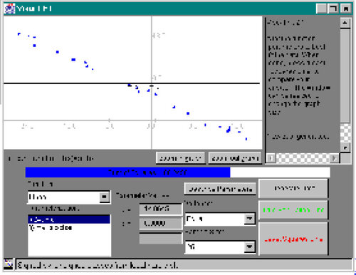
Figure 5. Changing Model Parameters. Parameters may be controlled by dragging their corresponding parameter box controls.

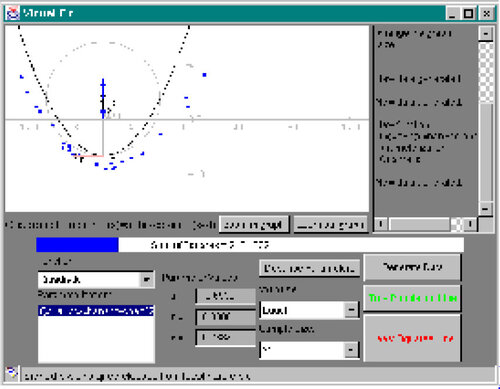
Figure 6. Comparison With Least Squares. Users’ estimated parameters can be compared with least squares estimates.

28 Similarly, clicking the “True Population Line” button will cause Visual Fit to display the actual line used to generate the dataset. This can help users to understand the difference between the true population line and the least squares line.

29 Different parameterizations of the functions may be selected from the “Parameterization” list. Visual Fit will automatically convert all parameters. This can be done either before or after the answer is displayed. A description of these parameterizations may be viewed at any time by clicking on “Describe Parameters.” The descriptions appear in the message area on the side.

30 To switch to a different regression function, choose from those listed in the “Function” pull-down menu. The program will respond by updating the trial function and the values displayed in the bottom panel.

31 The scale of the graph can be changed at any time by clicking on the rescaling buttons located below the graph. This should be done if the user finds fitting the function to be easier at a different graph scale.

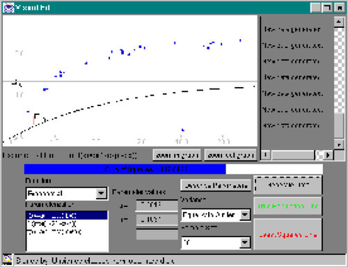
32 Additional features of Visual Fit include a choice of sample size and error distribution. Users can have the program generate datasets with errors that are not i.i.d. normal. For example, datasets with extreme outliers may be generated (Figure 7).

Figure 7. A Dataset With an Outlier. Outliers and other irregularities may be generated.

7. Discussion and Conclusions

33 The fact that Java is a very new language and is still undergoing constant change meant that its graphical user interface capabilities were somewhat limited, when compared with other development platforms, such as Visual C++ or Visual Basic. Visual layout of the program turned out to be surprisingly difficult, and certain features, such as spin buttons and print capability, were unavailable. It should be noted that Java 1.1 (and above) does address some of the problems mentioned above, such as printing. However, Visual Fit was written using Java 1.0.2, a less-than-current version. This was done so that Visual Fit would enjoy compatibility with a broader range of Web browsers, since some browsers do not support the new version of Java (e.g., Netscape 3.0 and lower).

34 It was observed that there was an occasional lack of convergence from the Levenberg-Marquardt algorithm when the data were not generated from the model being fit. However, this is infrequent if the user makes a minimally reasonable guess, since the applet uses the inputted parameters as a starting point for the algorithm.

35 This program uses the model parameters from which the data were generated as the values for a₀, the initial guess at the parameters for Levenberg-Marquardt. This was a natural choice for a₀; the generation parameters are almost always a very good guess for the least squares estimates. However, in the extremely exceptional case that the user’s estimate provides a smaller sum of squares than the one initially calculated, Visual Fit will use the user’s inputted parameters for a₀^.

36 For parameters of many models, providing an interpretation on the scale of the graph was often extremely difficult. Other parameters cannot be represented this way at all. For a particular model, we needed to consider whether Visual Fit would be able to explain the parameters to users in the manner intended. If the intention is to explain the parameters on a completely different scale, or if the graph-scale interpretation is too complex to provide a good understanding of the parameter’s meaning, then these parameters are not well-explained by the methods employed by Visual Fit. Models with these parameters were not included in the program.

37 While nonlinear regression computations are relatively difficult, this program can help students to see that the main ideas behind linear model fitting also apply to nonlinear model fitting. This program attempts to concentrate more on the similarities between the two, rather than the extra difficulties associated with nonlinear regression. Students will see that linear regression and nonlinear regression are alike on a conceptual level.

References

- Devore, J., and Peck, R. (1993), Statistics: The Exploration and Analysis of Data (2nd ed.), Belmont, CA: Duxbury Press.
- Kennedy, W. J., and Gentle, J. E. (1980), Statistical Computing, New York: Marcel Dekker.
- Moore, D. S., and McCabe, G. P. (1993), Introduction to the Practice of Statistics (2nd ed.), New York: W. H. Freeman and Company.
- Ott, R. L. (1993), An Introduction to Statistical Methods and Data Analysis (4th ed.), Belmont, CA: Duxbury Press.
- Press, W. H., Teukolsky, S. A., Vetterling, W. T., and Flannery, B. P. (1992), Numerical Recipes in C: The Art of Scientific Computing (2nd ed.), New York: Cambridge University Press.
- Snedecor, G. W., and Cochran, W. G. (1989), Statistical Methods (8th ed.), Ames, IA: Iowa State University Press.