Getting What You Pay For: The Debate Over Equity in Public School Expenditures

Abstract

Using data from the 1997 Digest of Education Statistics, this teaching case addresses the relationship between public school expenditures and academic performance, as measured by the SAT. While an initial scatterplot shows that SAT performance is lower, on average, in high-spending states than in low-spending states, this statistical relationship is misleading because of an omitted variable. Once the percentage of students taking the exam is controlled for, the relationship between spending and performance reverses to become both positive and statistically significant. This exercise is ideally suited for classroom discussion in an elementary statistics or research methods course, giving students an opportunity to test common assumptions made in the news media regarding equity in public school expenditures

Keywords:

• Multiple regression
• Omitted variable bias
• Partial correlation
• Scatterplot

1. Introduction

1 In the debate over educational reform there are few statistics that provoke as much public controversy as the inequality of school expenditures. Used as a bellwether by some, money would seem to measure academic quality, or at the very least, the ability to pay for the resources children need to learn effectively — for things such as textbooks and libraries, better teacher salaries, and state-of-the-art computer facilities. To the extent that money matters, affluent communities willing and able to pay high property taxes to finance local schools are pitted against poorer communities who argue that the prevailing system is unfair. That argument has met with some success in recent years. For example, Vermont’s Act 60 attempts to equalize spending across the state using a “Robin Hood” approach that would raise property taxes in wealthy towns and use those revenues to better schools in poorer areas. While such efforts tend to polarize neighbors and communities into an intense ideological debate, they do seem to beg one essential question that is largely empirical: “Does money really matter?”

2 Intuitively, while it may be difficult to deny the importance of money and all it can purchase, critics of educational reform in Vermont and elsewhere often counter that the amount of money schools spend per student has no systematic relationship to educational performance. They argue that it is not money per se that matters, but rather how wisely those funds are spent, and often they seem to have an arsenal of statistics to support that claim. As newspaper columnist George Will (1993, p. C7) bluntly puts it:

…[T]he 10 states with the lowest per pupil spending included four — North Dakota, South Dakota, Tennessee, Utah — among the 10 states with the top SAT scores. Only one of the 10 states with the highest per pupil expenditures — Wisconsin — was among the 10 states with the highest SAT scores. New Jersey has the highest per pupil expenditures, an astonishing $10,561, which teachers’ unions elsewhere try to use as a negotiating benchmark. New Jersey’s rank regarding SAT scores? Thirty-ninth… The fact that the quality of schools… [fails to correlate] with education appropriations will have no effect on the teacher unions’ insistence that money is the crucial variable. The public education lobby’s crumbling last line of defense is the miseducation of the public.

3 For Will, and others, the message is clear — money simply does not correlate with educational excellence. Or does it? If there is a case to be made for equalizing public school expenditures across districts (and even states), data of the kind George Will cites are especially troublesome and worthy of a closer look. The objective of this exercise is to introduce students to this continuing debate and allow them the opportunity to build their own conclusions upon a base of solid statistical reasoning.

2. Classroom Use

4 This exercise was designed for use in an elementary statistics course or an introductory class in social science research methods. The learning objectives are three-fold:

•	First, the exercise allows students to gain experience and confidence in using basic statistical techniques such as scatterplots, measures of association and dispersion, and linear and multiple regression. The example works well in that it offers students the opportunity to examine a controversial issue that is simple to understand and yet surprisingly complex to answer.
•	Second, the exercise encourages students to be sensitive to the way in which statistical information can be both used and misused to inform political argument. In this case, the resolution of the spending/performance paradox hinges on students recognizing the importance of an omitted variable. By failing to control for the percentage of students taking the SAT, pundits such as George Will use simple and misleading statistics to argue that spending has no systematic relationship to academic performance.
•	Finally, this case should also encourage students to explore broader issues of conceptualization and measurement. Questions probing these issues might be: What level of analysis is appropriate in this case? Are data aggregated to the state level adequate to answer the question at hand? What are the alternatives? How should we measure academic performance? What are the relative strengths and weaknesses of using the SAT for that purpose?

3. The Dataset

5 The variables in this dataset were extracted from the 1997 Digest of Education Statistics, an annual publication of the U.S. Department of Education. Variables from a number of different tables were downloaded from the National Center for Education Statistics (NCES) website and merged into a single data file. While this exercise uses the most current data available, similar variables are analyzed in Hawkins (1994) and Powell and Steelman (1984, 1996).

6 Since the data are aggregated to the state level, the first variable specifies each state by name, in alphabetical order, allowing students to easily identify outliers. The next four variables all represent educational “inputs,” that is, factors that should (but may not) influence student performance in ways we would expect. These variables include average annual expenditures per student, the student/teacher ratio, the average annual salary for teachers in each state, and the percentage of all eligible students taking the SAT. Finally, the three remaining variables in the dataset measure educational “output” (e.g., performance) using the SAT. Verbal and math scores appear separately, and an average total score is given for each state.

4. Data Analysis

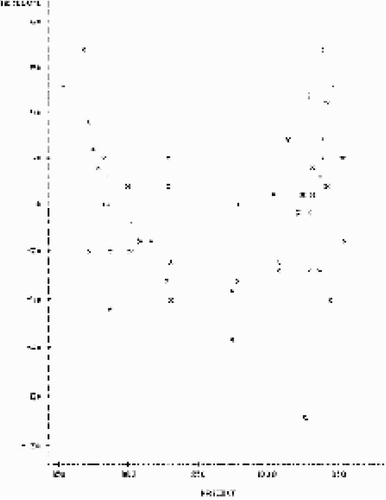
7 Although some guidance from the instructor is to be expected, students should be encouraged to examine the data thoroughly before attempting to resolve the spending/performance paradox. They should note the general properties of each of the variables, including their range and any obvious outliers. They may also wish to rank the states in ascending or descending order based on their public school expenditures and/or SAT performance. Do the same states appear at or near the top of each list? Why or why not? To answer that question easily, students should be encouraged the view the relationship between spending and performance visually in a scatterplot (Figure 1).

Figure 1. Current Per-Pupil Expenditure by Average SAT Score

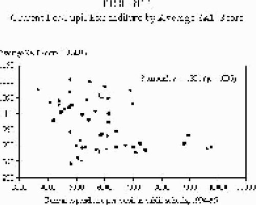
8 As the scatterplot demonstrates, the relationship between expenditures and performance appears to be negative — that is, the states that score highest on the SAT are the states that, on average, spend less money per student. For example, high spending states such as New Jersey, New York, Alaska, and Connecticut all post aggregate scores well below the national average combined score of 966.

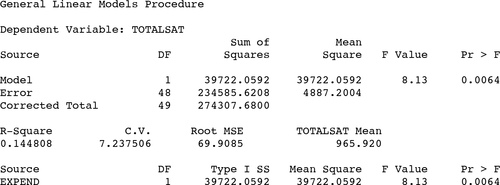
9 These results can be further summarized in a simple bivariate regression. As the model shown in Table 1 suggests, every $1,000 increase in spending per student per year is associated with a decline of nearly 21 points in the average statewide SAT score, an estimate that easily reaches conventional levels of statistical significance (p < .01).

Table 1. SAS Regression Output for Bivariate Regression Model

10 The strength of this relationship might seem puzzling to students at first. After all, it suggests not that money is irrelevant to academic performance, but that spending more on public schools only seems to exacerbate the problem. Or does it? Just as SAT scores vary widely from state to state, so too does the percentage of high school students taking the exam. In fact, participation ranges from a high of 81% in Connecticut to a low of 4% in Utah. That rate of participation is determined, in part, by academic interest in attending college, but also by the preferred standardized test in that region. As Hawkins (1994) points out, the ACT remains a popular alternative to the SAT among college admissions offices in certain parts of the country. In these states, a select group of bright students intent on attending competitive out-of-state schools are more likely to take (and score well on) the SAT.

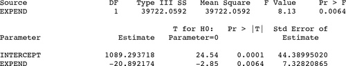
11 The consequence of this may not be immediately apparent to the class, but the issue should lead to a lively discussion. For example, if the very best students in each state self-select themselves into the pool of test-takers, the average score naturally rises. Conversely, in states such as Connecticut, Massachusetts, New York, and New Jersey, where a substantial majority of high school students take the SAT, a less elite population of students contributes to a lower average score. The strength and importance of this relationship can be confirmed with a scatterplot and/or a Pearson’s correlation coefficient (Figure 2).

Figure 2. Average SAT Score by the Percentage of All Eligible Students Taking the Test

12 Does the composition of test-takers influence our original question relating to school expenditures and academic performance? Indeed it does. Without controlling for the percentage of students taking the exam, the correlation between spending and performance was a surprising -.381 (p = .006). However, when a partial correlation is used to provide statistical control for this previously omitted variable, the coefficient reverses to +.391 (p = .000). (For greater detail on the use and calculation of partial correlation coefficients, see Kachigan 1982, pp. 153-155.)

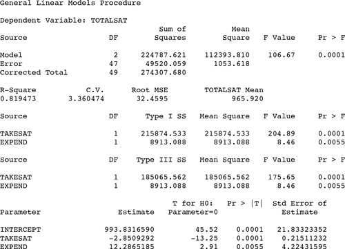
13 A dramatic improvement in model fit can also be seen in a second multiple regression model, shown in Table 2. With a robust R2 and slope coefficients that are both highly statistically significant (p < .01), it is now clear that while the bulk of variation in statewide SAT scores is attributable to the percentage of students taking the exam, increased spending on public education is in fact associated with better academic performance.

Table 2. SAS Regression Output for Multiple Regression Model

14 While the analysis presented up to this point is quite simple to reproduce in the classroom, it should be noted that this dataset is worth exploring further using more sophisticated techniques. For instance, if time and interest permit, students may want to test the importance of school expenditures in a more complex model. Several additional variables are provided for this purpose, including student/teacher ratios and average annual teacher salaries.

15 The dataset also gives an instructor the opportunity to address common hazards in regression analysis. For example, astute students who visually plot the residuals from the second regression model might question an irregular U-shaped pattern that clearly hints at a nonlinearity problem involving the percentage of students taking the SAT (Figure 3). Since an assumption of linearity is key to ordinary least squares regression estimation, students could be instructed on a variety of possible solutions, including the addition of a polynomial term to the equation or a logarithmic transformation (Lewis-Beck 1980). Powell and Steelman (1984, 1996) address this very issue at some length and find that the best-fitting nonlinear regression equation is one that includes both the percentage of test-takers and its square root, a conclusion that could be tested and confirmed in the classroom.

Figure 3. Residual Plot for Multiple Regression Model

5. Conclusion

16 As the debate over public school expenditures rages on, it is clear that simple statistical analyses can mislead pundits, policymakers, and parents alike. The goal of this exercise is to encourage students to be acutely sensitive to these debates and to the way in which statistics are used to inform various political arguments publicized in the news media.

17 Aside from that note of warning, however, what contribution does this dataset make to our understanding of the public school debate? Do the data conclusively “prove” that spending more money on public education produces better results? Hardly, although the case is instructive in many ways. As Hawkins (1994, p. 26) warns, “The question of whether money matters in the public schools is a legitimate research question. In fact, under the right research conditions, it might be possible to answer it. Simple correlations based on aggregated data from the 50 states, however, don’t begin to adequately explain the complexities.” For example, knowing that money matters does not solve the riddle of “when,” and “under what conditions.” Nor does it tell us how that money should be spent in order to produce the biggest bang for the buck. In the end, the strength of this exercise rests not only on what issues are resolved, but also on the importance of those that remain.

6. Getting The Data

18 The file sat.dat.txt contains the raw data. The file sat.txt is a documentation file containing a brief description of the dataset.

Appendix -

Key To Variables in sat.dat.txt

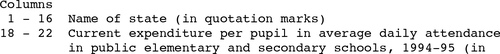
Values are aligned and delimited by blanks. There are no missing values.

References

- Hawkins, J. A. (1994), “Money Matters! But What Difference Does It Make to Schools and Students?” NASSP Bulletin, 78, 19–26.
- Kachigan, S. K. (1982), Multivariate Statistical Analysis: A Conceptual Introduction. New York: Radius Press.
- Lewis-Beck, M. S. (1980), Applied Regression: An Introduction. Newbury Park, CA: Sage Publications.
- National Center for Education Statistics ( 1997), Digest of Education Statistics [ Online], Washington, DC: U.S. Department of Health, Education, and Welfare, Education Division. (http://nces01.ed.gov/pubs/digest97/index.html)
- Powell, B., and L. C. Steelman (1984), “Variations in State SAT Performance: Meaningful or Misleading?” Harvard Educational Review, 389–410.
- Powell, B., and L. C. Steelman (1996), “Bewitched, Bothered and Bewildering: The Use and Misuse of State SAT and ACT Scores,” Harvard Educational Review, 27–59.
- Will, G. F. ( September 12, 1993), “Meaningless Money Factor,” The Washington Post, C7.