Replacing a 'Striped-Box' with the Normal Approximation

Abstract

A simple procedure is presented for obtaining the sample size and acceptance number for a single sample acceptance sampling plan, given the probability of lot acceptance for lots having proportion defective equal to p₁, and the probability of lot rejection for lots having proportion defective equal to p₂. The procedure gives a practical illustration of the use of the normal approximation to the binomial distribution that is appropriate for courses on statistical quality control as well as on introductory statistics.

Keywords:

• Acceptance sampling
• Binomial nomograph
• Single-sampling plan

1. Introduction

1 The most basic acceptance sampling plan considered in courses on statistical quality control can be described as follows. A large lot of items is to be inspected in order to ascertain its quality. A random sample of n items is selected, and D, the number of defectives (or nonconforming items) in the sample is counted. If D exceeds c, the acceptance number, then the lot is rejected. Otherwise, it is accepted. This is the so-called single-sampling plan.

2 Because of the simplicity and practicality of such plans, they are also appropriate for discussion or exercises in introductory courses on statistics, especially those designed for mathematics or statistics majors. They are useful as examples of binomial and hypergeometric models. In addition, the designing of such plans (that is, deciding upon n and c) provides nice nontrivial examples of the use of the normal approximation to the binomial distribution, highlighting the importance of the continuity correction, which is often one of the more difficult topics to motivate in an introductory course. Strangely, the approach taken toward designing such plans described in popular quality control textbooks avoids mention of the normal approximation to the binomial, even if the approximation is described in the ‘statistical background’ chapter. Instead, a ‘black-box’ method based on something called a binomial nomograph is described (see, e.g., Montgomery 1996), and an opportunity to demonstrate the normal approximation in a practical setting is missed.

3 Such plans are usually designed (that is, n and c are chosen) to satisfy the competing interests of the lot producer and the lot consumer. The lot producer would like the probability of lot acceptance (1–α) to be high when the proportion of nonconforming units (p₁) is low. The consumer requires the probability of lot acceptance (β) to be low when the proportion of nonconforming units (p₂) is high. In the quality control textbook by Montgomery (1996, p. 620), it is stated that n and c should be taken to satisfy $$1-\alpha ={\displaystyle \sum _{d=0}^c\left(\frac{n}{d}\right)p_1^d{\left(1-p_1\right)}^{n-d}.}$$(1)

and $$\beta ={\displaystyle \sum _{d=0}^c\left(\frac{n}{d}\right)p_2^d{\left(1-p_2\right)}^{n-d}.}$$(2)

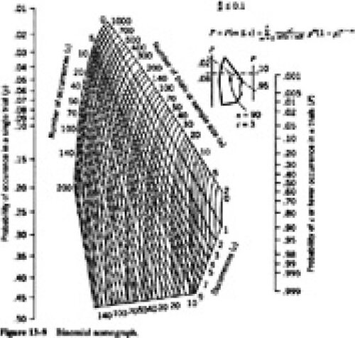
Montgomery goes on to say that the nonlinear equations (1)$$1-\alpha ={\displaystyle \sum _{d=0}^c\left(\frac{n}{d}\right)p_1^d{\left(1-p_1\right)}^{n-d}.}$$(1) and (2)$$\beta ={\displaystyle \sum _{d=0}^c\left(\frac{n}{d}\right)p_2^d{\left(1-p_2\right)}^{n-d}.}$$(2) have no simple, direct solution. A binomial nomograph is then exhibited for use in obtaining solutions to these equations. The nomograph is a nonregular grid for which a relatively simple, but apparently magical, set of rules can be followed to obtain n and c, for given α,β, p₁, and p₂. An equivalently magical procedure is provided by Mitra (1998, p. 438-441), in which case a table of Grubbs (1949) has been used to obtain sampling plans.

Figure 1. A Binomial Nomograph from Montgomery (1996, p. 620) (used with permission).

4 The goal of the present note is to make some remarks about the above equations and procedure and to present an alternative, simpler procedure for designing single-sampling plans. The idea is that the normal approximation to the binomial distribution leads to approximations for n and c, given and . A key motivation is to replace the black-box nature of the above nomograph procedure with a procedure that can be relatively easily understood. Such a procedure could be demonstrated in either an introductory statistics course or in a quality control course.

2. Some Remarks and the Normal Approximation Solution

5 The first thing to observe is that the nonlinear equations will usually not have an integer-valued solution. Thus, the nomograph will not usually provide a true solution, but it will yield an approximate solution. This will be accomplished by choosing the nearest grid point on the nomograph to the real-valued solution that the nomograph provides. One problem with this technique is that the resulting sampling design may sometimes result in probabilities of acceptance that are too low at p₁ and/or too high at p₂. What is really sought is a sampling design that satisfies (or comes close to satisfying) the inequalities $$1-\alpha \le {\displaystyle \sum _{d=0}^c\left(\frac{n}{d}\right)}{p}_1^d{\left(1-p_1\right)}^{n-d}$$(3)

and $$\beta \ge {\displaystyle \sum _{d=0}^c\left(\frac{n}{d}\right)}{p}_2^d{\left(1-p_2\right)}^{n-d}.$$(4)

Usually, one would want to use the smallest value of n satisfying both inequalities. Using the normal approximation to the binomial distribution with the continuity correction, we have $$P\left(D\le c\right)=P\left(D<c+0.5\right)\doteq P\left(Z<\frac{c+.5-np}{\sqrt{np(1-p)}}\right)$$(5)

where Z is a standard normal random variable. Thus, inequality (3) implies $$\frac{c+.5-n{p}_1}{\sqrt{n{p}_1(1-p_1)}}\ge z_{\alpha }$$(6)

where $P(Z>z_{\alpha })=\alpha$, and inequality (4) implies $$\frac{c+.5-n{p}_2}{\sqrt{n{p}_2(1-p_2)}}\le -z_{\beta }.$$(7)

Thus, $$c\ge z_{\alpha }\sqrt{n{p}_1\left(1-p_1\right)}+n{p}_1-.5$$(8)

and $$c\le -z_{\beta }\sqrt{n{p}_2\left(1-p_2\right)}+n{p}_2-\mathrm{.5.}$$(9)

A quadratic inequality in $\sqrt{n}$ can then be obtained by subtracting the first inequality from the second. The relevant solution satisfies $$\sqrt{n}\ge \frac{z_{\alpha }\sqrt{p_1\left(1-p_1\right)}+z_{\beta }\sqrt{p_2\left(1-p_2\right)}}{p_2-p_1}.$$(10)

One possible value of n to try is the smallest integer satisfying the above inequality. The value of c may then be chosen as the smallest integer satisfying (8). However, the previously chosen value of n may not satisfy (9) for this particular value of c, so the value of n may need to be revised accordingly. This time, (9) may be viewed as a quadratic inequality in $\sqrt{n}$, and the relevant solution set is given by $$\sqrt{n}\ge \frac{z_{\beta }\sqrt{p_2(1-p_2)}+\sqrt{z_{\beta }^2{p}_2\left(1-p_2\right)+4(c+.5)p_2}}{2p_2}$$(11)

The value of n should then be taken as the smallest integer satisfying (11). In some circumstances, one may wish to revise c, using the newly revised value of n and inequality (8), but this is usually not necessary.

6 Table1 gives an indication of the quality of the sampling plans obtained using the normal approximation (with continuity correction) for some typical situations. The nominal values of α,β, and p₁ are fixed at .05, .1, and .01, respectively. The table provides the sampling plans for the tabulated values of p2, and also gives the true binomial probabilities $\alpha =P\left(D>c\right)$ (at p₁) and $\beta =P\left(D\le c\right)$ (at p₂). These are listed in the fourth and fifth columns, respectively.

Table 1. Some Continuity Corrected Single-Sampling Plans for Various Values of p₂, With p₁ = 0.01, α= 0.05 (Nominal), and β= 0.1 (Nominal), Together With Actual Probabilities of Lot Rejection (at p₁) and Acceptance (at p₂)

p2	n	c	α	β	error in α	error in β
0.020	1184	17	0.0561	0.0952	0.122	0
0.025	620	10	0.0505	0.0933	0.011	0
0.030	395	7	0.0473	0.0929	0	0
0.035	268	5	0.0542	0.0905	0.084	0
0.040	202	4	0.0536	0.0906	0.071	0
0.045	179	4	0.0349	0.0914	0	0
0.050	135	3	0.0474	0.0901	0	0
0.060	90	2	0.0619	0.0880	0.239	0
0.070	77	2	0.0424	0.0875	0	0
0.080	67	2	0.0298	0.0882	0	0
0.090	60	2	0.0224	0.0846	0	0
0.100	40	1	0.0607	0.0805	0.215	0
0.120	33	1	0.0430	0.0810	0	0
0.150	26	1	0.0277	0.0817	0	0

NOTE: The relative error in the constraints (3) and (4) is indicated in the last two columns.

7 It should be noted that, because the normal approximation is used, the required inequalities are sometimes mildly violated, especially (3); however, the violations are usually no worse than those for the Grubbs’ table or the nomograph. The sixth and seventh columns of Table 1 indicates the relative size of these errors. That is, $$errorin\alpha =\max \left(\frac{0.05-\alpha }{0.05},0\right)$$

and $$errorin\beta =\max \left(\frac{\beta -0.1}{0.1},0\right)$$

8 The method is surprisingly accurate even for cases where n turns out to have a small value. This is consistent with observations made by Kupper and Hafner (1989) about finding sample sizes for hypothesis tests when both test size and power at a particular alternative are specified.

3. Discussion

9 In practice, one could check $P\left(D\le c\right)$ for both values of p to ensure that the sampling plan is satisfactory. If it is not, one could experiment with slightly larger values of n (together with the corresponding c values) to obtain plans that conform more closely to the nominal values of α and β.

10 It is also possible to try to correct the approximation using Cornish-Fisher expansions (e.g., Hall 1992). For example, one can show that $$c\ge n{p}_1-.5+z_{\alpha }\sqrt{n{p}_1(1-p_1)}-\left(1-2p_1\right)(1-z_{\alpha }^2)/6+O(n^{-1/2})$$(12)

and $$c\le n{p}_1-.5+z_{\beta }\sqrt{n{p}_2(1-p_2)}-\left(1-2p_2\right)(1-z_{\beta }^2)/6+O(n^{-1/2}).$$(13)

Then, a sampling plan can be obtained by solving another quadratic inequality for $\sqrt{n}$. The resulting plans obey inequalities (3) and (4) more often than the uncorrected plans. Table 2 lists the corrected plans that correspond to the ones in Table 1, together with the actual probabilities of rejection at p₁ and acceptance at p₂. Although not listed in the table, there are some plans found by this procedure that violate inequality (3).

Table 2. Cornish-Fisher Corrected Single-Sampling Plans for Various Values of p₂, With p₁ = 0.01,α= 0.05 (Nominal), and β= 0.1 (Nominal), Together With Actual Probabilities of Lot Rejection (at p₁) and Acceptance (at p₂)

p2	n	c	α	β	error in α	error in β
0.020	1236	18	0.0466	0.0989	0	0
0.025	615	10	0.0483	0.0985	0	0
0.030	391	7	0.0451	0.0985	0	0
0.035	300	6	0.0328	0.0976	0	0
0.040	231	5	0.0298	0.0972	0	0
0.045	177	4	0.0335	0.0964	0	0
0.050	133	3	0.0453	0.0961	0	0
0.060	110	3	0.0250	0.0980	0	0
0.070	75	2	0.0397	0.0968	0	0
0.080	66	2	0.0287	0.0935	0	0
0.090	58	2	0.0205	0.0965	0	0
0.100	52	2	0.0154	0.0966	0	0
0.120	43	2	0.0092	0.0970	0	0
0.150	25	1	0.0258	0.0931	0	0

NOTE: The relative error in the constraints (3) and (4) is indicated in the last two columns.

11 One might argue that when using the Cornish-Fisher correction, the simplicity and directness of the method are sacrificed. For most practical purposes, the normal approximation is probably adequate, and it is certainly easier for an undergraduate student to understand. On the other hand, it might not hurt for a senior undergraduate to see that there are relatively simple ways to improve on the normal approximation.

12 The continuity correction itself seems to be necessary in order to provide accurate results. If the correction is ignored, the above inequalities are violated fairly often, and sometimes by a substantial margin, as can be seen from Table 3. That table corresponds exactly to Table 1, except that $$c\ge z_{\alpha }\sqrt{n{p}_1\left(1-p_1\right)}+n{p}_1$$

is used in place of (8) and $$\sqrt{n}\ge \frac{z_{\beta }\sqrt{p_2(1-p_2)}+\sqrt{z_{\beta }^2{p}_2\left(1-p_2\right)+4(c)p_2}}{2p_2}$$

is used in place of (11). Inequality (10) is still used to obtain the initial estimate of n.

Table 3. Uncorrected Single-Sampling Plans for Various Values of p₂, With p₁ = 0.01, α= 0.05 (Nominal), and β= 0.1 (Nominal), Together With Actual Probabilities of Lot Rejection (at p₁) and Acceptance (at p₂)

p2	n	c	α	β	error in α	error in β
0.020	1213	18	0.0400	0.115	0	0.155
0.025	596	10	0.0401	0.120	0	0.203
0.030	375	7	0.0368	0.123	0	0.240
0.035	286	6	0.0262	0.125	0	0.251
0.040	218	5	0.0233	0.128	0	0.286
0.045	165	4	0.0258	0.131	0	0.317
0.050	148	4	0.0170	0.132	0	0.329
0.060	101	3	0.0189	0.137	0	0.378
0.070	87	3	0.0115	0.133	0	0.339
0.080	59	2	0.0214	0.139	0	0.392
0.090	52	2	0.0153	0.141	0	0.417
0.100	47	2	0.0116	0.138	0	0.383
0.120	39	2	0.0069	0.137	0	0.374
0.150	21	1	0.0185	0.155	0	0.550

NOTE: The relative error in the constraints (3) and (4) is indicated in the last two columns.

13 It should be noted that the nomograph is unable to provide sampling plans outside a certain range. For example, if α= .001, β= .1, p₁ = .01, and p₂ = .02, then the nomograph cannot be used to obtain a plan, but the normal approximation method gives the sampling plan: n = 2416 and c = 39 and $$P\left(D\le c\right)=0.0018ifp=.01$$

and $$P(D\le c)=0.097ifp=\mathrm{.02.}$$

Also, the nomograph will not yield any sampling plans when p < .01. The Grubbs’ table will not provide any sampling plans where c exceeds 15. The normal approximation is much more widely applicable.

14 Finally, there is the important pedagogical value of the above approach. Not only is this a relatively simple way to replace a black-box (or striped-box) solution, but it is also a useful application of the normal approximation to the binomial distribution.

Acknowledgments

The helpful comments and suggestions of three anonymous referees have led to a substantial improvement in the paper and are gratefully acknowledged. This work was supported by a research grant from the Natural Sciences and Engineering Research Council of Canada (NSERC) and was completed during a visit to the Centre for Mathematics and Its Applications at the Australian National University in Canberra, Australia.

References

- Grubbs, F. E. (1949), “On Designing Single Sampling Plans,” Annals of Mathematical Statistics, 20, 256.
- Hall, P. (1992), The Bootstrap and Edgeworth Expansion, New York: Springer-Verlag.
- Kupper, L. L., and Hafner, K. B. (1989), ”How Appropriate Are Popular Sample Size Formulas?” The American Statistician, 43, 101–105.
- Mitra, A. (1998), Fundamentals of Quality Control and Improvement (2nd ed.), Upper Saddle River, New Jersey:Prentice Hall.
- Montgomery, D. C. (1996), Introduction to Statistical Quality Control (3rd ed.), New York: Wiley.