Teaching Prediction Intervals

Abstract

Teaching prediction intervals to introductory audiences presents unique opportunities. In this article I present a strategy for involving students in the development of a nonparametric prediction interval. Properties of the resulting procedure, as well as related concepts and similar procedures that appear throughout statistics, may be illustrated and investigated within the concrete context of the data. I suggest a generalization of the usual normal theory prediction interval. This generalization, in tandem with the nonparametric method, results in an approach to prediction that may be systematically deployed throughout a course in introductory statistics.

Keywords:

• Confidence interval
• Descriptive statistic
• Error reduction
• Normal distribution
• Percentile

1. Introduction

1 The prediction interval generally occupies a rather small niche in introductory statistics courses. This is unfortunate because there are meaningful applications for prediction intervals, as well as sound pedagogical reasons for covering the topic thoroughly. Recent articles by Whitmore (1986), Scheuer (1990), and Vardeman (1992) argue in favor of placing more emphasis on the prediction interval. In this article I present strategies for teaching the prediction interval effectively, efficiently, and comprehensively. My exposition largely targets the non-calculus-based introductory applied statistics course; the material is easily adapted for other audiences.

2 One especially attractive opportunity afforded by teaching prediction intervals is that with minimal guidance— and no formal background in probability—students can develop the nonparametric prediction interval (treated in Section 3). The development is visual in nature; the method is applied without resorting to a formula.

3 Prediction intervals are generally treated as inferential methods, but there are good reasons for integrating the nonparametric prediction interval into coverage of descriptive statistics. Students readily agree that a procedure that predicts future observations with a given level of confidence ought to predict the data on hand at approximately that level (the slight difference is clarified by the visual device used to develop the nonparametric prediction interval). Consequently, a prediction interval, when plotted to accompany graphically displayed data, is validated by the data. Further, percentiles, an important descriptive measure, may be associated with prediction intervals. Presenting the two together yields a consistent approach to forming statistical intervals.

4 The nonparametric prediction interval also offers advantages when discussing inferential methods. This interval introduces the idea of inference based on order without requiring combinatorics, nor a parameter to be estimated. It shares properties with other statistical intervals, and some generalizations about statistical intervals are illustrated quickly, and concretely, via appeal to the nonparametric prediction interval. On the other hand, obtaining a prediction interval in conjunction with a confidence interval (CI) disavows a number of students of a misconception about CIs, namely that “C% of the data lies between L and U.”

5 Applications for prediction intervals are found in a number of settings, including business and quality control; see, for instance, Patel (1989, p. 2396), Scheaffer and McClave (1990, p. 292), Hahn and Meeker (1991, p. 31), Vardeman (1994, p. 347), and Neter, Kutner, Nachtsheim, and Wasserman (1996, pp. 65-66). In contrast to textbook coverage of prediction intervals, which is usually restricted to regression situations (in the limited sense of regression as curve-fitting), these applications exist for the variety of standard models covered in introductory courses. Prediction intervals are obtained in identical fashion for each of these models, reinforcing the perspective of a symmetric approach to a variety of situations.

6 This article focuses on strategies for teaching prediction intervals, and on ways to use prediction intervals to introduce and illustrate other important statistical tools and concepts in a fairly benign setting. The material in this article was developed to serve an audience that is not mathematically sophisticated, is prone to choose blind computation over reflection and interpretation, and is quantitatively timid (and consequently often intimidated). My students have average algebra skills; a sizable minority have taken a single semester of calculus—generally business calculus. They need considerable guidance developing an appreciation for the systematic fashion in which statistical methods are deployed. They need simple, concrete examples that demonstrate the nature of inferential statements. My premise in designing these materials was to illustrate statistical concepts, and relationships among them, in direct reference to observed data, and to develop techniques that are used the same way in a variety of models.

7 In what follows I discuss methods that succeed in my classroom. They succeed in part by simply allowing students to take some small amount of ownership in the theory; in part by taking advantage of prediction’s direct association with the data, as a consequence making concrete the illustration of more sophisticated concepts; and in part by developing a systematic framework for constructing statistical intervals—one that may be applied in a variety of situations. My aim is to convince you that a comprehensive treatment of prediction intervals addresses fundamental statistical issues—issues that may be introduced early in an introductory statistics course, then revisited, extended, elaborated upon, and contrasted with other statistical tools.

1.1 Organization

8 Formal definitions are established in Section 2. In Section 3, I introduce the one-sample nonparametric prediction interval. The relationship between this prediction interval and percentiles is pursued. An application for this prediction interval in a descriptive treatment of simple linear regression is also presented. In Section 4, I discuss a generalization of the normal theory prediction interval covered in many textbooks. In Section 5, the nonparametric prediction interval and the normal theory prediction interval are compared. Illustrations throughout are in terms of two-sided intervals; treatment of one-sided intervals is analogous (students will likely suggest one-sided procedures when given the chance to work with the nonparametric prediction interval). Details on the data-generating activity mentioned in Section 3.1, Minitab macros for obtaining prediction intervals and percentiles, and some remarks on textbook treatments of prediction, are included in Appendices A, B, and C, respectively.

9 Different courses and different instructors address topics in any number of sequences. In my courses I typically cover the material in this article as follows.

•	The nonparametric prediction interval of Section 3 very near the onset of the course, as part of a unit on descriptive and graphical methods. Prediction intervals make a first appearance just prior to percentiles.
•	The probability prediction interval of Section 2.1 during a subsequent (and short) unit on probability.
•	A substantial portion of the remaining course time is allocated to coverage of both descriptive and inferential tools for a variety of models involving a quantitative response (one-sample, multi-sample, and regression settings). Because properties and interpretation of prediction intervals are most easily demonstrated with the one-sample nonparametric prediction interval of Section 3.1, I review the method before moving on to the normal theory prediction interval. At this point I explicitly present the formal definition of a prediction interval stated by (2) of Section 2.2. I cover the normal theory prediction interval of Section 4 in each of the standard models, positioning the nonparametric prediction interval as an alternative for situations in which the normal theory prediction interval is inappropriate.

I do not explicitly treat the finer points on robustness issues stated in Sections 3.4 and 4.2. However, proper use and interpretation of the prediction interval is a semester-long goal. My coverage of prediction takes very little time out of an already busy semester, while allowing for efficiencies along the way.

1.2 Notation

10 Throughout this article, I’ve attempted to distinguish formal notation as it is used to express generalized results. For the most part this is not the notation I use with students. They are expected instead to use the ideas presented in class, and to visualize situations to motivate solutions and interpretations, as in Figures 1, 2, and 3. I do make use of notation utilized in an accompanying textbook (for, say, percentiles), with but one exception: for normal data my students learn (6) in conjunction with (7) in place of expressions such as (5).

2. Definitions

11 Assume that a continuous response variable Y, perhaps a function of explanatory variables, is randomly sampled from a population.

2.1 Probability Prediction Intervals

12 For $\alpha$ between 0 and 1 (an error rate), let y_L and y_U denote the ($\alpha$/2) × 100th and (1 - $\alpha$/2) × 100th percentiles, respectively, of the population distribution for Y. Then a (1 - $\alpha$) × 100% probability prediction interval (PPI) for the outcome Y is given by (y_L, y_U). A population distribution is often conveniently expressed in mathematical terms by a density function. The most commonly treated of these mathematical idealizations is the normal distribution. For univariate normal data, mean $\mu$ and standard deviation $\sigma$, the PPI for a randomly selected observation is $$\left(\mu -z_{\alpha /2}\sigma ,\mu +z_{\alpha /2}\sigma \right)$$(1)

Analogous statements exist for distributions other than the normal. The probability is (1 - $\alpha$) that a randomly selected observation drawn from the specified population will fall within the bounds of such an interval; equivalently, (1 - $\alpha$) × 100% of the population falls within these bounds. Treating prediction in this context provides practice at obtaining appropriate percentiles—a task that is often required when constructing confidence intervals and computing observed significance levels.

2.2 Statistical Prediction Intervals

13 In applications, a complete specification for the population distribution is often unknown. Assume a random sample, Y_i, i = 1,…, n, is to be drawn; from this sample values ${\widehat{Y}}_L$ and ${\widehat{Y}}_U$ are to be obtained. If, for a subsequent randomly sampled observation Y, $$P\left[{\widehat{Y}}_L<Y<{\widehat{Y}}_U\right]=1-\alpha ,$$(2)

then the observed interval $\left(\widehat{y}L-\widehat{y}U\right)$ is a (1 - $\alpha$) × 100% statistical prediction interval (hereafter, simply prediction interval, or PI) for Y (Patel 1989). For standard linear models where residuals are normally distributed with unknown common variance, an appropriate PI is formed by (6) and (7) of Section 4. A nonparametric alternative for the one-sample model is given by (3) of Section 3. Methods for other parameterizations are catalogued in Patel (1989) and Hahn and Meeker (1991).

14 Note that the specified probability of (1 - $\alpha$) is a priori of observing the sample. The (conditional) probability that Y falls within the observed bounds of the interval, $P\left[\widehat{y}L<Y<\widehat{y}U\right]$, is generally unknown. In Section 3,

I describe a short, simple demonstration that exposes this distinction, the nature of which is also at the heart of a conceptual understanding of confidence intervals.

3. The Nonparametric Prediction Interval

15 I teach the prediction interval quite early in my courses, weaving it into a discussion of descriptive and graphical methods as early as the first week of classes. By asking the right questions, I provide a touch of direction—my students then rather quickly produce the nonparametric PI. Development of this PI leads naturally to a definition of percentiles. I also apply this PI in an activity that demonstrates the utility of residual analysis when quantifying the effects of adjusting for a predictor variable in simple linear regression.

3.1 One-Sample Prediction Intervals

16 Developing a prediction procedure that satisfies (2) is straightforward and requires of students only minimal intuition about probability. A simple example that I use with classes suffices as illustration.

17 Each student is assigned to monitor one of a population of manufactured components in stock. (I use matches as surrogates for these components; each student has measured the amount of time it takes a match to burn out. See Appendix A for details.) A random allocation has put 19 of these components to use. We desire to warrant the next (20th) component on the basis of the failure times of the first 19 components. (Another application uses the first 19 observations to form control limits.) Our job is to predict, on the basis of 19 randomly sampled observations, a subsequent 20th observation.

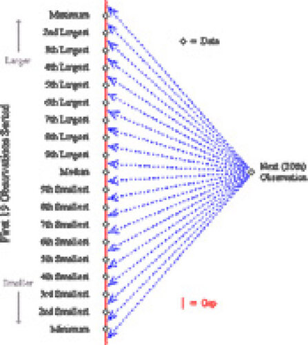
18 Without explicitly stating what I mean by it, the class is made aware that a “confidence figure” will accompany the prediction. I prompt: What is the probability the 20th value is the smallest? second smallest? and so on. Students readily respond that the 20th observation is equally likely (probability 1/20) to occupy any of positions 1 through 20 in the ordered list of all 20 observations. I then show them the diagram displayed in Figure 1—directing their attention to the 20 gaps formed by the first 19 observations. This suggests that 1/20 is the probability that the 20th observation falls in any particular gap formed by the ordered sample of 19 observations. Students quickly point out that the minimum and maximum form 90% prediction bounds, as the subsequent observation has 1/20 probability of falling outside either bound. In a similar fashion, the second smallest and second largest values bound an 80% PI, and so forth. Students are quick to suggest alternate solutions, some of which lead naturally to the development of one-sided intervals.

Figure 1. Gaps Between Consecutive Ordered Observations. This diagram draws attention to the gaps between consecutive ordered observations in a sample of size 19. The next observation is equally likely to occupy each of these 20 gaps.

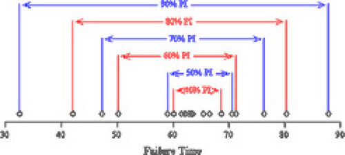
19 The demonstration proceeds: 19 students, from a class of 75, are randomly sampled; the failure times of 19 components are reported in Table 1. The 90% PI, bounded by the extreme observations, is (32.56, 87.87), the

80% PI is (42.02, 80.37), and so on. The data and selected PIs are graphically depicted in Figure 2. Already, without resorting to any notation nor a formula, the relationship (common to all statistical intervals) between interval width and confidence level is established.

Table 1. Failure Times of 19 Randomly Sampled Components

Failure time (sorted)
32.56	42.02	47.26	50.25	59.03	60.17	61.56	62.16	62.84	63.29
63.52	65.52	66.54	68.71	70.60	71.27	76.33	80.37	87.87

Figure 2. Dotplot of Failure Times. A dotplot of the failure time data of Table 1 is displayed. One-sample nonparametric prediction intervals are shown for a variety of levels.

20 Formally, given a random sample of size n and subsequent observation Y, with Y_(i) denoting the ith order statistic among the initial n observations, and j some index between 1 and [n/2],

$$P\left[Y_{\left(j\right)}<Y<Y_{\left(n+1-j\right)}\right]=1-\frac{2j}{n+1}$$.

Consequently, $$\left(y_{(j),}{y}_{(n+1-j)}\right)isa\left(1-\alpha \right)\times 100\%PI,where\alpha =\frac{2j}{n+1}.$$(3)

(Wilks 1941). (My students are required to visualize and think through the argument rather than apply this sort of notation.)

21 We continue with the demonstration, using the 90% interval. A randomly selected 20th component is put to work and the failure time observed: It either does or does not fall within the observed bounds of the interval. Retrenching, I survey the failure times of each of the remaining 56 components (originally unsampled): 52, or 92.86%, have failure time between the observed bounds of the 90% PI. The confidence level of 90% is not the probability a subsequent value falls between the observed extremes—90% is instead a property of the procedure. (The point is made with but a single unsampled unit.) This is also evident from the relative sizes of the observed gaps. After plotting the 19 sampled values, students agree that the gap of 2.99 between the third and fourth smallest values is less likely to include a subsequent value than is the gap of 8.78 between the fourth and fifth smallest values. The argument they’ve bought into (20 gaps of 1/20 probability each) works only on average, not in particular cases.

22 An interpretation is reinforced by repeating the demonstration.

•	On average the observed bounds have .90 probability of including the next observation.
•	90% of the time the entire procedure is implemented, the subsequent 20th observation falls within the bounds obtained from the first 19 observations.

If nothing else, students are now convinced that results of even the simplest statistical procedures must be interpreted carefully. (As numerous opportunities arise later, I prefer not to dwell too long on such conceptual issues while still covering descriptive methods.)

23 It is worthwhile to demonstrate how matters progress differently when the entire population is specified in advance. (Because students obtain data prior to class, and in my presence, I have the luxury of precomputing PPIs.) Here a PPI is obtained—the bounds are not subject to sampling variability. However, knowledge of PPI bounds implies a complete specification for the population distribution—an unrealistic assumption to make in many situations.

24 The demonstration itself provides ample practice for most students. I do assign a few exercises to be done by hand; I supply sorted data and call for exactly attainable levels. I touch on the idea of being conservative when levels are not so convenient and briefly mention interpolation. Beyond this it is assumed that software will do the computing. (A Minitab macro for obtaining one-sample PIs is provided in Appendix B.)

25 The application of this PI as a formal inference requires randomly sampled data. In any case, however, this PI does form an (approximate) statement about the observed data, as approximately (1 - $\alpha$) × 100% of the sample data lies within the bounds. I believe that this is a relevant observation to make with students—a procedure that aims to predict a future value at level (1 - $\alpha$) × 100% ought to predict the observed data at at least approximately this level. (The prediction perspective clarifies the slight disparity—we predict the gaps. However, there is one gap per observation, with but a single gap left over. As a result, including gaps is roughly equivalent to including observations.) Ignoring the finer points then, we have connections between the PI, the related descriptive measure of percentile (discussed in the next section), the graphical device(s) used to display the data, and, in some cases, the empirical rule.

3.2 An Associated Topic: Percentiles

26 The treatment of PIs presented in this article results in no small part from my desire to create more uses for percentiles. Percentiles are fundamental descriptive measures that I expect students to master.

27 Informally, prediction bounds may be viewed as estimates of the population percentiles that form PPI bounds (Vardeman 1994, p. 339, and McClave, Dietrich, and Sincich 1997, p. 516, implicitly suggest this relationship). Defining percentiles appropriately results in a unity across statistical intervals (PPIs, PIs, and many CIs): use—at least in part—percentiles to obtain interval bounds.

28 Return to the example cited above, where the sample size is 19. Again use the 20 gaps to divide the whole into parts. In case of a random sample, since on average 5% of the unsampled observations lie below the minimum sample value, it is reasonable to take the minimum to be the (sample) 5th percentile. To generalize this result, formally define sample percentiles as follows (Gumbel 1939, Weibull 1939). $$Y_{(j),}the{j}^{th}orderstatistic,isthe\frac{j}{n+1}\times {100}^{th}percentile.$$(4)

(A Minitab macro for obtaining these percentiles is provided in Appendix B.)

29 Appealing to the visual devices shown in Figures 1 and 2, students readily associate the bounds of PIs with appropriate percentiles. For example, to obtain a 50% (two-sided) PI, use as bounds the 25th and 75th percentiles. Having discovered this, we quickly reverse direction: from this point forward appropriate percentiles are used to form both one- and two-sided interval bounds.

30 Other definitions exist for sample percentiles— Hyndman and Fan (1996) discuss a number used in various statistical software packages. Using (4) in particular allows for a rigorous association between percentiles and prediction bounds (the rigor pleases me; I’m not certain it matters much to my students). When relying on software that does not make use of (4), PIs constructed from percentiles do not exactly satisfy (2).

3.3 Applying Prediction Intervals in Simple Linear Regression

31 It is now common for a descriptive treatment of simple linear regression to appear early in an introductory statistics course. In treating the situation, I find it useful to apply the nonparametric PI described above. (This is not the familiar version of the PI. Further, the procedure I describe here satisfies (2) only approximately.) I developed the exercise demonstrated below in order to make constructive use of residuals in exposing the fundamental utility of regression: account for variables that affect the response, thereby reducing error and increasing precision in estimating the response.

32 I illustrate with an example. Consider predicting average daily electrical consumption Y, in kilowatt hours per day, given size of residence x, in square feet (data from Graybill, Iyer, and Burdick 1998, pp. 256-257). Appropriate plots are shown in Figure 3. I ask: Given a residence of 1920 square feet, how do we go about forming a 50% PI for the average daily electrical consumption at that residence? Again students take part in developing a method of solution. To begin, I suggest they obtain a 50% PI for electrical consumption—ignoring for the time being residence size. We agree that adjusting our prediction for residence size will improve predictive accuracy. The discussion centers how to achieve this; students have fairly good ideas—typically identifying ends rather than means. It becomes clear that some new tactics are required. We proceed in a fashion that is central to statistical practice: isolate residual from fit. (Statistical software handles the computationally intensive tasks described below.)

1.	Produce a scatterplot. Identify the association as a linear one; check for outliers and leverage values.
2.	Obtain and plot a fitted line (a resistant fit suffices). Here I’ve used the least squares line. At this point, hard copies are distributed; students augment the plot by hand.
3.	Make certain that the equation and plotted line agree by computing the fit at 1920,-13.577 + .033085 × 1920 = 49.943, marking it on the plot. Agree that this value makes a good anchor for our interval.
4.	Obtain the residuals. Make certain we understand what the residuals represent graphically— validating for a few cases that DATA = FIT + RESIDUAL. Produce residual plots.
5.	Obtain appropriate percentiles of the residual distribution. For a 50% PI we need the first and third quartiles; they are -3.066 and 3.755, respectively.
6.	Apply percentiles of the residuals to the fit to form the PI: the lower bound is 49.943 + (-3.066) = 46.877; the upper bound is 49.943 + 3.755 = 53.698. The PI for energy consumption at a residence of 1920 square feet is (46.9 kwh/d, 53.7 kwh/d).
7.	Mark this interval with a vertical bar on the plot.
8.	Repeat steps 3, 6, and 7 for a variety of residence sizes ranging from 1500 to 2400 square feet (this task is distributed among students).
9.	A number of PIs are now plotted as vertical bars over a variety of explanatory levels. Connect the tops (bottoms) of these vertical bars to obtain an upper (lower) prediction limit line. The resulting lines form an (approximate) prediction band.
10.	A confirmatory count reveals that, as it should be, approximately 50% of the observations lie within this band.

In this example the resulting prediction band is nearly coincident with that obtained by the traditional method given by (5) in Section 4.

Figure 3. Applying the Nonparametric PI in Simple Linear Regression. A scatterplot of energy consumption versus size of residence for 40 residences is displayed. The least squares fit and boxplots for both energy consumption (univariate) and the residuals are shown. A one-sample nonparametric 50% PI for the residuals is bounded by the first and third quartiles. This interval is then applied to the fitted line to obtain a prediction band. 50% of the observations lie within this band.

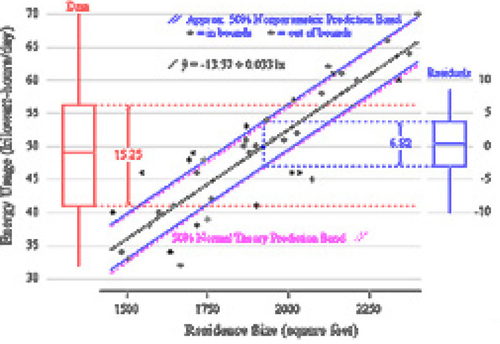
33 Regression is motivated as a reduction of error technique. To illustrate this, I make use of a summary statistic analogous to the coefficient of determination r2 and derived entirely from prediction statements. Continuing with the example, the 50% PI for consumption unadjusted for residence size is (41.00, 56.25), with width 56.25 - 41.00 = 15.25. Next obtain the width of the 50% PI for the residuals: 3.755 - (-3.066) = 6.821. The ratio of these widths, 6.821/15.25 = 0.447, is the fraction of original PI width for estimating energy usage that remains after fitting the line—after adjusting for size of residence. Over half of the prediction error in electricity consumption is accounted for by residence size. (Denote by w this ratio of PI widths. For bivariate normal data and a least squares fit, w and r2 are related: $$\left(1-w^2\right)/r^2\underrightarrow{p}1.$$ In the example, 1 - w2 = 0.800 and r2 = 0.764.)

34 This exercise forces students to make use of a number of important definitions and techniques: fitting a line, obtaining and examining residuals, and finding appropriate percentiles. Both question and solution are addressed by the graphical device.

Question:

[The scatterplot is produced …] A 50% PI should predict approximately 50% of the observed data. What must be done to accomplish this?

Solution:

[The bounds are plotted and …] approximately 50% of the observations fall within the band.

(This sort of motivation/validation is not possible with confidence bounds.) My students find this exercise satisfactory; it builds on previously defined concepts in support of new ideas—in particular residuals—and does so in a straightforward fashion. The results please them and agree with their a priori conjectures.

3.4 Robustness

35 The one-sample nonparametric PI requires only a random sample of observations from a continuous-valued population. As the demonstration of Section 3.1 illustrates, the procedure may be used when randomly sampling without replacement from a finite population—provided there are no ties. In practice there may be ties; generalizations to such situations are possible, but in my view are not worth detailing to an introductory audience. As with other inferential procedures, this PI is not robust against a violation of the assumption of randomly sampled data.

36 The procedure I describe in Section 3.3 does not produce an exact PI. In the general linear model, suppose residual distributions are identical across treatment levels. Forming a nonparametric PI with the pooled residuals, then applying the resulting interval to estimated treatment means (fits) to form PIs at specific treatment levels, does not exactly satisfy the definition of a PI given by (2) —it does so only approximately for large sample sizes, because sampling variability in the estimated means is not accounted for. The normal theory PI is an alternative —provided residual structure is normal. More generally, “…the theory for statistical prediction intervals is complicated” (Hahn and Meeker 1991, p. 242). The definition is exactly satisfied in multi-sample situations provided one does not pool, and forms instead a PI at a given treatment level using the one-sample method with only the data at that level. Such an attack is robust against any violation of the identical distributions across treatment levels assumption. (I find the regression application illustrated above far more useful and do not treat analysis of variance in a similar fashion.)

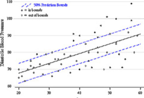
37 In regression applications, it is instructive to demonstrate how the procedure fails in cases of nonconstant variance. To illustrate, consider the data displayed in Figure 4 (data from Neter et al. 1996, p. 407). Systolic blood pressure of healthy women is regressed on age. The 50% prediction band constructed using the method of the Section 3.3 contains—by definition—(approximately) 50% of the data. Yet students who have seen the band plotted on a scatterplot will argue against using the intervals— particularly if it is emphasized that the objective is a procedure that achieves 50% confidence at each age. In short: Don’t use the method to predict unless appropriate assumptions are satisfied. A good lesson!

Figure 4. The PI Fails when Variance is Not Constant. A scatterplot of systolic blood pressure versus age, for healthy women, is displayed. The nonparametric PI is applied with the residuals to obtain a 50% prediction band. Because of nonconstant error variance, the band fails to predict at the 50% level for all ages.

4. Normal Theory Prediction Intervals

38 In the classical model for simple linear regression, the appropriate PI for a future value Y, given explanatory level $x^{\ast }$, is $$\widehat{y}\pm t_{\alpha /2^s}\sqrt{1+\frac{1}{n}+\frac{{\left(x^{\ast }-\overline{x}\right)}^2}{{\displaystyle {\sum }_{i=1}^n{\left(x_i-\overline{x}\right)}^2}},}$$(5)

where s2 is the estimated residual variance. This PI should be computed by software. If a formula is presented, it ought to be one that resorts to minimal notation while still capturing the essence of the method and providing insight into the result. It is also desirable that the procedure be easily generalized to a variety of models, in much the same way as are confidence interval and significance testing procedures.

39 In this section, I suggest a simple, interpretable, alternative formulation for normal theory PIs such as (5). This alternative may be applied in each of the standard models taught in an introductory course— provided the proper assumptions are met. Because the procedure does not share the well-known robustness properties of corresponding confidence interval and significance testing procedures, the section closes with a brief discussion of its robustness.

4.1 A General Expression for Normal Theory Prediction Intervals

40 The standard error of (5) may be recast in friendly and generalizable terms. Assume the classical model where the observed random variables are independent normal with common variance. The expected value of each observation is perhaps a function of explanatory variables. Take $\widehat{y}$ and s2 to be the usual estimates of the mean (expected value) and variance of a subsequent variable Y. Denote by s.e.($\widehat{y}$) the estimated standard deviation (standard error) of the estimate $\widehat{y}$. Define the standard error of prediction for Y by $$s.e.p\left(Y\right)=\sqrt{s^2+s.e{.}^2(\widehat{y})}$$(6)

A PI for Y is then formed by $$\widehat{y}\pm t_{\alpha /2}s.e.p.(Y),$$(7)

using the appropriate error degrees of freedom. (This formulation is merely a re-expression of the normal theory PI that appears in texts. It is well known.)

41 Such a PI is formed out of fundamental quantities: $\widehat{y}$, s.e.($\widehat{y}$), and s are readily obtained using statistical software. When applied in a specific model, (6) yields to algebraic simplification (because s.e.($\widehat{y}$) = cs for some positive constant c), but the simplification really misses the point: This scheme always works the same way.

•	One-sample model. Here $\widehat{y}=\overline{y}$, so $s.e.(\overline{y})=s/\sqrt{n}$. Then (6) may be expressed as

$$s.e.p\left(Y\right)=\sqrt{s^2+\frac{s^2}{n}}=s\sqrt{1+\frac{1}{n}}$$(8)

•

Multi-sample models, assumed equal variance. Samples of sizes nj, j = 1, 2,…, k, are obtained for each of k groups. Assume a prediction is desired for an observation in group j. The estimated mean is $\widehat{y}={\overline{y}}_j$, so $s.e.\left({\widehat{y}}_j\right)=s/\sqrt{n_j}$, where s is the pooled standard deviation.

$$s.e.p\left(Y\right)=\sqrt{s^2+\frac{s^2}{n_j}}=s\sqrt{1+\frac{1}{n_j}}$$

•	Simple linear regression.Since

$$s.e.\left(\widehat{y}\right)=s\sqrt{\frac{1}{n}+\frac{{\left(x^{\ast }-\overline{x}\right)}^2}{{\displaystyle {\sum }_{i=1}^n{\left(x_i-\overline{x}\right)}^2}},}$$(9)

s.e.p.(Y) is as given by (5).

Similar expressions are readily developed for other models.

42 Take, for example, the one-sample normal model: The goal is to use the observed data to make a statement analogous to the PPI given by (1). Adopting the view of PI bounds as estimates of PPI bounds, heuristic justification for the interval formed by applying (6), and then (7), might run as follows.

1.	1. $\sigma$ quantifies unit-to-unit variability. Because it is unknown, replace it with the estimate s.
2.	Estimating $\sigma$ with s entails the use of the t-distribution.
3.	Because the mean $\mu$ is unknown, estimate it with $\overline{y}$.
4.	4.$\overline{y}$ is a variable; the sampling variability in $\overline{y}$ is quantified by s.e. $\left(\overline{y}\right)$.
5.	The formula (6) for s.e.p.(Y) reflects the statistician’s way of combining standard deviations from independent sources (that is, the variances are summed).

43 As with the nonparametric method, this PI is validated by plotting prediction limits along with the data. Implemented when appropriate assumptions are met, approximately (1 - $\alpha$) of the data should fall within the bounds. Comparing prediction bounds to similarly plotted confidence bounds effectively contrasts the two procedures.

44 Few textbooks make use of this approach (I have yet to see it appear in an introductory text of the sort I would consider using). A pleasantly surprising number of my colleagues (all mathematicians) are aware of (6) within the scope of regression.

45 An acceptable approach to teaching normal theory PIs is to ignore formulas altogether and let software do the computing (Graybill et al. 1998, pp. 232-234, take this route). The essential properties of PIs are readily demonstrated by covering the nonparametric alternative of Section 3.1. Recognize, however, that use of (6) with (7) is restricted to situations in which the assumptions of the classical normal theory models are strictly met.

4.2 Robustness

46 The normal theory PI is robust against violations of none of the assumptions of the classical normal theory models.

47 The procedure fails to achieve nominal levels when observations are not normally distributed. Central limit theory does not apply here as it would for, say, a confidence interval. The informal argument presented above cannot even begin: There is no $\mu \pm z_{\alpha /2}\sigma$ to estimate. Textbooks typically handle this issue in regression by stating an assumption that residual structure is normal. I would caution that simply stating the assumption does not imply its truth in application. Deviations from normality often occur in the tails of a distribution. If this is the case, the normal theory PI will be in error when constructed at high levels (Hahn 1970, p. 201). If a transformation is unnecessary, or fails to produce normal error structure, the nonparametric PI of Section 3 remains as an (at least approximate) alternative.

48 Nonconstant variance is common in comparative models. Transforming the response often results in (essentially) normal, equal-variance residual structure. A PI obtained for transformed data may be inverse transformed into original units with no compromise of level (this is not the case for a confidence interval).

49 In multi-sample situations calling for mean inference, pooling is acceptable—although perhaps not desirable —even in the presence of unequal variance, provided sample sizes within groups are approximately equal (Moore and McCabe 1999, p. 554). Such a result in no way extends to the PI. Given normal data, but unequal treatment group variances, the appropriate attack is to use a within-group one-sample PI.

5. Connections

50 Two methods for obtaining PIs have been presented in this article; comparing them explains the workings of the normal probability plot.

51 Consider the one-sample model. For a variety of $\alpha$ values, plot the lower and upper endpoints of the nonparametric PI (3) against the corresponding endpoints of the normal theory PI given by (7) and (6). When observations are randomly sampled from a normal population, the two procedures should produce similar results uniformly over all levels. Consequently, a plot of nonparametric PI bound (data) versus normal theory PI bound will be generally linear. (This is not precisely the normal probability plot. Percentiles of the t distribution are employed, rather than those of the standard normal.)

52 To illustrate, consider the component failure time data in Table 1. The respective intervals are presented in Table 2. The suggested plot is shown in Figure 5.

Table 2. Nonparametric and Normal Theory Prediction Bounds for Component Failure Times

	Prediction Bounds
	Lower	Upper
Level	Nonparametric	Normal	Nonparametric	Normal
90%	32.56	39.46	87.87	86.00
80%	42.02	44.88	80.37	80.58
70%	47.26	48.41	76.33	77.05
60%	50.25	51.16	71.27	74.30
50%	59.03	53.49	70.60	71.97
40%	60.17	55.57	68.71	69.89
30%	61.56	57.48	66.54	67.98
20%	62.16	59.28	65.52	66.18
10%	62.84	61.02	63.52	64.44
0%	63.29	62.73	63.29	62.73

NOTE: The nonparametric bounds are simply the data presented in Table 1. The normal theory bounds are obtained using (6) and (7) with $\overline{y}$ = 62.730 and s = 13.077.

Figure 5. Plotting Corresponding Prediction Interval Bounds. A plot of nonparametric prediction bounds versus normal theory counterparts is shown for the component failure time data. The bounds are listed in Table 2. A normal probability plot is superimposed:

$$\left({\Phi }^{-1}\left(\frac{i+3/8}{n+1/4}\right),y\left(i\right)\right)$$

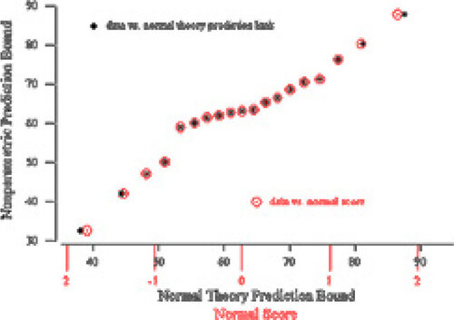
53 Comparing the two PIs leads to a natural question: When treating normally distributed data, how do these two prediction procedures compare? Given normal residual structure, the normal theory PI is preferred over the nonparametric PI (Hahn and Meeker 1991, pp. 75-76). However, Patel (1989, p. 2401) points out that there is little available information on this issue. Comparing the two methods (perhaps via simulation) seems a fruitful area of investigation for students in, say, mathematical statistics courses. Indeed, even the question “How should they be compared?” is worth taking up with an audience predisposed towards theory.

6. Summary

54 Prediction intervals are a success in my classroom. Students like this relatively concrete application; working with PIs builds confidence and provides learners with a measure of insight into a number of statistical procedures. With a PI, the data are used to make a formal inference in a way that is non-trivial (yet often computationally simple), is directly referenced by graphically displayed data, and makes use of fundamental statistical techniques. Finally, PIs form somewhat of a rallying point for my instruction. I find myself constantly referring to them in order to illustrate a variety of issues. Try teaching prediction intervals!

Appendix A:

Burn Times of Matches

The activity referred to in Section 3.1 requires of students a little time (say two minutes each), and of the instructor an extremely small investment in supplies. I use Ohio Blue Tip Kitchen Matches. The matches are notched about 5 mm from the bottom. Using either pliers or a vice, grip the match at the notch (assuring uniformity in the way the matches are positioned), orienting the match upright. A lighter ignites the match— ignition is marked by a very distinctive sound that triggers the start of a stopwatch. When the flame dies—again quite identifiable and accompanied by a distinctive wisp of smoke—the watch is stopped and the elapsed time recorded.

I prefer to have all students perform this experiment in the same conditions. My office is equipped with a makeshift vice, lighter, stopwatch, and a box of matches. Students stop by, I supply a few directions, a match is selected and set upright in the vice, I apply the lighter to the match head, and, upon ignition, the student begins timing. When the flame dies (the current low/high records are about 15/90 seconds), the watch is stopped, and the student records the burn time of the match to the nearest 0.01 second (overkill, but it prevents ties).

While the particular collection of 19 observations given in Table 1 show little evidence of nonnormality (see Figure 5), the larger collection I have accumulated markedly departs from normality in the form of substantial left skew.

Appendix B:

Minitab Macros

B.1 Prediction Intervals

The macro described below obtains two-sided PIs for univariate data in Minitab column C. I assume the macro is saved in the file p=redict.mac. Invoke it with

MTB > %predict C P

where P% is the confidence level. Six PIs are reported:

1.	A conservative exact two-sided nonparametric PI, at the smallest attainable level no less than P%.
2.	A liberal exact two-sided nonparametric PI, at the largest attainable level no greater than P%.
3.	An exact PI at level between those of the conservative and liberal PIs, formed with the lower endpoint of the conservative PI and upper endpoint of the liberal PI. This interval is two-sided but unbalanced by one position.
4.	An exact PI at level between those of the conservative and liberal PIs, formed with the lower endpoint of the liberal PI and upper endpoint of the conservative PI. This interval is two-sided but unbalanced by one position.
5.	An (approximate) P% two-sided PI, obtained by linear interpolation of the bounds given by the PIs of 1 and 2 above.
6.	The P% normal theory two-sided PI.

If an exact, balanced, two-sided nonparametric PI is attainable at the given level, it alone is produced in lieu of 1 through 5.

B.2 Percentiles

A second macro obtains a Pth percentile for univariate data in Minitab column C. I assume the macro is saved in the file p=ctile.mac. Invoke it with

MTB > %pctile C P

The definition of Section 3.2 is used to obtain the two nearest exact percentiles, as well as a linearly interpolated value for the Pth percentile. If the percentile is exactly attainable, it alone is produced. The macro is easily adapted to obtain one-sided prediction intervals.

Appendix C:

Textbook Coverage of Prediction

The textbooks I examined while preparing this article try very hard to get prediction right. My argument is rarely with what they do say, instead it is with how they say it and what they fail to mention. Often, considering a clientele of undergraduates with little statistical experience, the prose is quite difficult. A brief report of my observations follows.

The one-sample normal theory PI is formulated in Scheaffer and McClave (1990, p. 291), Devore (1995, p. 296), and Vining (1998, p. 176), using the right-most expression of (8). These texts, as well as Vardeman (1994) (discussed below), are calculus-based texts that target engineers.

Extensive coverage of prediction intervals, as well as tolerance intervals, is found in Vardeman (1994). The nonparametric PI of Section 3.1 is covered on pages 344-347. Treatment is confined to the minimum and maximum as bounds. This is reasonable when data are collected on a system operating in control; the extremes form natural control limits, and determining the confidence level achieved when using these limits is then important. The text also treats normal theory PIs for a number of models. While (6) is not implemented throughout, it does appear on page 553, in a discussion of how to construct a PI from software regression results. The text includes a wealth of PI exercises.

The expression for standard error of prediction given by (6) appears in Dielman (1991, p. 109)—not an introductory text.

Either (5), or something very similar, is found almost without exception in introductory statistics texts written with a broad, nonmathematically-oriented audience in mind. To list but a few: McClave et al. (1997, p. 511), Triola (1997, p. 513), Blaisdell (1998, p. 664), and Weiss (1999, p. 905); also—in an optional section on regression computations— Graybill et al. (1998, p. 267) and Moore and McCabe (1999, p. 690). All of these cited texts—and many others—limit the treatment of prediction to linear regression.

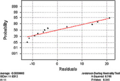
I found one example of inappropriate statistical practice. An example in Weiss (1999, pp. 872-908) regresses the price of the Orion model of automobile on age. A normal probability plot of the residuals is shown in Figure 6; this plot is duplicated on page 881 of the text. The normal theory PI (5) is used to predict the price of a three- year-old Orion. The discussion that accompanies the probability plot concludes “There are no obvious violations of the assumptions for regression inferences” (p. 881). I disagree: there is evidence that the residual structure is nonnormal. I am not at all convinced that regression inferences are appropriate—particularly predictive inferences. (It is questionable whether mean inference—using the usual methods—ought to be undertaken here. Certainly the nominal procedural levels must be taken with a grain of salt.)

Figure 6. Normal Probability Plot of Residuals. Price of the Orion model automobile is regressed on age; a normal probability plot of the residuals is displayed.

Textbooks take pains to distinguish the prediction interval from the confidence interval. The following is exemplary, and would work to even greater effect had (6) appeared in the accompanying section on regression calculations.

…the standard error…used in the prediction interval includes both the variability due to the fact that the least-squares line is not exactly equal to the true regression line and the variability of the future response variable…around the subpopulation mean. (Moore and McCabe 1999, p. 676)

Isn’t this exactly what (6) states?

Graybilletal.(1998) omit the traditional PI formula from the text proper, including it only in an appendix. This text’s notation distinguishes between the prediction function, denoted Y(x), and the mean function ${\mu }_y(x)$. It is assumed that students will use statistical software to do the computations.

Triola (1997, pp. 513 and 517) produces the standard error of prediction in the text proper, relegating the standard error of an estimated mean to an exercise.

Explaining the traditional formula (5) results in some interesting reading, particularly when it is contrasted with the corresponding formula (9) for the standard error of an estimated mean.

Notice that the only difference in the formulas is the inclusion of a 1 under the radical in the error bound for the prediction interval. (Blaisdell 1998, p. 664)

True enough. Yet the number 1 is hardly important—it is the application of 1 to the residual standard deviation that matters. Here’s a very similar statement.

Note that the only difference between the recipes for these two standard errors is the extra 1 under the square root sign in the standard error for prediction. This standard error is larger due to the additional variation of individual responses about the mean response. (Moore and McCabe 1999, p. 690)

The formula for standard error of prediction is then produced, with a reference directing the reader to the following note: “This quantity is the estimated standard deviation of $\widehat{y}-y$, not the estimated standard deviation of $\widehat{y}$ alone” (Moore and McCabe 1999, p. 709). While this does address the quantity ($\widehat{y}-y$) a statistician would work with in deriving the PI, I suspect it in no way guides the intended reader.

The following strikes me as quite difficult reading.

The error in estimating the mean value of y, E(y), for a given value of x, say x_p, is the distance between the least square line and the true line of means, $E\left(y\right)={\beta }_0+{\beta }_{1}x$. This error, $\left[\widehat{y}-E\left(y\right)\right]$, is shown in [a figure not reproduced here]. In contrast, the error $$\left(y_p-\widehat{y}\right)$$ in predicting some future value of y is the sum of two errors—the error of estimating the mean of y, E(y) … plus the random error that is a component of the value of y to be predicted… (McClave et al., 1997, pp. 513-514)

Finally, one incorrect statement.

If you examine the formula for the prediction interval, you will see that the interval can get no smaller than $\widehat{y}\pm z_{\alpha /2}\sigma$. (McClave et al. 1997, p. 516)

While the PI converges in probability to the specified interval, the observed PI margin of error, $t_{\alpha /2}s.e.p.(Y)$, can be less than the population margin of error, $z_{\alpha /2}\sigma$, due to sampling variability.

References

- Blaisdell, E. A. (1998), Statistics in Practice (2nd ed.), Fort Worth, TX: Saunders.
- Devore, J. L. (1995),Probability and Statistics for Engineering and the Sciences (4th ed.), Belmont, MA: Duxbury Press.
- Dielman, T. (1991), Applied Regression Analysis for Business and Economics, Boston: Duxbury.
- Graybill, F. A., Iyer, H. K., and Burdick, R. K. (1998), Applied Statistics: AFirst Course In Inference, Upper Saddle River, NJ: Prentice Hall.
- Gumbel, E. J. (1939), “La Probabilité des Hypothèses,” Compes Rendus de l’ Académie des Sciences (Paris),209,645–647.
- Hahn, G. J. (1970), “Statistical Intervals for a Normal Population,” Journal of Quality Technology, 2, 115-125, 195–206.
- Hahn, G. J., and Meeker, W. Q.(1991), Statistical Intervals: A Guide forPractitioners, New York, NY: Wiley.
- Hyndman, R. J., and Fan, Y. (1996), “Sample Quantiles in Statistical Packages,” The American Statistician, 50, 361–364.
- Mc Clave, J. T., Dietrich, F. H., and Sincich, T. (1997), Statistics (7th ed.), Upper Saddle River, NJ: Prentice Hall.
- Moore, D. S., and McCabe, G. P. (1999), Introduction to the Practice of Statistics (3rd ed.), New York, NY: Freeman.
- Neter, J., Kutner, M. H., Nachtsheim, C.J., and Wasserman, W. (1996), Applied Linear Statistical Models (4thed.), Chicago, IL: Irwin.
- Patel, J. K. (1989), “Prediction Intervals—A Review,” Communications in Statistics—Theory and Methods, 18, 2393–2465.
- Scheaffer, R. L., and Mc Clave, J. T. (1990), Probability and Statistics for Engineers (3rd ed.), Boston, MA:PWS-Kent.
- Scheuer, E. M. (1990), “Let’s Teach More About Prediction,” in Proceedings of the Statistical Education Section, American Statistical Association, pp. 133–137.
- Triola, M. F. (1997), Elementary Statistics (7th ed.), Reading, MA: Addison Wesley.
- Vardeman, S. B. (1992), “What About the Other Intervals?,” The American Statistician, 46, 193–197.
- Vardeman, S. B.– (1994), Statistics for Engineering Problem Solving, Boston, MA: PWS.
- Vining, G. G. (1998), Statistical Methods for Engineers, Pacific Grove, CA: Duxbury.
- Weibull, W. (1939), “The Phenomena of Rupture in Solids,” Ingeniors Vetenskaps Akademien Handlinger, 153, 17.
- Weiss, N. A. (1999), Introductory Statistics (5th ed.), Reading, MA: Addison Wesley Longman.
- Whitmore, G. A. (1986),”Prediction Limits for a Univariate Normal Observation,” The American Statistician, 40, 141–143.
- Wilks, S. S. (1941), “Determinationof Sample Sizes for Setting Tolerance Limits,” Annalsof MathematicalStatistics, 12, 91–96.