A Simplified Introduction to Correlation and Regression

Abstract

The simplest forms of regression and correlation involve formulas that are incomprehensible to many beginning students. The application of these techniques is also often misunderstood. The simplest and most useful description of the techniques involves the use of standardized variables, the root mean square operation, and certain distance measures between points and lines. On the standardized scale, the simple linear regression coefficient equals the correlation coefficient, and the distinction between fitting a line to points and choosing a line for prediction is made transparent. The typical size of prediction errors is estimated in a natural way by summarizing the actual prediction errors incurred in the dataset by use of the regression line for prediction. The connection between correlation and distance is simplified. Despite their intuitive appeal, few textbooks make use of these simplifications in introducing correlation and regression.

Keywords:

• Distance
• Prediction error
• Root mean square
• Standard deviation
• Standardized variables

1. Introduction

1 The introduction to association between two quantitative variables usually involves a discussion of correlation and regression. Some of the complexity of the usual formulas disappears when these techniques are described in terms of standardized versions of the variables. This simplified approach also leads to a more intuitive understanding of correlation and regression. More specifically, the following facts about correlation and regression can be simply expressed.

2 The correlation r can be defined simply in terms of standardized variables zx and zy as $r={\displaystyle \sum z_x{z}_y/n}$. This definition has the advantage of being described in words as the average product of the standardized variables. No mention of variance or covariance is necessary for this. The regression line zy = r zx is simple to understand. Moreover, the tendency of regression toward the mean is seen to depend directly on r. The appearance of a scatterplot of standardized variables depends only on r. The illusion of higher correlation for unequal standard deviations is avoided. The prediction error of a regression line is the distance of the data points from the regression line. These errors may be summarized by the root mean square of the vertical distances: for standardized variables this is $\sqrt{1-r^{{}^2}}$. Correlation is related to the perpendicular distances from the standardized points to the line of slope 1 or -1, depending on the sign of the correlation. In fact, the root mean square of these perpendicular distances is $\sqrt{1-|r|}$.

3 The key to these simplifications and interpretations is an understanding of the standardization process. For this it is necessary for students to understand that a standard deviation really does measure typical deviations. This is aided by the use of the “n” definition of the standard deviation: $$s=\sqrt{\frac{1}{n}{\displaystyle \sum _{i=1}^n{\left(x_i-\overline{x}\right)}^2}}$$

It is apparent that this is the average squared deviation, and taking the square root of this is a natural step to recover the original units. So a standardized observation $\frac{\left(x_i-\overline{x}\right)}{s}$ is the number of these “typical” deviations that an observation is from the mean. This describes the measurement relative to the (sample) distribution from which it comes.

4 For students who must deal with traditional courses and textbooks using a strictly formula-based approach, it may be necessary to use the suggestions here in a first introduction. Once this simple introduction is accomplished, the more traditional approach could still be used, and shown to yield essentially the same results. The simplified introduction gives an easy-to-absorb sense of the strategy, and statistical software can take care of the slightly different arithmetic that working with standardized variables entails. The simplified approach suggested here has been used in many semesters of an introductory course based on the text by Weldon (1986), and no n vs. n - 1 confusion has been noted by the students or by instructors of subsequent statistics courses.

2. Details

5 The definition $$r={\displaystyle \sum z_x{z}_y/n}$$ assumes that the “n” definition of the standard deviation is used. A similar definition using the “n - 1” definition of the standard deviation would require the n in the denominator to be replaced by n - 1. To be able to describe the correlation as the average product of the z’s not only simplifies the formula, but allows the student to think of the scatterplot quadrants as determining the correlation. The effect of outliers can be gauged more simply than with the original units formula.

6 It is important for students to realize that the regression line is not a simple curve fit to the points, but rather a line designed for prediction. The formula $$z_y=rzx$$ makes this quite clear since the “point-fit” line $z_y=z_x$, which minimizes the sum of squares of the perpendicular distances, is usually a line of greater slope than the regression line. (Freedman, Pisani, and Purves 1998 call zy = zx the SD line.) Moreover, the prediction lines $$z_y=r{z}_x$$ and $$z_x=r{z}_y$$ (or zy = (1/r) zx) are clearly not the same line. Another effect simplified by this approach is that of regression toward the mean, with the predicted zy less extreme than zx.

7 Regression predictions can be made with the regression equation expressed in original units, but the direct use of zy = r zx seems a viable alternative. The given value of X is easily converted into a zx value, the prediction zy can be simply obtained, and then zy can be converted back into original units. While this involves a bit more arithmetic, the conceptual simplicity involving only the standardization idea and the r multiplier make this approach preferable for the novice. Note also that the error of prediction can be found on the z scale using $\sqrt{1-r^2}$, and can then be transformed back to original units.

8 It is well known that stretching one scale of a scatterplot can increase the apparent correlation (even though the correlation is actually unchanged). Portraying data in their standardized scale removes this illusion. It also makes the point that the correlation does not depend on the scales of the variables. Moreover, “banking to 45o” (that is, choosing an aspect ratio for the plot that portrays trends as close to ± 45o as possible) is recommended for graphical assessment (Cleveland 1993).

9 The distance of a point (x0, y0) to a line y = r x in the direction of the y axis is | y0 - r x0 |. Thus for standardized variables, the root mean squared distance is $\sqrt{\frac{1}{n}{\displaystyle \sum {\left(z_y-r{z}_x\right)}^2}.}$. Expanding and using $\frac{1}{n}{\displaystyle \sum z^2=1}$ produces the well-known result that the root mean square distance of the data from the regression line is $\sqrt{1-r^2}$ times the standard deviation, which in this case is 1. The condition $\frac{1}{n}{\displaystyle \sum z^2=1}$ only depends on the use of the “n” definition for the standard deviation—with the “n - 1” definition of r and the standard deviation, the same result is true.

10 The minimum (i.e., orthogonal) distance of a point (x0, y0) to a line ax + by + c = 0 is | ax0 + by0 + c |/(a2 + b2)1/2. The line of slope “sign of r” = sgn(r) in standard units is zx - (sgn(r)) zy = 0, and the distance of a point (zx, zy) to this line is therefore $$\frac{\left|z_x-\left(\mathrm{sgn}(r)\right)z_y\right|}{\sqrt{2}}.$$

The root mean square of these distances is $$\frac{1}{\sqrt{2}}{\left(\frac{\left({\displaystyle \sum z_x^2+{\displaystyle \sum z_y^2-2\mathrm{sgn}(r){\displaystyle \sum z_x{z}_y}}}\right)}{n}\right)}^{1/2}=\sqrt{1-\left|r\right|}.$$(1)

This result appeared in Weldon (1986).

3. “n” Definition of Sample Standard Deviation

11 This “n” definition simplifies many things in teaching statistics. The justification for the more common “n - 1” definition is based on the unbiasedness of s2 for estimating ${\sigma }^2$, which is not really relevant for estimation of $\sigma$. One could even question the need for unbiasedness when it costs us in terms of mean squared error. The “n” definition is easier to explain and has smaller mean squared error.

12 Some instructors are reluctant to use the “n” definition of the sample standard deviation because it complicates the discussion of the t-statistic. But actually, if the t-statistic is defined in terms of the “n” definition of the sample standard deviation, the divisor “n - 1” appears in its proper place as a degrees-of-freedom factor, preparing the student in a natural way for the chi-square and F-statistics: $$t=\frac{\left(\overline{x}-\mu \right)}{s/\sqrt{n-1}}$$

. The s in this formula is $$s=\sqrt{\frac{1}{n}{\displaystyle \sum _{i=1}^n{\left(x_i-\overline{x}\right)}^2}}$$

as before. Nevertheless, for instructors who wish to stick with the “n - 1” definition, the approach to correlation and regression given in the rest of this paper will still hold together.

13 Another reason for avoiding the n definition is the confusion that might be caused by the majority preference for the n - 1 definition in other textbooks. However, once the idea of standard deviation is understood through the simplest approach, the existence of variations may not be so disturbing. The n - 1 definition can be viewed in regression contexts as an “improvement” on the n definition, and its extensions to the multi-parameter case will likely be accepted without too much consternation.

4. An Example

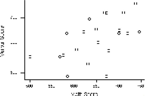
14 To illustrate the above formulas, consider the following dataset relating performance on a mathematics test with performance on a verbal test. The data were sampled from a larger dataset in Minitab (1994). The first step for the student is to plot the data. Using the default scaling, Minitab produces the plot in Figure 1.

Figure 1. Scatterplot of “Grades” Data from Minitab. The scaling is the default scaling used by Minitab.

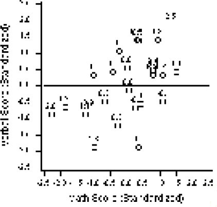
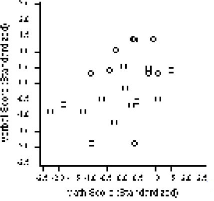
15 If the variables are centered, and the scales equalized, we obtain the plot in Figure 2. On this scale, it can be seen that the perpendicular distances of the points from the line of slope one (which may be called the point-fit line or the SD line) are usually less than one but greater than 0.5. Equation (1)$$\frac{1}{\sqrt{2}}{\left(\frac{\left({\displaystyle \sum z_x^2+{\displaystyle \sum z_y^2-2\mathrm{sgn}(r){\displaystyle \sum z_x{z}_y}}}\right)}{n}\right)}^{1/2}=\sqrt{1-\left|r\right|}.$$(1) says that the root mean square of these distances is equal to $\sqrt{1-\left|r\right|}$. In this case, the sample correlation r is approximately 0.5, so the root mean square distance is 0.7, which is about what we expect from visualizing the graph.

Figure 2. Equal-Scales Scatterplot of “Grades” Data. Both scales are in standardized units.

16 Another observation that can be made from the graph concerns the average product. The average product is the correlation, and the idea of this can be gleaned from a graph like Figure 3, in which the points are annotated with the product of the standard scores. The fact that the average product is 0.5 is not obvious, but one can at least see which quadrants must have the largest contributions to the average in order that the correlation be positive.

Figure 3. Pointwise Contributions to the Correlation Coefficient. The average of these zxzy contributions is the correlation coefficient.

17 Another feature of the “average product” definition of the correlation is the ability to detect outliers. From the graph it can be observed that a point at (-1.5, 1.5) would seem not to belong to the oval shaped scatter, even though the individual values of -1.5 and 1.5 on either variable are not unusual. Such a point would be in the extreme lower tail of a dotplot of the products of the standardized variables, confirming from this definition of correlation that the point is unusual. Note that the addition of this one point would reduce the sample correlation from .50 to .38.

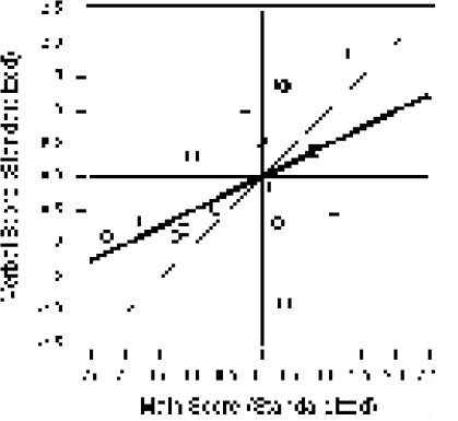
18 The regression line for predicting the verbal score from the math score is, in the standardized scale, zV = r zM; it is shown graphically in Figure 4. This graph shows clearly the difference between the “point-fit” line and the regression line for predicting V from M. Moreover, the line for predicting M from V is clearly a different line.

Figure 4. Regression Line and Point-Fit Line. The point-fit line is “closest” to the data points.

19 As a final step in using the zV = r zM regression equation, it is necessary to convert the regression line back to the original units. First we need to record the mean and standard deviation (SD) of each variable: mean(V) = 619, SD(V) = 71; mean(M) = 649, SD(M) = 65. Then, substituting directly into zV = r zM, one gets (V - 619)/71 = 0.5(M - 649)/65. For example, if M = 700, the right side is 0.5(51)/65 = .39, so that the predicted V is 619 + .39(71) = 647. For many predictions, one may need the explicit equation V = 619 + 71(0.5)(M - 649)/65, which simplifies to V = 265 + .54M. Compared to the arithmetic of formulas for the intercept and slope, which tend to obscure the operation, this is relatively straightforward.

5. Related Work

20 Most textbooks introduce correlation and regression via formulas. For example, Moore and McCabe (1993, p. 164) and Wild and Seber (2000, p. 540) use the n - 1 definition of the correlation and define the regression slope in terms of the unstandardized variables (Moore and McCabe 1993, p. 123; Wild and Seber 2000, p. 518).

21 The explicit interpretation of correlation in terms of distance does not appear in the “Thirteen Ways” summary article by Rodgers and Nicewander (1988), nor in the follow-up papers by Rovine and von Eye (1997) and Nelsen (1998), even though this interpretation appears to be one of the most intuitive.

6. Summary

22 When data are expressed in standardized form, correlation and regression methods can be described very simply. The difference between fitting a line to points and regression is clarified by this simpler presentation. The use of n - 1 in formulas for the standard deviation and the correlation coefficient is an unnecessary complication.

Acknowledgments

The author would like to thank the referees, the editor, and an associate editor for helpful comments on the first draft.

References

- Cleveland, W. S. (1993),Visualizing Data, Summit, NJ: Hobart Press, p. 89.
- Freedman, D., Pisani, R., and Purves, R. (1998), Statistics (3rd ed.), New York: Norton.
- Minitab Inc. (1994), MINITAB Reference Manual, Release 10Xtra, State College, PA: Author.
- Moore, D. S., and McCabe, G. P. (1993), Introduction to the Practice of Statistics (2nd ed.), New York: Freeman.
- Nelsen, R. B. (1998), “Correlation, Regression Lines, and Moments of Inertia,” The American Statistician, 52, 343–345.
- Rodgers, J. L., and Nicewander, W. A. (1988), “Thirteen Ways to Look at the Correlation Coefficient,” The American Statistician, 42, 59–66.
- Rovine, M. J., and von Eye, A. (1997), “A 14th Way to Look at a Correlation Coefficient: Correlation as the Proportion of Matches,” The American Statistician, 51, 42–46.
- Weldon, K. L. (1986), Statistics: A Conceptual Approach, Englewood Cliffs, NJ: Prentice-Hall, p. 144.
- Wild, C. J., and Seber, G. A. F.(2000), Chance Encounters: A First Course in Data Analysis and Inference, NewYork: Wiley.