 ?Mathematical formulae have been encoded as MathML and are displayed in this HTML version using MathJax in order to improve their display. Uncheck the box to turn MathJax off. This feature requires Javascript. Click on a formula to zoom.
Abstract
Sampling distributions are central to understanding statistical inference, yet they are one of the most difficult concepts for introductory statistics students. Although hands-on teaching methods are preferred, finding the right balance between theory and practical experience has not been easy. Simulation activities have not always captured the research situations that statisticians work with. This paper describes a method developed by the author to teach sampling distributions using a collaborative learning simulation based on political polling. Anecdotally, students found the polling scenario easy to understand, interesting, and enjoyable, and they were able to explain the meaning of sample results and inferences about the population. Sample examination questions are included, with examples of students' responses that suggest that the method helped them to understand sampling error and its role in statistical inference.
1. Introduction
1 Sampling distributions are central to statistics because they underlie statistical inference. Yet sampling distributions, because of their theoretical nature, are one of the most difficult concepts for beginning students to grasp (CitationZerbolio 1989). Even when students are able to solve conventional textbook problems, they may not understand the underlying concepts; in fact, knowing a procedure alone may discourage the search for more relational understanding (CitationPollatsek, Lima, and Well 1981). Therefore, it is essential that students be introduced to important statistical concepts in a form that is intuitively meaningful to them.
2 Many methods have been proposed for teaching statistical concepts. The consensus is that it is better to introduce topics through hands-on activities and simulations rather than through theoretical descriptions (CitationDyck and Gee 1998, CitationGarfield and Ahlgren 1988, CitationRossman and Chance 1999). But for sampling distributions – one of the most theoretical concepts in introductory statistics – finding the right balance between theory and concrete experience has been more difficult than one might expect. One approach has been to have students “imagine” concrete objects such as marbles or chips from which samples are drawn (CitationZerbolio 1989). That is, students imagine the population as a big bag of marbles, each with an IQ score printed on it. Samples of marbles are randomly drawn from the bag and placed in a glass; the mean of all the IQ’s in the glass is written on a chip that represents that glass. Chips representing many glasses are then gathered together in a new bag to represent the sampling distribution. CitationZerbolio (1989) stated his preference for imagination rather than physical experience with manipulating objects because, in his view, a hands-on simulation implies finite limits to infinite populations and the infinite number of samples that may be drawn from them.
3 A popular, more hands-on approach has been to have students draw samples from a large bag of candies such as M&M;’s or Reese’s Pieces to estimate the proportion of candies of a particular color and to study sampling variability (CitationDyck and Gee 1998, CitationRossman and Chance 1999). In an experimental study comparing the candy method to the imagination method, students taught by the candy method performed better on a quiz and also rated their enjoyment of the course higher than students taught by the imagination method (CitationDyck and Gee 1998).
4 More recent methods for teaching sampling distributions have involved computer simulation software (CitationdelMas, Garfield, and Chance 1999). In one study, prior to using the software program, students did a hands-on simulation in which they drew samples from a population to estimate first-term grade-point averages or the dates of pennies. After this, students used a specially developed software package in which they drew repeated random samples from a population to explore the resulting sampling distributions when population characteristics and sample sizes varied. The authors discovered that the computer simulation itself did not guarantee that students developed the correct conceptual understanding of sampling distributions (as measured by a pre- and posttest). However, they also discovered that students learned more from using the software simulation if they formed and tested predictions and were confronted by evidence that contradicted their misconceptions. Future research will include investigation of whether hands-on experiences prior to using the simulation software can facilitate learning from the simulations. These findings demonstrate the value of making activities concrete, and are also consistent with the recommendation by CitationRossman and Chance (1999) that a physical, hands-on simulation precede activities with computer simulations to help students connect the ideas with the technology, which may not automatically occur with technology alone.
5 Although these approaches have successfully used physical and computer-generated simulations to teach sampling distributions, there is still work to be done designing meaningful simulation activities that relate more closely to the kinds of research situations that statisticians work with. In searching for a method to make sampling distributions concrete and accessible to beginning students, as well as related to real statistical research, I chose to create an activity related to political polling. Political polls are familiar and newsworthy, and there is always a fresh supply of current material on which to base lessons (see, for example, http://www.gallup.com and http://www.people-press.org, which are updated weekly). Polls provide topics for interesting discussions on population trends and how to measure them. In my experience, students relate to them easily and are interested and enthusiastic because they can analyze not only the simulation data but what the data say about the meaning of real polls on issues that interest them.
2. Instructional Activities
2.1 Students
6 The activity described here was first carried out in two sections of a required introductory statistics course for undergraduate business majors at a public four-year college in New York City during the Fall 1999 semester. Seventy students, all at the sophomore or junior level, participated. The course has a prerequisite of discrete math. The activity was repeated later that semester with 32 students in another section of the same course and with 26 students taking a required introductory statistics course at a public community college, where students have previously taken only elementary algebra, have difficulty relating to abstract mathematical concepts, and often suffer from math anxiety. The student-generated data from the simulation activity are reported for the initial group, which was the largest. The activity has since been repeated with other senior and community college classes in the spring and summer of 2000, with essentially the same outcomes.
2.2 Instructional Materials
7 Students were provided with text materials consisting of four lessons on several aspects of political polling: using a sample to represent a population; writing balanced poll questions; sampling variation and the margin of error; and exit polling practices. (A revised version of these materials may be viewed on http://www.pbs.org/democracy/buildyourowncampaign/lesson_plans.html, lessons 6, 7, 8, and 16.) Each lesson includes a link to a simple text explanation, examples drawn from actual polls, and activities for students. Most of the activities require students to discuss the concepts as they apply to a real or hypothetical polling scenario. For example, students may evaluate whether a proposed sampling procedure is representative, discuss why different versions of the same question used in actual polls elicited different responses, or draw conclusions from a published survey or exit poll. The activity for sampling distributions requires students to perform a simulation in which they draw repeated random samples from a box of tags representing a population of responses to a poll question, and then plot the results of their repeated samples and study the characteristics of the sampling distribution that was generated.
2.3 Procedure
8 Early in the semester, the class discussed sampling: why it is necessary, various sampling methods (simple random, systematic, stratified, and cluster) and their representativeness, and how sampling is used in polls and opinion surveys. Students also discussed issues in the wording of poll questions, evaluated the possible effects of different question wordings, and wrote questions that they would later use in their own data-collection projects. After covering probability and the normal distribution, we returned to sampling in the context of a real poll. I chose the United States Senate race in New York State, which was at the time between First Lady Hillary Rodham Clinton and New York City Mayor Rudolph Giuliani. The race was current, highly publicized, historically noteworthy (as the first time a First Lady has ever run for elective office), and of interest to students as residents of New York City with knowledge and strong feelings about both candidates.
9 We began our discussion of inference from samples with a few early polls showing a very close race. Some polls showed Clinton having a slight lead, others showed Giuliani leading, but all were too close to call. As students looked at the poll results, I posed questions: How can polls taken around the same time, all using random sampling, suggest different conclusions about who is leading? How accurate are sample results and what is the “margin of error”? How can we know when a front-runner can be projected as opposed to when a race is in a “dead heat”? In response to these questions, students generated the idea in discussion that sample results are only an approximation of true population preferences simply because when you poll a sample, you are not asking everybody in the population, and each sample is a different group of people. They inferred that the margin of error must be some kind of allowance for the fact that sample results are, at best, an imperfect measure.
10 The next phase was a hands-on, collaborative learning activity to demonstrate what happens when a pollster takes random samples to estimate a population preference. I had students divide into teams of four and told them that they were going to become pollsters for a day, to simulate an actual poll that stated that, nationwide, 48% of American voters favored having Hillary Rodham Clinton run for the United States Senate (CitationPew Research Center for the People and the Press 1999). If 48% of the population wanted her to run, how likely would it be that a pollster would find that exactly 48% of a sample would say they wanted her to run? If a sample found a percentage other than 48%, how far off would the sample be likely to be? To explore these questions, each team received a “mini-population” in the form of a box containing 100 tags, 48 of them marked “yes” and 52 of them marked “no.” Taking turns, each team member was to select repeated random samples of ten tags and record the proportion of yeses in each sample, replacing each sample before drawing a new one. The teams generated as many samples as they could in about twenty minutes, pooled the results for their group, and turned them in to be combined with those of the whole class. Each class of 35 students collectively generated approximately 110 samples.
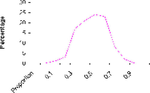
11 At the next session I distributed a frequency and percentage distribution combining the sample proportions collected by both classes so as to maximize the total number of samples, and we plotted a percentage polygon for the data (see and Figure 1). I introduced the formula for the standard deviation of the proportion, with a brief explanation of the standard deviation of binomially distributed data. (Our courses do not include the binomial distribution; if that is included, the derivation of the formula is clearer to students, but I have found that it is not essential to their understanding of the idea of sampling variation.) Then we observed the mean of the sampling distribution that we generated – it was almost exactly equal to the original population value we wished to estimate – and counted the percentages of our sample proportions that came within one and two standard deviations of the mean. These came out to 68% and 96%, respectively. This allowed us to discuss what happens when repeated samples are drawn from the same population: individual sample statistics do not always match the true population value, but vary and converge around it. Furthermore, after enough samples are accumulated, the distribution of sample proportions is approximately normal. Knowing this is extremely useful when one wishes to estimate the probability of obtaining a sample within a specified range of the population parameter, without having to take repeated samples every time.
Table 1. Random Samples of Size 10 Drawn from a Population of 100, 48% Yes
Figure 1. Sampling Distribution of Sample Proportion for Repeated Samples of Size 10.
12 This demonstration naturally led to a discussion of the margin of error as it is computed in political polls – as a give-or-take amount of variation that covers 95% of the sampling distribution in a particular situation – and to confidence intervals as an expression of the boundaries suggested by the margin of error (CitationBaumann and Danielson 1997). Examining the formula for the margin of error also led to a discussion of the effect of sample size (since pollsters obviously use samples larger than ten). We could see that the larger the samples taken, the smaller the sampling variation and the margin of error, and that the population size is not a factor in the margin of error. Once these ideas were clear, students could understand applications such as projecting winners in elections or comparing the responses of subgroups such as men and women: How much of a difference has to be observed in sample data in order to conclude with reasonable certainty that there is a difference in the population? What does the 95% refer to? What is the chance of ending up with sample data that lead to the wrong conclusion, and what could pollsters do to make this outcome less likely? To illustrate this latter point, we moved on to the lesson on exit polling practices and discussed how care is taken to minimize the risk of an erroneous projection by choosing a larger sample (stratified by voting precincts around the state or the country) and using a larger confidence coefficient (99.5%).
13 When students were clear on the meaning of sampling distributions and the margin of error in polls, they were ready to consider the sampling distribution of the mean and the Central Limit Theorem. I proposed that we could demonstrate the same principles of sampling variation by collecting each student’s height in inches on a card, putting all the cards in a bowl, and repeatedly selecting random samples of cards. Then we could compute the mean height for each sample and plot the sample means to see how they distribute around the mean for the entire class. While this can be done as an additional classroom exercise, I have found that when I relate it back to the polling exercise, students resonate and do not need to have it demonstrated again. This led directly to our remaining topics: confidence intervals for the mean, statistical process control (which involves repeated sampling to estimate a population mean or proportion), hypothesis testing, and Type I and Type II errors.
3. Outcomes
14 A quantitative comparison of students’ performance before and after I adopted this method is difficult because, as noted previously, students can often answer traditional textbook problems without necessarily having a deep understanding of the underlying concepts. That has certainly been the case with many of our students. Before adopting this method I tested students in the traditional manner (presenting problems to be worked out mathematically with little explanation required); I now find these tests inadequate. Anecdotally, I have found that since I adopted the new method, classroom climate has greatly improved and students have satisfactorily answered examination questions that require them to explain their reasoning more fully than they did when taught by the old method. Previously, they often had difficulty just stating a conclusion about whether to reject a null hypothesis. To provide some insight into the improvements I have observed in students’ reasoning, in the next sections I describe their reactions to the new method and present some exam questions that they are now able to answer successfully, along with some of their responses.
3.1 Students’ Reactions
15 First, students show much greater interest in the class discussion when I introduce polls. They participate more actively and comment on their intuitive reactions to the poll results, which helps them relate more easily to the underlying mathematical and statistical concepts. This is especially valuable in the community college statistics class, where students routinely have a high degree of mathematics and statistics anxiety and are reluctant to trust their own intuitions, even when they are correct (CitationGourgey 1992). There is no longer the heavy silence that is so often present when students feel passive, lost, or afraid to say something that may sound stupid, nor are there as many anxious requests to have concepts repeated several times because they were unable to follow them. At the end of the semester, they consistently rate the “real-life examples” as one of the most interesting parts of the course.
16 Moreover, students show a high degree of enthusiasm with the collaborative learning exercise. They seem to enjoy actually doing something to see what happens rather than just having to take the laws of statistics on faith. When we put the class-wide data together and saw the shape of the distribution, the normal curve was no longer just a theory, and sampling variation became something that statisticians have to wrestle with when they try to draw accurate conclusions. Statistics is by nature an experimental discipline, and it should be taught that way as much as possible.
17 Even with this exercise, the sampling distribution remains a difficult concept for students to understand. I found I had to keep reiterating, as we moved to subsequent topics, the difference between the population distribution and the sampling distribution, and which one we were working with at any given moment. However, any time I sensed students’ confusion, I was able to remind them of our sampling activity and what we demonstrated, and that cleared up the confusion quickly as students expressed recognition and relief – two reactions that I rarely saw when I used only a theoretical presentation.
3.2 Assessment
18 On examinations, I now include questions asking students to explain the results of a poll, whether an observed difference in a sample signifies a true difference in the population, and what the standard error and the margin of error represent. They must explain these concepts in their own words, as well as demonstrate them with statistical evidence. Some sample questions are presented in Table 2. Most of my students, including the community college students, were able to do this well. Much less frequently than before did I see students who were able to compute a statistical formula, but unable to draw a conclusion from their results. The responses presented below were collected from a community college class of 24 students in Spring 2000; their responses were comparable to those of the senior college students, and are particularly noteworthy because community college students are the ones who have the most difficulty understanding statistical concepts and the poorest grades in statistics.
Table 2. Sample Examination Questions on Polling
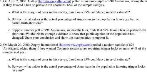
19 Students were taught the formula for the margin of error of a proportion based on the 95% confidence interval for one sample, because that is the form most frequently reported in pre-election polls in order to make interpretation simpler for the public (CitationBaumann and Danielson 1997). A more precise analysis would construct a confidence interval for the difference in proportions, but checking for overlap of the individual confidence intervals is simpler for students to understand and constitutes a reasonable and conservative alternative. The assessment goal was to determine whether students understood the idea of sampling error and its use in drawing an inference about a population from a sample. To get full credit, students had to show their mathematical work and explain their conclusions in complete sentences. There were two alternate forms of the exam, each containing one of the questions in Table 2, so half the class responded to each question.
20 Eighteen out of 24, or 75%, of the community college students received full credit for their responses. All showed the confidence intervals they constructed, and many also graphed the two intervals to show whether the intervals overlapped, as had been demonstrated in class. Typical explanations for the partial-birth abortion polls, for which the difference was significant, were as follows:
This should be enough evidence that the public opinion has changed, because the percentages don’t overlap. There is a separation, as you can see (between the intervals in the graph, shown).
It is not overlapping because there is a gap (between the intervals in the graph, shown). People’s opinion did change. Less people are in favor of a partial-birth abortion ban afterward.
The evidence would show that public opinion has changed because there is no overlap, therefore there is a clear difference.
21 Typical explanations for the trigger lock polls, for which the difference was not significant, were the following. The last response is unusually articulate and shows how the student has been able to draw all the concepts together.
No, this would not be enough evidence to show a change. There is not a clear answer here because the poll numbers overlap. There is no difference.
No, it would not be enough to show a change because it would be overlapping so you wouldn’t be able to say whether or not a change took place or that it was a sampling error.
There is not enough evidence to show that public opinion has changed. Due to the 3% margin of error there are overlapping positive responses and we cannot conclude that the opinion has changed.
Since the values overlap, there isn’t enough evidence to indicate any change at all. The results are “too close to call.” If the sample size for both surveys was larger, the margin of error would drop and perhaps then the results would show a meaningful difference.
22 These responses indicate that most of the students have correctly grasped that it is necessary to take sampling error into account when evaluating sample data. The students who got these questions wrong made the error of comparing the sample percentages as if they could be taken literally without allowing for sampling error, saying there has been a change in opinions simply because the percentage fell from the first survey to the second. These responses are certainly more satisfactory than those I used to observe when teaching sampling distributions theoretically, when students simply constructed a confidence interval, or computed a hypothesis test and then had difficulty explaining whether to reject the null hypothesis. I am continuing to work on developing test questions that tap more deeply into students’ understanding of the sampling distribution itself, to be certain that they grasp what it is and how it is related to – but different from – a population distribution.
4. Conclusions
23 Teaching sampling distributions using the polling simulation, in the context of actual statistical research, has not only worked well for my students, but has made teaching more satisfying for me as well. Statistical inference has been much easier to teach after using this exercise. I see fewer confused looks, class discussions are livelier and go more smoothly, and there are fewer expressions of frustration and requests that I repeat explanations. Students have told me afterward that they really enjoyed the class; particularly at the community college, students said that the class had calmed their fears that statistics would be too hard for them. Hands-on exercises based on current statistical practice show great promise, especially for students who have limited mathematical skills and a high degree of anxiety about the subject. Now that preliminary classroom trials using this method have elicited positive student responses both in class and on exams, formal evaluation comparing different instructional methods, with additional question types, would provide objective data to support the method’s benefits over traditional instruction that focuses primarily on theory.
Acknowledgments
I would like to thank the staff of the Pew Research Center for the People and the Press, Washington, DC, and of the Voter News Service, New York, NY, for their willingness to be interviewed about the methods they use to conduct political and exit polls. This information served as the knowledge base for constructing the polling lessons used in my courses. I would also like to thank the reviewers and associate editor for their comments, which improved the readability and content of the paper.
References
- Baumann, P. R., and Danielson, J. L.(1997), “Statistics in Political Polling,” Stats: The Magazine for Students of Statistics, No. 20,Fall, 8–12.
- delMas, R. C., Garfield, J., and Chance, B. L. (1999), “A Model of Classroom Research in Action: Developing Simulation Activities to Improve Students’ Statistical Reasoning,” Journal of Statistics Education [ Online], 7(3). (http://www.amstat.org/publications/jse/v7n3/delmas.cfm)
- Dyck, J. L., and Gee, N. A. (1998), “A Sweet Way to Teach Students About the Sampling Distribution of the Mean,” Teaching of Psychology, 25(3), 192–195.
- Garfield, J., and Ahlgren, A.(1988), “Difficulties in Learning Basic Concepts in Probability and Statistics: Implications for Research,” Journal for Research in Mathematics Education,19(1), 44–63.
- Gourgey, A. F. (1992), “Tutoring Developmental Mathematics: Overcoming Anxiety and Fostering Independent Learning,” Journal of Developmental Education, 15(3), 10–14.
- Pew Research Center for the People and the Press (1999), “Front Loading and Frontrunners Notwithstanding: It’s Still too Early for the Voters” [ Online], June 16. (http://www.people-press.org/june99mor.htm)
- Pollatsek, A., Lima, S., and Well, A. D. (1981), “Concept or Computation: Students’ Understanding of the Mean,” Educational Studies in Mathematics, 12, 191–204.
- Rossman, A. J., and Chance, B. L.(1999), “Teaching the Reasoning of Statistical Inference: A ‘Top Ten’ List, “College Mathematics Journal, 30(4), 297–305.
- Zerbolio, D. J., Jr. (1989), “A’ Bag of Tricks’ for Teaching About Sampling Distributions,” Teaching of Psychology, 16(4), 207–209.