Abstract
The dataset associated with this paper is from the 2000 regular season of the National Football League (NFL). We use principal components techniques to evaluate team “strength.” In some of our analyses, the first two principal components can be interpreted as measure of “offensive” and “defensive” strengths, respectively. In other circumstances, the first principal component compares a team against its opponents.
Supplemental data for this article can be accessed on the publisher's website.
1. Introduction
Our dataset is from the National Football League (NFL), but our work did not begin that way. We were interested in discussing the football team at our workplace, the University of California at Davis. The Aggies are an excellent football team, regularly win their league, and have been nationally ranked within NCAA Division II for a few years. In the 2000 season, the team made it to the semifinal game of the Division II championship series.
Just prior to that game, a local newspaper indicated that the Aggies' much-maligned defense was actually ranked in the top 20 in Division II. We did not believe that to be true. While we may be fair-weather fans of the Aggies, we felt that they were somewhat comparable to the 2000 version of the NFL St. Louis Rams – all offense, no defense.
We decided to come up with a better way of ranking defenses, even going so far as to name the article before it was written (“The Best Defense is a Great Offense? Taking the Quarterback Out of Defense Rankings”). Our idea was that the amount of time that the defense is on the field is not typically accounted for in ranking defenses. A defense that is typically on the field for 25 minutes per 60-minute game is probably going to give up fewer points than a defense that is on the field for 30 minutes per game. Our first thought was to compute rates over time for touchdowns, yardage gained, and other accumulated statistics. A ranking of offenses could effectively use the same scoring technique as that for defenses (where a high score indicates a poor defense). We note that rates have been used previously for improving summary measures in sports statistics. For example, CitationAnderson-Cook, Thornton, and Robles (1997) suggest a beautiful use of rates for evaluating power-play efficiency in hockey.
The first issue, of course, was to acquire data, but getting what we felt to be “necessary” information about Division II football teams is a formidable task. We therefore set out to rank NFL teams since the data are much more readily available.
The next problem is obvious: there is a lot of statistical information available for the taking. What is important and what is not important in ranking offenses and defenses is anyone's guess. Nonetheless, just as is the case with the title of this paper, a great deal of information can be effectively summarized using well-known dimension reduction techniques. We therefore employed the usual statistical methodology for when one has numerous variables, but a relatively small number of observations – principal components (see CitationJohnson and Wichern 1998 for an introduction). As noted in some detail in the sequel, the technique worked in almost textbook fashion.
2. The Dataset
These data consist of information from the 2000 regular season (not including playoffs) of the NFL. Most of the information was obtained via the NFL web site www.nfl.com, though some, particularly the information pertaining to starting field position, was obtained from www.foxsports.com. Any “rate” variable has the average time of possession times the number of games as the denominator. The variables in the dataset are the number of touchdowns (touch), total offensive yards (yards), time of possession (top), rate of touchdowns (ratetd), number of sacks (sacks), rate of yards (rateyds), number of drives beginning in the “red zone” (drives20), number of drives beginning in “opponents' territory” (drives50), field goals attempted (fga), field goals made (fgm), number of punts (puntno), gross punt average (puntave), net punt average (puntnet), number of punts going for touchbacks (punttb), number of punts placed within the 20 yard line (punt20), longest punt return (puntlong), punt rate (puntrate), number of punts blocked (puntblock), number of first downs (1sts), number of kickoffs (kos), amount of return yardage on the kickoff (koyds), average length of kickoff returns (koave), number of kickoffs returned for a touchdown (kotds), number of punts returned (rets), number of punts “fair caught” (fc), amount of punt return yardage (retyds), average length of punt returns (retave), number of punts returned for a touchdown (rettds), number of interceptions (int), and number of fumble recoveries (recover). Each of these pieces of information applies to both the team of interest and their opponents – the former will be prefixed by “home” and the latter will be prefixed by “opp.” We also have each team's wins and losses.
3. Our Initial Analysis
Although we compiled this dataset, we have no doubt that ours will not be the final word on its analysis. Indeed, our hope is that students will come up with novel and statistically sound ways of summarizing and analyzing this NFL data.
We used SAS® “proc princomp” to perform the principal components analysis on the raw explanatory information, and, as will be seen, we tried various configurations of variables.
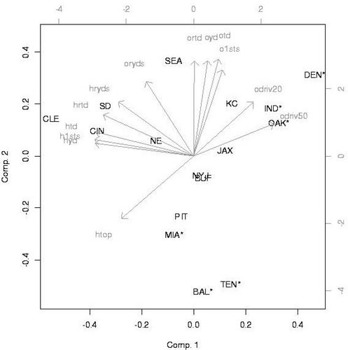
Our first attempt at the analysis involved only a few variables, because, at the time, these variables were the only ones available. Furthermore, we had information only for the American Football Conference (AFC; about half of the teams in the NFL). The first two principal components, given in explain almost 82% of the variation. The corresponding biplot (see, for example, Section 12.7 of CitationJohnson and Wichern 1998 or CitationVenables and Ripley 1997, pp. 388–389) from S-Plus® is given in , where the abbreviations for the variables used in the figure are given in and those for the teams are given in ; teams that made the playoffs are indicated by asterisks in the tables and figures. In order to avoid some confusion, we note that on , there is a counterintuitive correspondence between the points and the graph labels. The lighter axes (those on the upper and right-hand parts of the plot) correspond to the darker points (the team names), and vice-versa (see CitationVenables and Ripley 1997, p. 388).
Table 1. First Two Principal Components Using the American Football Conference (AFC) Data.
Table 2. Team Rankings Based on the Difference in the First Two Principal Components from for All Teams in the National Football League. Asterisks (*) denote teams that made the NFL 2000 playoffs.
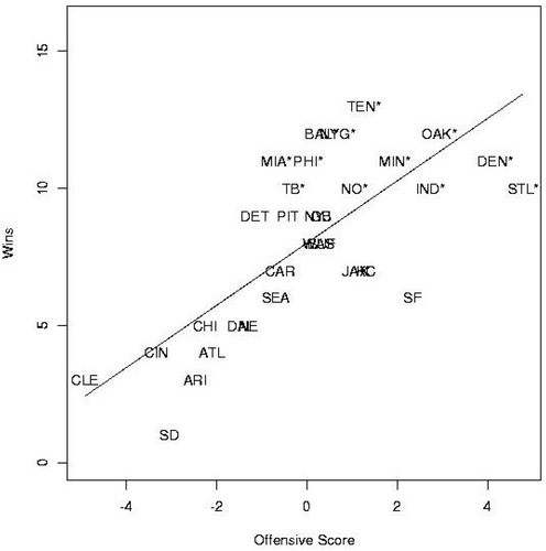
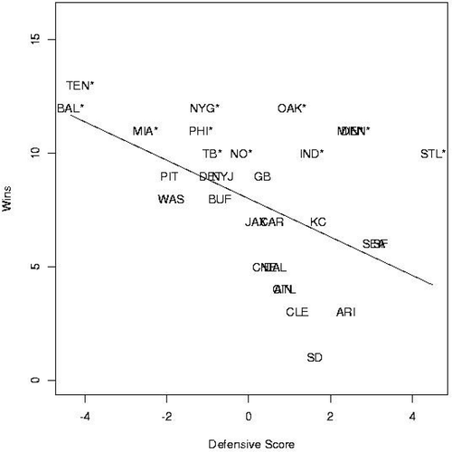
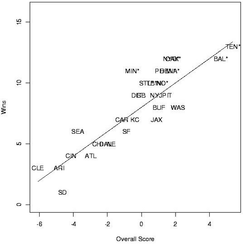
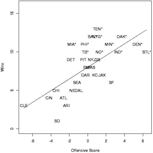
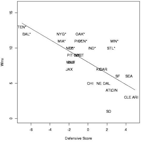
We interpret the first principal component as an “offensive score,” summarizing a team's offensive capabilities. The second principal component may be interpreted as a “defensive score,” summarizing a team's defensive capabilities. In the case of the first principal component, a large positive score indicates a good offensive team (indicated by being further to the right in ); in the second, a large negative score indicates a good defensive team (indicated by being closer to the bottom in ). We regressed these two principal components on team win percentage; the marginal regressions are depicted in Figures and . The R2 was 83%. We also found that the regression coefficients were close to equal, though of opposite signs. In fact, a hypothesis test – see, for example, CitationSamaniego and Watnik (1997) – established that the difference between the two principal components, labeled “overall score” in and , showed no significant difference between the model with just the overall score and the two separate scores.
presents the offensive, defensive, and overall scores (as defined in the previous paragraph), using the first two principal components of , for every NFL team. The National Football Conference (NFC) teams in provide a kind of “validation” of the AFC model. Six of the top seven AFC teams, according to this scoring criterion, made the playoffs. While the best NFC team according to this measure, the Washington Redskins, did not make the playoffs, the next five NFC teams did. (This could be taken as an indication that the team's win-loss record was not up to the teams' performance and thus an explanation for the Redskins' late-season firing of their coach.) As the reader might notice throughout, the Minnesota Vikings fared poorly in almost every model while the Washington Redskins tended to be overrated by the models. Interestingly, though not surprisingly, the St. Louis Rams had the NFL's best offense and the worst defense according to our model. Three playoff-qualifying AFC teams, the Oakland Raiders, Denver Broncos, and Indianapolis Colts, had a similar, but not as dramatic, imbalance.
Our attempt at principal components for the above variables using all of the NFL teams was a success. However, lest students think that principal component analyses on any subset would work, our attempt using just the NFC teams was not successful. That is, the principal component analysis of NFC data was not amenable to the clear offensive and defensive interpretation as the analysis of the AFC data. We were obviously fortunate to have chosen the AFC as the conference whose data would be entered first.
We were also fortunate to have the principal components come out in such a desirable (for us) way. As the reader will see shortly, when all (or most) of the variables are included in the analysis, the principal components method tends to look directly at the difference between the “home” and “opp” measures. This leads us to believe that the imbalance in the variables in this model is what caused these interpretable components.
4. Analysis of the Full Dataset
Of course, principal components can handle a much larger number of variables. There is no reason for us not to use every variable at our disposal. For the AFC only, the first principal component, contained in , explained only 29% of the variation. Nonetheless, this principal component, in our opinion, is a direct measurement of the team against its opponents. Namely, this principal component almost always subtracts the contribution of the opposing team from the corresponding contribution of its team for the offense and vice-versa for the defense.
Table 3. First Principal Components for the AFC Data Using All Variables.
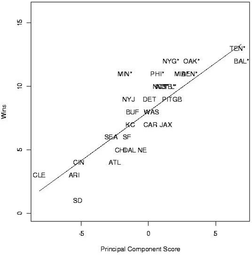
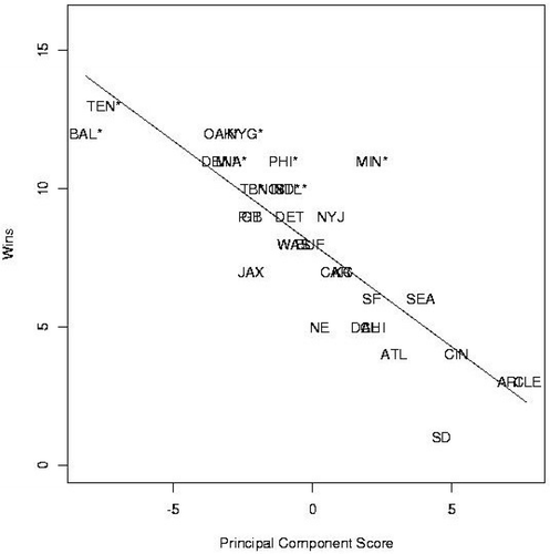
Using just that principal component, the regression on winning percentage for AFC teams provided an R2 of 72%. In and , we show how the principal components matched with the teams' number of wins. Again, we used the NFC as a “validation” group. The top five AFC teams, according to this criterion, made the playoffs. Five of the top six NFC teams made the playoffs.
Table 4. Team Rankings Based on the First Principal Component from for All Teams in the NFL. Asterisks (*) Denote Teams that Made the NFL 2000 Playoffs.
The first principal component, given in for the entire dataset (including all of the variables and all of the teams) explained only 21% of the variation. Again, as in , it appears to compare the team to its opponents directly.
Table 5. First Principal Components Using All Variables and All NFL Teams.
Table 6. Team Rankings Based on the First Principal Component from for All Teams in the NFL. Asterisks (*) Denote Teams that Made the NFL 2000 Playoffs.
The R2 for the regression of this principal component on the number of wins, as represented in , was 73%. Here, the top five AFC teams and five of the top six NFC teams made the playoffs. Furthermore, the principal component correctly selected the Super Bowl opponents and outcome, as well as all of the AFC playoff outcomes. (Its performance with respect to the NFC playoff match-ups was only successful half the time – the New York Giants' victories over the Philadelphia Eagles and the Minnesota Vikings and the New Orleans Saints' victory over the St. Louis Rams.)
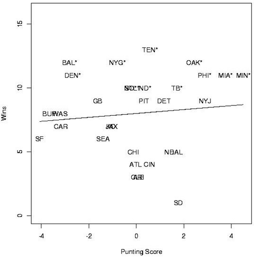
Finally, we summarize the data separately by offensive, defensive, and special teams variables. , , and present the relevant principal components. The first principal component for the offense explains 46% of the variation and the first principal component for the defense explains 49% of the variation. Note that the offensive principal component has very similar coefficients to the defensive principal component, with the obvious exception of time of possession. We feel that the difference between these two principal component scores gives an indication of overall team strength. In our attempt to summarize the special teams data, we found that considering the punting and kicking teams separately was superior to trying to do them both at once. Furthermore, we found that the ability of the punting team only had a significant effect on the number of wins. Thus the variables used in consist only of punting statistics. The first principal component in seems to represent the return capabilities of a team, though it only explains 22% of the variation. The second and third principal components appear most interpretable, summarizing the abilities of the home punting team and the opposing punting team. They explain 16% and 13% of the variation, respectively. We utilize these latter two principal components to devise a punting score in evaluating the teams.
Table 7. First Principal Component Summarizing Offensive Variables for Data from All NFL Teams.
Table 8. First Principal Component Summarizing Defensive Variables for Data from All NFL Teams.
Table 9. First Three Principal Components Summarizing Punting Variables for Data from All NFL Teams.
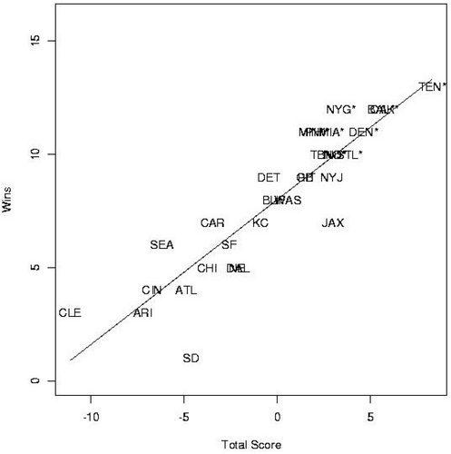
The “total score” in is computed as the offensive score (column 6 of the table and ) minus the defensive score (column 7 and ) plus one-half the punting score (column 8 and ). These weights were suggested from the regression of win percentage on all of these three scores. This regression had an R2 of 81%. Not surprisingly, the R2 for the regression of this “total score” (see ) on the number of wins was also 81%. Here, the top six NFC teams and the top five AFC teams made the playoffs. Interestingly, the Raiders and Jets punt teams push them up in the rankings. The Vikings, who have the best punting special team according to this analysis, also fair better. On the other hand, the Redskins are hurt by their punting team.
Table 10. Team rankings based on a summary of the offensive, defensive, and punting special teams play of each NFL team. The offensive and defensive principal components come from and . The punting summary measure consists of the difference of the second and third principal components from . The total score upon which the ranking is based consists of the offensive score minus the defensive score minus one-half the punting special teams score. Asterisks (*) denote teams that made the NFL 2000 playoffs.
6. Other Uses
This dataset need not be limited to use in multivariate statistics courses. For example, one could discuss whether teams in the NFC score more touchdowns than teams in the AFC (and whether it is appropriate to use a two-sample t‐test for these data). There are innumerable regression models that could be explored as well, but, as part of that, an interesting discussion could result from pointing out that the assumption of independence of observations is not met in this situation. Many students will recognize that the problem is not with, say homeint and oppint, being related (though there is collinearity), but with the number of wins across the teams that violates the assumption.
7. Conclusion
We have provided a reasonably comprehensive dataset for the 2000 NFL regular season. Furthermore, we presented and summarized some of our exploratory analyses on it. We believe that the dataset would be in a good example for use in multivariate statistics courses.
8. Getting the Data
The file nfl2000.dat.txt contains the raw data. The file nfl2000.txt is a documentation file containing a brief description of the dataset.
UJSE_A_11910541_SM0001.html
Download HTML (70.7 KB)Acknowledgements
The authors wish to acknowledge the assistance of our colleagues, Robert Shumway and Alan Fenech, for their helpful comments on a primitive version of this paper. We also thank the Department Editor, Roger Johnson, and two anonymous referees for their suggestions, particularly with respect to the graphs they recommended.
References
- Anderson-Cook, C., Thornton, T., and Robles, R. (1997), “Measuring Hockey Powerplay and Penalty Killing Efficiency”, in Proceedings of the American Statistical Association Section on Statistics in Sports, Alexandria, VA: American Statistical Association, 11–14.
- Johnson, R. A., and Wichern, D. W. (1998), Applied Multivariate Statistical Analysis (4th ed.), Upper Saddle River, NJ: Prentice Hall.
- Samaniego, F. J., and Watnik, M. R. (1997), “The Separation Principle in Linear Regression,” Journal of Statistics Education [Online], 5 (3). (ww2.amstat.org/publications/jse/v5n3/samaniego.html)
- Venables, W. N., and Ripley, B. D. (1997), Modern Applied Statistics with S-PLUS (2nd ed.), New York: Springer Verlag.
Appendix
Key To Variables in nfl2000.dat.txt
All rate variables use the total time of possession, that is the average time of possession times the number of games, as the denominator.
Each variable is provided for both the team of interest and their opponents – the former will be prefixed by “home” and the latter will be prefixed by “opp.”
Also included in this data set, but not used in the corresponding paper are longest kickoff return (kolong), number of points (points), rate of first downs (1rate), and turnover rate (torate = number of interceptions plus number of fumble recoveries, divided by time of possession). Columns Variable Description 1 - 3 initials team initials 5 - 26 team name and location of the team 28 - 29 wins wins 31 - 32 losses losses 34 - 35 homedrives50 drives begun in opponents' territory 37 - 38 homedrives20 drives begun within 20 yards of the goal 40 - 41 oppdrives50 opponents drives begun in team's territory 43 oppdrives20 opponents drives begun within 20 yards of goal 45 homepuntblock punts blocked by team 47 opppuntblock punts team had blocked 49 - 50 hometouch touchdowns scored by team 52 - 53 opptouch touchdowns scored against team 55 - 58 homeyards total yardage gained by offense 60 - 63 oppyards total yardage allowed by defense 65 - 68 hometop time of possession by offense (in minutes) 70 - 73 opptop time of possession by opponents' offense 75 - 76 homefgm field goals made 78 - 79 oppfgm field goals allowed to opponents 81 - 82 homefga field goals attempted 84 - 85 oppfga field goals attempted by opponents 87 - 89 opppuntno punts made by opponents 91 - 94 opppuntave average length of punts made by opponents 96 - 99 opppuntnet average change in field position during opponents' punts 101 – 102 opppunttb opponents' punts taken for touchbacks 104 – 105 opppunt20 opponents' punts that resulted in the team's offense beginning within 20 yards of their own (defensive) goal line 107 – 108 opppuntlong longest opponents' punt 110 – 112 homepuntno punts made by team 114 – 117 homepuntave average length of punts made by team 119 – 122 homepuntnet average change in field position during team's punts 124 – 125 homepunttb team's punts taken for touchbacks 127 – 128 homepunt20 team's punts that resulted in the opponents' offense beginning within 20 yards of their own (defensive) goal line 130 – 131 homepuntlong longest team punt 133 – 135 home1sts first downs obtained by offense 137 – 139 opp1sts first downs allowed by defense 141 – 142 homesacks sacks achieved by team's defense 144 – 145 oppsacks sacks allowed by team's offense 147 – 148 homekos kickoffs made by team 150 – 151 oppkos kickoffs received by team 153 – 156 homekoyds yards gained during kickoff returns 158 – 161 oppkoyds yards allowed to opposition during kickoff returns 163 – 166 homekoave average yards gained during kickoff returns 168 – 171 oppkoave average yards allowed during kickoff returns 173 – 175 homekolong longest kickoff return made by team 177 – 179 oppkolong longest kickoff return allowed by team 181 homekotds kickoffs returned for a touchdown by team 183 oppkotds kickoffs returned for touchdown by opposition 185 – 186 homerets punts returned by team 188 – 189 opprets punts returned by opposition 191 – 192 homefc punts “fair caught” by team 194 – 195 oppfc punts “fair caught” by opposition 197 – 199 homeretyds return yardage on punts by team 201 – 203 oppretyds return yardage on punts by opposition 205 – 208 homeretave average length of punt returns by team 210 – 213 oppretave average length of punt returns by opposition 215 homerettds punts returned by team for a touchdown 217 opprettds punts returned by opponents for a touchdown 219 – 220 homeint interceptions made by team's defense 222 – 223 oppint interceptions made against team's offense 225 – 226 homerecover fumbles recovered by team's defense 228 – 229 opprecover fumbles recovered by opposing defenses 231 – 232 numgames games played by team 234 – 237 opprateyds average number of yards gained per minute of possession by opponents 239 – 242 homerateyds average number of yards gained per minute of possession by team 244 – 247 opppuntrate average number of punts per minute of possession by opponents 249 – 252 homepuntrate average number of punts per minute of possession by team 254 – 258 oppratetd average number of touchdowns per minute of possession by opponents 260 – 264 homeratetd average number of touchdowns per minute of possession by team 266 – 269 winpercent winning percentage 271 – 275 hometorate turnovers obtained by team, per minute of possession by opponents 277 – 281 opptorate turnovers allowed by team, per minute of possession 283 – 286 home1rate first downs obtained by team, per minute of possession 288 – 291 opp1rate first downs allowed by team's defense, per minute of possession by opposition 293 – 295 homepoints points scored by team 297 – 299 opppoints points scored against team 301 – 303 conference conference to which the team belongs (AFC or NFC)
