A Computer Evolution in Teaching Undergraduate Time Series

Abstract

In teaching undergraduate time series courses, we have used a mixture of various statistical packages. We have finally been able to teach all of the applied concepts within one statistical package; R. This article describes the process that we use to conduct a thorough analysis of a time series. An example with a data set is provided. We compare these results to an identical analysis performed on Minitab.

• Statistical packages
• Time series analysis

1. Introduction

In a typical undergraduate time series class, we spend a considerable amount of time discussing analysis via multiplicative decomposition and Box-Jenkins models. Over the years, we have used various computer packages and programs to illustrate the analysis cycle. Until recently, we could never do all of these calculations in one package. We might use a combination of SAS and FORTRAN programs, or a combination of Excel, FORTRAN, and SAS. Now we can use just one statistical package, R, to produce all of the preliminary plots, transformations, decompositions, Box-Jenkins models, and forecasts.

The R langauage is is extension of a language called S, which was developed in the mid 1980s at then-Bell Labs. S was originally developed for use on UNIX mainframe systems. The language is similar to the C programming language. As S evolved, there became a need for a version for personal computers. The Mathsoft Corporation (now Insightful Corporation) produced Windows and Mac based versions called S-Plus. Finally, Ihaka and Gentleman (1996) put together a free ware version of S/S-Plus that they called R.

The help facilities within R are impressive. There are manuals available online, along with documentation for functions (R Development Core Team 2003). One of the manuals is “An Introduction to R” (Venables, Smith, and the R Core Development Team 2003) which has a tutorial. Finally, there is a search engine to find existing functions. We use that feature quite often when looking for a function name. This feature allows a user to enter a phrase into the engine. Options are revealed that contain the phrase.

There are many excellent books for S and S-Plus, and nearly all of these are appropriate for R users. For beginning users, the original S book by Becker, Chambers and Wilks (1988) is still quite useful. Also, the books by Spector (1994), and Krause and Olsen (2000) contain tutorials for novices. The classic Modern Applied Statistics with S, by Venables and Ripley (2002) shows both beginners and seasoned users needed skills in tandem with statistical constructs. There are many other books available for advanced programming and statistical modeling, such as Venables and Ripley (2000); Chambers and Hastie (1992); Chambers (1998), Pinheiro and Bates (2000), and Zivot and Wang (2002).

There are now a few books developed in conjunction with R. Dalgaard (2002) has a book for introductory statistics, and he does not assume any familiarity with the language. Fox (2002) has written a book for applied regression with both S-Plus and R.

The major advantages of R are quite easy to see. The first, and most meaningful, is that R is free. It can be downloaded from the Internet at any time from several locations around the world. The site that we typically use is lib.stat.cmu.edu/R/CRAN, which is at the Statistics Department at Carnegie Mellon University. There is a list of mirror sites at this location.

Next, R has a fast learning curve. We have used this package in our time series class as well as other upper level classes, and the students acquire the skills needed to manipulate R readily. We present a tutorial during the first class session, and assign problems. These problems let the student learn about existing capabilities initially. As the students learn the R nomenclature, they are also given functions to write themselves. After one or two sessions, they feel very comfortable with this package. They learn to write their own functions in order to eliminate repetitive tasks (and to impress their classmates).

Finally, R has impressive graphics capabilities. Not only do the graphs appear beautifully on the screen, they are easily saved in the proper formats for reports or Power Point presentations.

The students can use these functions to do a full analysis on their own data set. Part of the course grade depends on an extensive data analysis project. The students must select a topic, investigate its history, and produce an analysis of past behavior along with forecasts of future behavior. Often, students select stock price data for a particular company. They must do research on that company, while considering world events during the same time frame as the series. The students are frequently surprised at the role that a company might have played in the global market over time. Finally, they run the time series procedures and make forecasts. They can then determine which method yielded the best forecasts. Students have an appreciation of the model building process on real data, combined with user-friendly software.

In this paper, we will show the necessary processes in the development of a good time series analysis. Section 2 is devoted to the data preparation and input stage. Also, we stress the need for graphics. In Section 3, we discuss transformations and the commands for those transformations. Section 4 shows the multiplicative forecasting procedure. In Section 5, we present the Box-Jenkins analysis. We use a real data set for our analysis in Section 6. In Sections 2 − 6, all of our material is shown via the R program. We present a comparison between R and Minitab in Section 7. We would like to demonstrate that for undergraduate time series, R will be the package of choice. R gives the instructor options for more sophisticated material. Finally, in Section 8, we finish with a brief conclusion.

2. Initial Data Set-Up and Plots

When students bring their data sets, they enter them as numeric vectors, but then they change them to time series in the following fashion:

This command sets up a time series, y.ts, which is a monthly series that begins in January, 1997. Data must be converted to a time series object for some of the functions.

We used most of the data for the model building purposes, but left a few data points out at the end of the series for comparison for forecasting. A common example is the selection of a data set which ran from January, 1990, to December, 2001. Then January, February, and March were set aside as “actuals” for the forecast comparisons.

Once a time series is ready, we need to see a plot of the data. But that command is quite simple:

This will produce a time series plot with the observed values of y.ts on the vertical axis, and the time component on the horizontal axis. By converting to a time series object, the plot command extracts the time component automatically and produces a line chart.

With tremendous computing speed so freely available, students are occasionally tempted to omit the plotting step. However, we insist on viewing a plot of the data. Often, simply looking at the graph of the observed values can give insight in terms of historical events.

We saw an interesting example from looking at the Bank of America Monthly Closing Stock Price, as shown below.

Figure 1. Bank of America monthly closing stock price

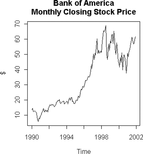
The recession in the early 1990s appears immediately, in which the business cycle trough occurs in March 1991. The crash of the Asian markets and the financial difficulties in the US markets in late 1997 and 1998 are readily apparent. The recent economic slowdown with its fluctuations finishes the picture. Students were then motivated to investigate some of these events, including Russia's default on its international debt, and incorporate them into their own projects.

3. Transformations

We are concerned with nonstationarity in time series, along with variance stabilization. We use the method as described in Box and Cox (1964):

At first glance, this formula seems quite formidable. Originally, we had our own function to derive this. But during the last semester, we found a more efficient function from Venables and Ripley (2002) in the MASS library which is a part of the R package. Here are the commands:

> #This command attaches the MASS library, which contains the Box-Cox command

> library(MASS)

> #We set up a sequence

> t1 <- 1:length(y.ts)

> #We create a linear model

> y.lm <- lm(y.ts∼t1)

> #We run the Box-Cox process

> boxcox(y.lm,plotit=T)

We first load the MASS library. Then we must construct a linear model object. This object is essentially a least squares regression model:

where the ε₂ are Gaussian white noise random variable with mean zero, and a variance . The boxcox function calculates the log-likelihood of the residual sum of squares (part of the variance estimate) for various values of the λ parameters. The goal is to maximize the log-likelihood function. Then we select the value of λ at that maximum to use as our transformation parameter.

The boxcox command as shown above uses −2 ≤ λ ≤ 2, in increments of 0.1. Also, the plot of the log-likelihood vs. λ is shown. We will iterate with finer gradations for λ until the differences between successive log-likelihood values are negligible.

Once the λ value is selected, we must perform the necessary transformation on the time series. We wrote a function, trans1, to complete this calculation. An example might appear as:

> y16.ts <- trans1(y.ts,0.16)

The y16.ts is a time series object which contains the transformed values.

4. Multiplicative Decomposition and Forecasting

Once the data have been plotted and transformed, we can begin the modeling process in depth. For the multiplicative decomposition method, we have the following equation:

where y_t is the observed value of the time series at time t, T_t is the trend factor at time t, S_t is the seasonal factor at time t, C_t is the cyclical factor at time t, and I_t is the irregular factor at time t. This method is described in some detail in Bowerman and O'Connell (1993) and Kvanli, Pavur, and Guynes (2000).

This process is designed for annual, quarterly, and monthly data sets. There must be a minimum of 3 years of data, regardless of the frequency. If annual data is used, the seasonal component is set to 1 for all values. When the seasonal component is requested, and the data frequency is not 1, the number of data points must be a multiple of the frequency. For instance, if monthly data is used, then the total number of data points must be a multiple of 12. The data can start at any time of the year, but the number of data points must maintain the annual integrity. However, if the seasonal component is not required, then the number of data points is arbitrary.

We have written our own function for the decomposition process, decom1. Here again, we exploit the time series object within the function. The only required input to the function is the name of the time series object. An optional input is an indication if the seasonal component is required. The default value is 1, which means that the seasonal values are requested.

The function returns a list of outputs. These include the deseasonalized values of the series, the trend values, the seasonal values, the cyclical values, and the irregular values. For monthly and quarterly data, an abbreviated list of the seasonal factors is produced as well. Also, the slope and intercept terms are shown as part of the trend calculation. Finally, if forecasts are requested, the function produces predicted values, and 95% prediction intervals for those values. We use the method suggested by Bowerman and O'Connell (1993) to produce the prediction intervals. If we had a time series, y16.ts, and we needed a 3 period forecast, the function would appear as:

Once the forecast values have been obtained, we can restore them to the original order of magnitude by using the trans1 function again. If the transformation parameter was 0.16, we can enter (1/.16), to return the forecasts and the upper and lower prediction levels.

Finally, we can determine the accuracy of the forecast. We created a function, forerr, that uses the actual data and the forecast values to calculate the mean absolute devation and the mean square error. Statements for this function appear in the Appendix. The command would appear as:

We will repeat this process with the Box-Jenkins method, and ascertain if one method outperforms the other.

5. The Box-Jenkins Approach and Forecasting

Many books have been written on the elegant Box-Jenkins (Box and Jenkins 1976) methodology and these procedures are wonderful to teach. With the aid of powerful computers, the equations can be appreciated by all students. We will consider the basic autoregressive integrated moving average model:

where is the autoregressive polynomial of order p, (1-B)^d is the differencing operator, is the moving average polynomial of order q, and the a_t are a Gaussian white noise sequence with mean zero and a variance and the y_t are the series values. The B is the backshift operator such that B^j y_t = y_t-j. We expand the autoregressive polynomial:

such that all of the roots of the polynomial are outside of the unit circle. Similarly, we can expand the moving average polynomial such that:

where all of the roots of the moving average polynomial are outside of the unit circle. We also assume that the autoregressive and moving average polynomials have no roots in common. Finally, the (1 – B)^d polynomial reflects the order of differencing needed to achieve stationarity. Such an expression is referred to as an autoregressive integrated moving average model, or ARIMA(p,d,q) model.

There is a library in R called ts which contains the arima function that will estimate the parameters of the ARIMA(p,d,q) model. The students test several models, and select the model which has the minimum value of the Akaike Information Criterion (AIC). In real world data, we must be concerned with problems of stationarity and differencing. We experiment with several levels of differencing in order to get seasonal values for our autoregressive parameters. For an ARIMA(1,1,1) model, the command would appear as:

• > #We attach the ts(Time Series) library

• > library(ts)

• > #This is the command for ARIMA models

• > arima(y16.ts,order=c(1,1,1))

As we found in the previous section, seasonal factors can play a major role in the model building process. Fortunately, there are seasonal (SARIMA) models that can be constructed:

with the usual assumption about roots outside of the unit circle. The (1- B^s)^D is the order of seasonal differencing. The notation for these models is ARIMA(p,d,q) × (P,D,Q)_s, in which P is the order of the seasonal AR polynomial, D is the order of seasonal differencing, Q is the order of the seasonal MA polynomial, and s is the seasonal period. We found these models to be extremely effective in our learning process. For a test ARIMA(1,1,1) × (1,1,1)₁₂ model, the command would be:

• > arima(y16.ts,order=c(1,1,1),seasonal=list(order=c(1,1,1),period=12))

Once the appropriate model has been selected, an object must be saved to pass to the prediction function. If the previous model is selected, the command would appear as:

• > y16.lm <- arima(y16.ts,order=c(1,1,1),seasonal=list(order=c(1,1,1),period=12))

Next, R has its own prediction function for time series objects, which is predict.Arima. Here is a sample of the command, with a 3 period forecast:

• > predict.Arima(y16.lm,n.ahead=3)

We calculate our own intervals, as the predict.Arima command returns the predictions and the standard errors. These intervals are merely ± 1.96 se for each predicted value, where se is the standard error.

Finally, we transform the predicted data back to its original form with the help of trans1, and run the error comparison via forerr. The students can then make an informed decision on which model provides the most meaningful forecasts.

6. An Example

We downloaded closing stock prices from the Home Depot Corporation. These data can be found at www.yahoo.com. We have monthly data from January, 1985 until December, 2001. We kept the January through March 2002 data separate for forecasting comparisons. Here are the set-up commands:

• > #We take a data vector and make it a time series object

• > y.ts <- ts(hd1,start=c(1985,1),frequency=12)

• > #We put the Jan – Mar data into its own time series object

• > ya.ts <- ts(c(49.98,49.89,48.55),start=c(2002,1),frequency=12)

We will use the ya.ts later in the process. The y.ts series is the necessary time series object. We now consider a plot of the historical data:

• > plot(y.ts,ylab=“$”,main=“Home Depot Monthly\nClosing Stock Price”)

Figure 2. Home Depot monthly clossing stock price.

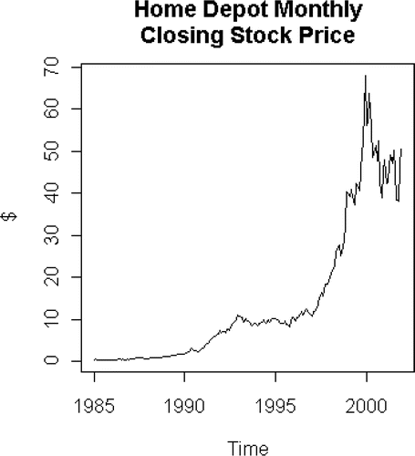
We see the not unexpected patterns; the fluctuations of the market in the late 1990s, and the serious downturn in the late part of 2001. Now we must check to determine if a transformation is needed:

• > library(MASS)

• > t1 <- 1:length(y.ts)

• > yhd.lm <- lm(y.ts ∼ t1)

• > boxcox(yhd.lm,plotit=T)

Figure 3. Finding λ for the Box-Cox transformation.

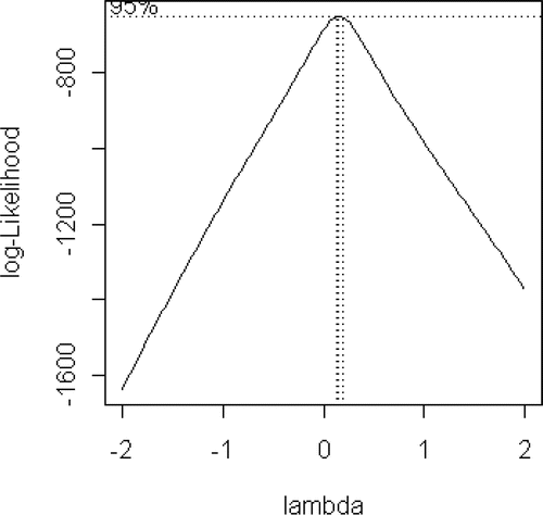
After a bit more fine-tuning, we find that the λ = 0.16. To produce the transformed series, we use:

• > #After we determine the proper lambda value, we transform the series

• > y16.ts <- trans1(y.ts,0.16)

Now we can turn to the multiplicative decomposition method. We return to the decom1 method:

• > #We run the mult. decomposition function on the transformed data

• > y16d <- decom1(y16.ts,fore1=3)

• > #These are the predictions and confidence intervals for the transformed data

• > y16d$pred

Table

1	2	3
1.920953	1.933335	1.948505

> y16d$predlow

Table

1	2	3
1.790454	1.802817	1.817969

> y16d$predup

Table

1	2	3
2.051452	2.063852	2.079041

We only reproduced the prediction values and intervals here. More of the y16d object appears in the Appendix. We will reverse the transformation procedure to return the forecast values to the correct order of magnitude:

• > #We return our forecasts back to the original order

• > y16u <- trans1(y16d$pred,(1/0.16))

• > y16u

Table

1	2	3
59.15335	61.57712	64.65985

• > #We return the intervals back

• > trans1(y16d$predlow,(1/0.16)

Table

1	2	3
38.10832	39.78309	41.91942

> trans1(y16d$predup,(1/0.16))

Table

1	2	3
89.20372	92.62781	96.97159

Finally, we would like to have some measures of accuracy for our forecasts. We will use the forerr function as follows:

• > #We calculate MAD, MSE on Forecasts

• > forerr(ya.ts,y16u)

• $mad

• [1] 12.32344

• $mse

• [1] 160.0887

We will compare these measures to those produced by the Box-Jenkins method to determine the best fit for this particular data set.

Here is a table with the actual values, the forecast values, and the intervals for January through March of 2002. As we can see, the actual values are decreasing, while the forecasts are increasing. The intervals are quite wide, and would not be of great value to a trader.

Table 1. Multiplicative Decomposition Forecasts

Date	Actual	Forecast	Lower Bound	Upper Bound
Jan	49.98	59.15	38.11	89.20
Feb	49.89	61.58	39.78	92.63
Mar	48.55	64.66	41.92	96.97

We always begin the Box-Jenkins method by checking for an AR(1) model:

• > library(ts)

• > #We run different ARIMA/SARIMA models on the transformed data

• > #We select the best model based on the minimum AIC

• > arima(y16.ts,order=c(1,0,0))

• > arima(y16.ts,order=c(1,1,0))

• > arima(y16.ts,order=c(1,1,1))

• > arima(y16.ts,order=c(2,1,0))

• > arima(y16.ts,order=c(2,1,1))

• > y161.lm <- arima(y16.ts,order=c(1,1,1))

• > y161s.lm <- arima(y16.ts,order=c(1,1,1),seasonal=list(order=c(1,1,1),period=12))

We sometimes use both the ARIMA and SARIMA models, simply for extra practice. The models that we have obtained are ARIMA(1,1,1) and ARIMA(1,1,1) × (1,1,1)₁₂, respectively. The equations would be:

We obtain forecasts from each model as:

• > y161p <- predict.Arima(y161.lm,n.ahead=3)

• > #Regular ARIMA – calculate Forecast and se for transformed data

• > y161p

• $pred

Table

	Jan	Feb	Mar
2002	1.871792	1.874719	1.872248

$se

Table

	Jan	Feb	Mar
2002	0.02069411	0.03057785	0.03708152

• > y161pl <- y161p$pred – 1.96*y161p$se

• > y161pu <- y161p$pred + 1.96*y161p$se

• > y161s <- predict.Arima(y161s.lm,n.ahead=3)

• > #Seasonal ARIMA – calculate Forecast and se for transformed data

• > y161s

• $pred

Table

	Jan	Feb	Mar
2002	1.869099	1.869018	1.880240

$se

Table

	Jan	Feb	Mar
2002	0.02067993	0.02889495	0.03515230

• > y161sl <- y161s$pred – 1.96*y161s$se

• > y161su <- y161s$pred + 1.96*y161s$se

We must undo the transformation for each Box-Jenkins model:

• > #Regular ARIMA – return to original data

• > y161u <- trans1(y161p$pred,(1/0.16))

• > #Forecasts

• > y161u

Table

	Jan	Feb	Mar
2002	50.30490	50.79854	50.38148

• > #Lower limit for CI

• > trans1(y161pl,(1/0.16))

Table

	Jan	Feb	Mar
2002	43.86780	41.46290	39.33705

• > #Upper limit for CI

• > trans1(y161pu,(1/0.16))

Table

	Jan	Feb	Mar
2002	57.51750	61.83970	63.92145

• > #Seasonal ARIMA – return to original data

• > y161uu <- trans1(y161s$pred,(1/0.16))

• > #Forecasts

• > y161uu

Table

	Jan	Feb	Mar
2002	49.85414	49.84070	51.74074

• > #Lower limit for CI

• > trans1(y161sl,(1/0.16))

Table

	Jan	Feb	Mar
2002	43.47017	41.12099	40.97337

• > #Upper limit for CI

• > trans1(y161su,(1/0.16))

Table

	Jan	Feb	Mar
2002	57.00781	60.06359	64.79127

Finally, we calculate the error measures for each model:

• > #Regular ARIMA

• > forerr(ya.ts,y161u)

• $mad

• [1] 1.021643

• $mse

• [1] 1.428448

• > #Seasonal ARIMA

• > forerr(ya.ts,y161uu)

• $mad

• [1] 1.121969

• $mse

• [1] 3.399703

Here are the tables with the actual values, the forecast values, and the intervals for January through March of 2002 for each of the Box-Jenkins models. For the regular ARIMA, the intervals are considerably more narrow. The March forecast value decreases, which matches the pattern of the actual value. In the second table, the SARIMA model is excellent in the first two months, but is disappointing in March. We see narrow intervals yet again, which can provide useful information to real-world investors.

Table 2. Regular ARIMA Forecasts

Date	Actual	Forecast	Lower Bound	Upper Bound
Jan	49.98	50.30	43.87	57.52
Feb	49.89	50.80	41.46	61.84
Mar	48.55	50.38	39.34	63.92

Table 3. Seasonal ARIMA Forecasts

Date	Actual	Forecast	Lower Bound	Upper Bound
Jan	49.98	49.85	43.47	57.01
Feb	49.89	49.84	41.12	60.06
Mar	48.55	51.74	40.97	64.79

The Box-Jenkins models far outperform the multiplicative decomposition method. In all of the ARIMA models, the MAD and MSE values are less than 5, while the other method struggles. For the best model in the Box-Jenkins, we would go with the regular ARIMA for the full 3 month period. The SARIMA was most impressive in January and February, but the upward blip in March disturbed the performance. Overall, however, we can see for this data set, that the Box-Jenkins methods are the most effective.

7. Minitab Comparison

We used the same data set with the Minitab program. Minitab is used in several of our references. A 30-day demonstration version is available for free downloading from www.minitab.com. Even though we had not used Minitab in several years, we found the processes that we needed easily, with the aid of the online help files. We wil use the Box-Cox transformation, the multiplicative decomposition, and the ARIMA process.

The Box-Cox transformation is located on the Control charts menu. Here we came upon an interesting divergence. The optimal λ was found to be 0.113, which is different from that found in R. We use both the 0.113 transformed series and calculated a 0.16 transformed series, simply for comparison purposes.

On the time series menu, we used the decomposition option. We used the trend and seasonal option. We noted that there were no options for cyclical and irregular components. We produced the forecast values for each series. There is also no option for confidence interval. We were not entirely surprised by this, because the confidence intervals described by Bowerman and O'Connell (1993) is an empirical method rather than a theoretical one. When we transformed the forecasts back, our decomposition values were quite removed from the actuals. Using the 0.113 transformed series, we found a MAD value of 17.3767, and a MSE value of 313.2327. With the 0.16 transformed series, we obtained a MAD value of 12.2967, with a MSE of 160.5583. The 0.16 series has values comparable to those calculated by R.

For the ARIMA functions, the menu is quite easy to use. The forecasts are calculated by an option on the menu. We did notice that the AIC is not available. We use the AIC to determine the best model, so this could be a potential problem. For forecast errors, the regular ARIMA(1,1,1) yielded a 1.40 MAD value and a MSE value of 3.3006 for the 0.113 series, while the 0.16 series yielded a 1.4067 MAD with a 4.3843 MSE. Finally, the seasonal model produced a MAD 2.5967 with a MSE 8.2023 for the 0.113 series. The 0.16 series had a MAD of 1.0133 and a MSE of 1.4122. Here again, the 0.16 results are in line with those from R.

Our comparison study is quite interesting. We really do have a mixture of results. For ease of use, Minitab would be the winner. It is menu driven, and students are accustomed to that scenario. Students are familiar with worksheet functions. Minitab, too, also has beautiful plots that can be put into other packages. However, we did see more accurate forecasting results with the R package. We obtained quite different results for the transformation, which impacted the rest of the process. The main concern was the lack of the AIC. This statistic is much more effective than looking at autocorrelation functions.

The R package has extensions for more advanced time series methods. There are functions to generate simulated ARIMA series for students to practice model identification. Large scale simulation studies can be carried out easily via the R BATCH command. Many of the standard time series data sets, such as the Canadian lynx data, and sunspot data are part of the R package. Also, data sets from both SAS and SPSS can be imported into R. Minitab supports SPSS but not SAS data files. Topics such as the Kalman filter, fractional differencing and the ARCH/GARCH models are available in R, but not in Minitab.

A final consideration may be the intended audience for the course. If the students do not have extensive computer experience, Minitab may be preferable. For more sophisticated users, R may be the language of choice.

8. Conclusion

In a comparison with Minitab and R, we should consider cost and ease of use. If students do not have access to Minitab on campus, they can “rent” it for a semester. Minitab is user-friendly and menu driven. At many universities, the cost factor is not a problem, since most packages are supported in computer labs. But with budget constraints, smaller universities can still have access to an excellent statistics package.

We have found that the students learned and enjoyed their time series course by the concentration on one software package. Since R is free and is easily downloaded, students do not need to be concerned with access. With only one package to learn, we could spend more time refining concepts, and developing better models. Also, we could use both regular and seasonal models to their full advantages. The R package is a most effective learning tool for the undergraduate time series experience. We can employ R for concepts at all levels to supplement students' knowledge base.

Acknowledgements

The authors wishes to thank the editor and two referees for their very helpful comments and suggestions.

Appendix

Here is the source code for the R functions that we wrote:

> trans1 function(x,lam=1) { p1 <- abs(lam) #Check for negative values if(min(x) <=0 && p1 != Inf)stop("Data values must be positive") n1 <- length(x) wa <- numeric(length=n1) #Set up for exp if(p1 == Inf) { wa <- exp(x) return(wa) } #Set up for log if(p1 == 0) { wa <- log(x) } #Set up for regular power else { wa <- exp(p1*log(x)) } #Set up for negative power if(lam < 0)wa <- 1/wa return(wa) } > decom1 function(x,fore1=0,se1=1) { if(is.ts(x) != T)stop("Data must be a time series") n1 <- length(x) f1 <- tsp(x)[3] f21 <- f1 ck1 <- n1/f1 if(se1 != 1)f21 <- 1 if(ck1 != floor(ck1))stop("Need exact values for a year") if(fore1 < 0)stop("Forecast value must be positive") if(fore1 > n1)stop("Forecast value must be less than series length") #Load ts library library(ts) #Now start the seasonal process #This is NOT done for annual data if(f21 != 1) { y <- filter(x,rep(1,f1))/f1 z <- filter(y,rep(1,2))/2 xx <- as.vector(z) z1 <- c(NA,xx[-n1]) w1 <- x/z1 w2 <- matrix(w1,nrow=f1) w3 <- apply(w2,1,function(x)mean(x,na.rm=T)) w4 <- sum(w3)/f1 w3 <- w3/w4 sea1 <- rep(w3,length=n1) sea1 <- ts(sea1,start=start(x),freq=f1) ab <- f1 - start(x)[2] +2 sea2 <- sea1[ab:(ab+f1-1)] dy <- x/sea1 } else { sea1 <- rep(1,length=n1) sea2 <- 1 dy <- x } #Begin fitting the trend t1 <- 1:n1 trend.lm <- lm(dy ~ t1) #Obtain Final Fitted series yhat <- trend.lm$fitted.values*sea1 #We will get cyclical and irregular values cr1 <- x/yhat cy1 <- as.vector(filter(cr1,rep(1,3))/3) ir1 <- cr1/cy1 #Calculate forecasts if needed if(fore1 != 0) { new1 <- data.frame(t1=(n1+1):(n1+fore1)) pred1 <- predict(trend.lm,newdata=new1,interval="prediction") pred2 <- (pred1[,3] - pred1[,2])/2 xs1 <- sea1[1:fore1] pred4 <- pred1[,1]*xs1 pred5 <- pred4 - pred2 pred6 <- pred4 + pred2 zz <- list(int=trend.lm$coef[1],slope=trend.lm$coef[2],deas=dy, trend=trend.lm$fitted.values,seas=sea1,seay=sea2,cycle=cy1,irr=ir1, pred=pred4,predlow=pred5,predup=pred6) } else { zz <- list(int=trend.lm$coef[1],slope=trend.lm$coef[2],deas=dy, trend=trend.lm$fitted.values,seas=sea1,seay=sea2,cycle=cy1,irr=ir1) } zz } forerr function(act1,fore1) { #Check input lengths if(length(act1) != length(fore1))stop("Length of actual and forecast not equal") #Calculate Mean Absolute deviation mad1 <- sum(abs(act1-fore1))/length(act1) #Calculate Mean Square Error mse1 <- sum((act1-fore1)^2)/length(act1) zz <- list(mad=mad1,mse=mse1) return(zz) }

We will print a sample of the y16d object here:

> y16d $int (Intercept) 0.7810098 $slope t1 0.005596328 . . . $pred

Table

1	2	3
1.920953	1.933335	1.948505

$predlow

Table

1	2	3
1.790454	1.802817	1.817969

$predup

Table

1	2	3
2.051452	2.063852	2.079041

References

- Becker, R.A., Chambers, J.M., and Wilks, A.R. (1988), The New S Language: A Programming Environment for Data Analysis and Graphics, Pacific Grove, CA: Wadsworth and Brooks Cole.
- Bowerman, B.L., and O'Connell, R.T. (1993), Forecasting and Time Series: An Applied Approach (3rd ed.), Pacific Grove, CA: Duxbury.
- Box, G.E.P., and Cox, D.R. (1964), “An analysis of transformations,” Journal of the Royal Statistical Society, Series B, 26, 211–252.
- Box, G.E.P., and Jenkins, G.M. (1976), Time Series Analysis: Forecasting and Control, San Francisco, CA: Holden-Day.
- Chambers, J.M. (1998), Programming with Data: A Guide to the S Language, New York: Springer.
- Chambers, J.M, and Hastie, T.J. (1992), Statistical Models in S, Pacific Grove, CA: Wadsworth and Brooks Cole.
- Dalgaard, P. (2002), Introductory Statistics with R, New York: Springer.
- Fox, J. (2002), An R and S-Plus Companion to Applied Regression, Thousand Oaks, CA: Sage Publications.
- Ihaka, R., and Gentleman, R. (1996), “R: A Language for Data Analysis and Graphics,” Journal of Computational and Graphical Statistics, 5, 299–314.
- Krause, A., and Olson, M. (2000), The Basics of S and S-Plus, New York: Springer.
- Kvanli, A.H., Pavur, R.J., and Guynes, C.S. (2000), Introduction to Business Statistics (5th ed.), Cincinnati, OH: South-Western.
- Pinheiro, J.C., and Bates, D.M. (2000), Mixed-Effects Models in S and S-Plus, New York: Springer.
- R Development Core Team (2003), R Environment for Statistical Computing and Graphics, CRAN.R-project.org/manuals.html
- Spector, P.C. (1994), An Introduction to S and S-Plus, Belmont, CA: Duxbury.
- Venables, W.N., and Ripley, B.D. (2000), S Programming, New York: Springer.
- Venables, W.N., and Ripley, B.D. (2002), Modern Applied Statistics with S-Plus (4th ed.), New York: Springer.
- Venables, W.N., Smith, D.M. and the R Development Core Team (2003), An Introduction to R, London: Network Theory Limited.
- Zivot, E., and Wang J. (2002), Modeling Financial Time Series With S-Plus, New York: Springer-Verlag.