Abstract
This article shows a concrete and easy recognizable view of a cumulative distribution function(cdf). Photograph views of the search tabs on dictionaries are used to increase students' understanding and facility with the concept of a cumulative distribution function. Projects for student investigations are also given. This motivation and view helps the cdf become a bit more tangible and understandable.
1. Introduction
Images of bar charts, histograms, stem-and-leaf diagrams, frequency distributions, and probability density functions can all be introduced and explained via an intuitive, constructive motivation. We imagine blocks, beads, or digits stacked or piled up in defined bins. For categorical data the bins are named categories in the data. The stacked up objects display the data as a bar chart. Higher stacks indicate the categories that appear more frequently. For continuous or discrete quantitative data, the stacks are built on bins that fall along a number line. For equal sized bins the height of a stack is proportional to f(x), the density or relative frequency of occurrence of numbers in a bin around the real number x.
Between these two extremes of named categories and the real number line, lie ordinal data. These are categorical data ordered in a logical or well accepted way. Ordinal data have long been illustrated with course grades (A, A-, B+, B, etc.) or levels of satisfaction or agreement (very strongly agree, strongly agree, etc.). The alphabet also provides a well understood ordering. A frequency distribution of the usage of letters can be represented in an alphabetically ordered bar chart. For example, a bar chart of the tiles in the crossword game of Scrabble shown in , roughly mirrors the occurrence of the letters used in the English language. The letter “E” is most frequent, with twelve occurrences out of 100 tiles, yielding a relative frequency of 0.12. This closely matches the occurrence of the letter “E” in English. Other letters such as “S” were deliberately underrepresented in the design of Scrabble. The relative frequency of “S” in English is about 0.063, but too many “S” letters in Scrabble would make it too easy to form the plurals of nouns used in the game. To make this less likely, the Scrabble “S” is represented with a relative frequency of only 0.04. Other letters are also underrepresented as shown in CitationRichardson et al. (2004).
Figure 1. A photograph of Scrabble letter tiles stacked to see their frequency distribution (not shown are two blank tiles)

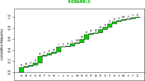
These images of frequency distributions seem natural and easily understandable. In contrast, the cumulative distribution function has been more difficult to visualize in a natural way. Given the frequency distribution f(x) for a discrete quantitative or ordinal variable, we define F(x) to be the cumulative relative frequency count of all measurements less than or equal to x. For the Scrabble example, × ε {A,B,C,…,Z}, and F(x) represents the cumulative relative frequency of all tiles with letters occurring at or before x. For example, if × = “E”, then F(“E”) is the cumulative count of the frequencies of all the letters “A”, “B”, “C”, “D”, “E” out of the 100 Scrabble tiles. That is, F(“E”) = 0.27, or, 27% of all Scrabble letters occur at or before the letter “E” in alphabetical order. The entire cumulative frequency distribution is shown in .
Figure 2. The cumulative distribution function for the letters in the Scrabble crossword board game.
To many students this construction of cumulative distribution functions (cdfs) seems artificial and more contrived than the simpler view of the frequency distribution. We are not as familiar with cumulative distribution functions because they do not occur routinely in much of our experience. Further it seems that work has to be done to convert a density function into a cdf. But for a continuous random variable, we know from probability that the cumulative distribution function is the more fundamental quantity. The frequency distribution is derived from the cdf through differentiation. But as it is presented in many elementary textbooks, we have to process the frequency distribution to produce the cdf. Thus even though mathematically we know it works in reverse, to some it seems that a cdf is a derivative of the density, in the literal meaning that the cdf must be derived from the frequency distribution. A cumulative distribution function does not appear to be the more fundamental idea from which a density function is derived.
It is the purpose of this article to provide instructors and students with a concrete and easy recognizable, visual example of cumulative distribution function (cdf).
2. A Dictionary Cumulative Distribution Function
shows a cumulative distribution function that can be seen and understood with relative ease. This is a side view of the pages of the paperback version of the Oxford Advanced Learners' Dictionary. Small colored squares for each letter are shown on the edge of each page. These colored squares act as tabs running from the top of the page for letters early in the alphabet to the bottom of the page for those letters that come later. These printed alphabetical marks on the edges of the pages help speed the look up of words and their definitions. This is really one of the first search engines.
When the dictionary is placed on its side, these colored tabs produce a cumulative distribution function for words from the English language. We have a visual and understandable image () of a cumulative distribution function. We can quantify this by noting, for example, that 93 pages of this dictionary are devoted to the letter “A”, so 93 pages have tabs colored to act as guide tabs to words starting with “A”. The last page number of each letter's tab indicates the number of pages devoted to words that begin with letters occurring, in alphabetical order, before that tab. Let G(x) denote the page number of this last page for each letter . These are the cumulative counts of pages for words beginning with each letter in the English alphabet, shown in . The maximum of G(x), call it M, is just the number of the last page of the dictionary for the letter “Z”. Define F(x) to be G(x)/M. Then F(x) represents the cumulative relative frequency of letters of the alphabet. This is the alphabet's cdf.
Table 1. Oxford Advanced Learners' Dictionary
Figure 3. A photographic side view of the Oxford Advanced Learners' Dictionary. Inserted below is a photo manipulation showing the frequency distribution of the dictionary's letters.
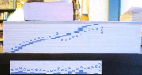
So what can we learn from and this table? The alphabet begins with a few large tab regions, rising vertically. This indicates that the first few letters of the alphabet begin many words. The middle of the alphabet is not so well represented. The letters of “I”, “J”, and “K” begin many fewer words with their collective contribution of colored tabs not extending vertically to any great extent. Big jumps at “P” and “S” indicate that many words start with those letters. They bracket a thin tab of very few words beginning with “Q”. The tail of the alphabet is so thin that the final three letters are combined into a single colored tab representing “X,Y, and Z” together.
The “S” tab spans the most pages, indicating more words in English start with “S” than with any other letter. From our consideration of Scrabble, recall that the letter “E” is most frequently occurring letter in English, but keep in mind that dictionary tabs consider only the first letters of words. As first letters, the letter “S” is most frequently occurring in English. From the table we can find the number of pages devoted to the letter “S”. This comes from subtracting G(“R”), which is the value that represents the cumulative count just prior to “S”, from G(“S”). This is G(“S”) — G(“R”) = 1558 — 1326 = 222 pages devoted to words that start with the letter “S”. We can divide these frequency counts by the maximum frequency count, M, resulting in relative frequency counts. Both frequency and relative frequency counts for each letter are also shown in . Photo manipulation software also allows us to visually collapse the cdf and place the tabs side-by-side to see the histogram of alphabetic frequencies, shown in the insert of . Here we can easily see that after the letter “S” is most frequently used and that the two next most frequent starting letters in English are “C” and “P”.
Of course what this shows is that more pages are devoted to the letter “S” than to the letter “K”, for example. This is most certainly because more English words start with “S” than “K”. But what about other pairs of letters, say “G” and “H”? Do more words start with “G” or more with “H”? Perhaps the definitions of the words starting with G are longer than those for “H”. This would give “G” more pages than “H” with perhaps fewer words. If we make the simplifying assumption that more pages mean more words, rather than more pages mean longer definitions, then the size of the letter tabs will be proportional to the frequency of words beginning with each letter of the alphabet.
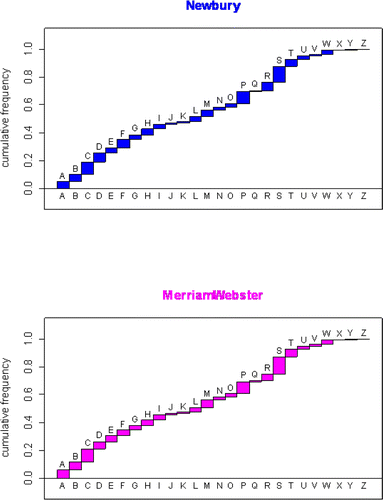
This image represents a snapshot of the words in the English language. We can quickly see which letters begin more words than others. This is, of course, just one dictionary. How reliable is this representation of the English language? I examined five other large dictionaries: CitationMicrosoft Encarta College (2001), CitationNew Oxford American (2001), CitationMerriam-Webster Collegiate (1998), CitationRandom House Webster's College (1995), and CitationNewbury House Dictionary of American English (1999). shows the cumulative counts for the smallest and largest of these English dictionaries: a small paperback edition (Newbury House) and a more comprehensive reference (Merriam-Webster Collegiate). Although minor editorial discretions are evident, the cdfs in are nearly identical. The cdfs for the others (not shown) are also nearly identical. A consensus image of the English language emerges from these cumulative functions since there is a great deal of common overlap for each dictionary.
Table 2. Cumulative frequencies (page numbers at the end of lettered tabs) of two English language dictionaries are shown along with cumulative relative frequencies.
Figure 4. Cumulative Relative Frequencies for the two English Language dictionaries shown in . Notice the near identical cdfs.
A formal test of the equality using the discrete Kolmogorov-Smirnov statistic can compare two dictionary cdfs. Let F(x) represent the cdf of the most comprehensive Merriam-Webster Collegiate dictionary. This will be taken as a standard. For another dictionary of n pages, let Hn(x) represent this other dictionary's cdf. The Kolmogorov-Smirnov statistic tests the null hypothesis that a sample cdf Hn(x) is equal to F(x). A statistic D = max n1/2 | H n(x) - F(x) | measures the discrepancy between two cdfs, where the maximum is taken over the 26 letters of the alphabet. The p-values for testing each of the cdfs of the English dictionaries discussed above were all greater than 0.57, indicating no significance difference.
3. Other Languages
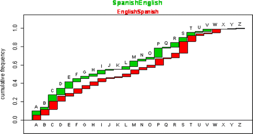
How does the English cumulative distribution function compare with other languages? is a side view of the Oxford Spanish Dictionary. The upper portion of the dictionary is for translating English into Spanish. It is another representation of the English cumulative distribution function that we saw earlier. Notice the second tab, for the letter “B”. The “B” tab extends halfway into “A” and also into “C”. The editors of this dictionary have not confined the tabs to each letter as before, but they have a larger extent of overlap spanning the letter positions on either side. Although the jumps from one letter to another remain correct, the inked contribution of each letter's tab is spread out over a range of neighboring letters resulting in a more connected and smoother cumulative distribution. The bottom portion of this dictionary is for translating Spanish into English. In this bottom portion, we have a similarly smoothed cumulative distribution function for Spanish. The most frequent first letter in Spanish is “C”. Notice how the Spanish cumulative distribution function builds up more rapidly than English early in the alphabet, only to have English include more frequent words starting with later letters. The cumulative counts are given in and a more precise plot in . The p-value for the discrete Kolmogorov-Smirnov statistic comparing the English and Spanish cdfs results in a p-value < 10−4, indicating a significant difference.
Table 3. Page numbers at the end of each lettered tab from the Oxford Spanish Dictionary
5. Student Investigations
Many investigations and exercises using dictionaries are available for student projects. CitationWarton (2007) describes several exercises connected with estimating the size of a student's vocabulary. Shown below are several other projects connected with using dictionaries and their tabs as cdfs.
How accurate is the assumption that we made earlier that more pages mean more words not longer definitions? Consider two letters say “G” and “H”. Students could select random samples of words beginning with each letter and then record the number of words in their definitions. Students could perform a t-test to answer the question: Is the mean definition length significantly different for the two letters?!
What editorial differences account for the minor differences in the English dictionaries? Consider two English dictionaries and two letters that do not have the same relative frequency of occurrence. What words are included/excluded from one compared to the other? Are the editors including more technical or colloquial words in one as opposed to the other?
Exercises for students could include comparing the dictionaries of other languages. For example, how similar are the cdfs for Spanish, Italian and Portuguese? Have students investigate a Hawaiian language dictionary. The Hawaiian language has only 12 letters. Its cdf looks markedly different from English.
Telephone directories also often have the same type tabs for quick name searches. Other investigations could include how do word cdfs from a dictionary compare with last name cdfs from a telephone directory?
How do the cdfs compare from special topic dictionaries, like medical or legal?
This book-tab concept can also serve as an analogy for students to understand the shapes of cumulative frequency distributions even for continuous random variables. For example, consider the cdf for a list of numbers having a Chi-square distribution with 3 degrees of freedom. Imagine tabs printed on the side of a large book of ordered numbers, perhaps rounded off to yield the image that we have created in .
Figure 7. Photographic illustration of the tabs on a hypothetical book of ordered Chi-square random observations with three degrees of freedom. The tabs indicate rounded values.
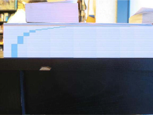
For low numbers, early in the book, the tabs are large indicating many pages devoted to those early numbers with many occurrences of numbers in a relatively small range. For higher numbers, later in the book, the tabs stretch out more horizontally indicating relatively few occurrences of many more individual numbers across a much wider range. This rapid build up and slow tapering off can then be easily understood to correspond to a list of numbers that is skewed to the right. If this were a language dictionary we would see almost all the words beginning with A, B, C, D with the later part of the alphabet only slightly represented. Similar analogies can be developed for other shaped distributions.
| 6. | How would the words look in a language whose tabs corresponded to a cdf of a symmetric, bell-shaped distribution? Or a U-shaped distribution? Or a left-skewed distribution? | ||||
6. Summary
A concrete and easy recognizable view of cumulative distribution functions has been presented. The reference tabs on pages of dictionaries present students with a visual and practical understanding of cumulative distribution functions. Instructors and students alike have a readily available cdf for projects and investigations. This view helps the cdf become a bit more tangible and understandable.
Acknowledgments
The author gratefully acknowledges the helpful comments and suggestions of the editors and the referees during the preparation of this manuscript.
References
- Merriam-Webster Collegiate Dictionary (1998), Springfield, MA: Merriam-Webster.
- Microsoft Encarta College Dictionary (2001), New York, NY: St. Martin's Press.
- New Oxford American Dictionary (2001), Oxford, UK: Oxford University Press.
- Newbury House Dictionary of American English, (1999), Boston, MA: Heinle & Heinle Publishers
- Oxford Advanced Learners' Dictionary (2003), Oxford, UK: Oxford University Press.
- Oxford Spanish Dictionary (2003), Oxford, UK: Oxford University Press.
- Random House Webster's College Dictionary (1995), New York, NY: Random House.
- Richardson, M., Gabrosek, J., Reischman, D., and Curtiss, P. (2004) “Morse Code, Scrabble, and the Alphabet”, Journal of Statistics Education [Online], 12(3), (ww2.amstat.org/publications/jse/v12n3/richardson.html)
- Warton, D. (2007) “How many words do you know? An integrated assessment task for introductory statistics students”, Journal of Statistics Education [Online], 15(3), ww2.amstat.org/publications/jse/v15n3/warton.html)

