Enhancing the Teaching of Statistics: Portfolio Theory, An Application of Statistics in Finance

Abstract

In this paper we present an application of statistics using real stock market data. Most, if not all, students have some familiarity with the stock market (or at least they have heard about it) and therefore can understand the problem easily. It is the real data analysis that students find interesting. Here we explore the building of efficient portfolios through optimization using examples of two and three stocks, and how covariance and correlation can help the investor to diversify his or her risk. We discuss why diversification works, but also the problems that arise in portfolio management. Stock market data can be incorporated at any level of statistics, from lower division, to upper division, to graduate courses of Mathematics and Statistics. From our experience, students find this topic very interesting and often they want to enroll in other courses related to this area.

• Efficient frontier
• Covariance
• Portfolio risk and return
• Stock market

1. Introduction

When we teach our courses we often ask ourselves “I need to find a nice real data set to show my students why what we teach is useful and applicable.” In addition, the latest recommendations of many international pedagogical resources in probability and statistics (e.g., SurfStat (SurfStat), the Chance Project (ChanceProject), GAISE Report (GAISEReport), ASA (ASA), USCOTS (USCOTS), ARTIST (ARTIST), IASE, etc.) suggest that undergraduate students enrolled in probability and statistics courses should use real-world problems and have the opportunity to practice using hands-on experiences in generating, collecting and displaying data, as well as trained in model-design, analysis and result interpretation (Cox, 1998; Dinov et al, 2006; Hawkins, 1997; Taplin, 2003; Teugels, 1997). Based on my teaching experience, one application students find very interesting is the use of stock market data to build efficient portfolios. This application can easily be used when we teach the topic of covariance, correlation and regression. An instructor may argue that without knowledge of finance it is not easy to use financial data. However, we will show below that knowledge of finance is not necessary. Not only will many students find this topic very interesting and often some of them continue and enroll in other courses to explore other statistical models in finance, this application can be used in lower division courses, where students do not have very strong mathematical background, upper division courses, where students have good mathematical skills, and graduate level courses. Very few statistics textbooks present stock market data examples with applications to portfolio management for example, DeGroot and Schervish (2002) briefly mention it in their textbook which is aimed for a mathematical statistics course. Stock market data can be used to explain variation as well. Presenting the fluctuations in the price of a stock and then constructing the histogram of the returns of a stock is a good way to introduce the topic. Data can be found on the web at http://finance.yahoo.com, or instructors can obtain accounts (for themselves and their students) and use the following site http://wrds.wharton.upenn.edu, which is one of the most comprehensive stock market databases. For the latter, an academic institution must be a subscriber to WRDS before faculty and students can gain access.

2. Mean and variance of the returns of a stock

Closing prices (Figure 1) show how the IBM stock fluctuates from January 2000 to December 2005. We can mention here the high volatility (variance) that is exhibited in stocks. Let us define the return at time t of a stock as follows:

(1)

where P_t, P_t−1 are the closing stock prices at time t and t−1 respectively. One can use daily, weekly, or monthly returns but in portfolio management, we usually use monthly returns. The previous definition for the return of a stock is a common one to obtain returns of stocks. For example, if the stock's closing price at the beginning of last month was $50 while at the beginning of this month it is $51 then the return during this period is 2%. The formula for the returns can include dividends paid to the shareholders. In this case the formula becomes

where D are the dividends paid between time t−1. In this paper, the closing prices were used, but one can use the adjusted prices. The adjusted prices adjust the price of the stock for dividends paid or stock splits. The websites http://finance.yahoo.com and http://wrds.wharton.upenn.edu provide both the closing and the adjusted prices. Also, we will define the mean and the variance of the returns of stock i as

(2)

and the covariance between the returns of stocks i and j as

(3)

Figure 1: IBM closing price, January 2000 - December 2005.

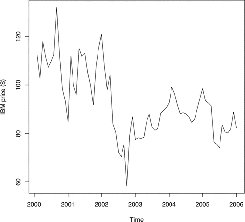
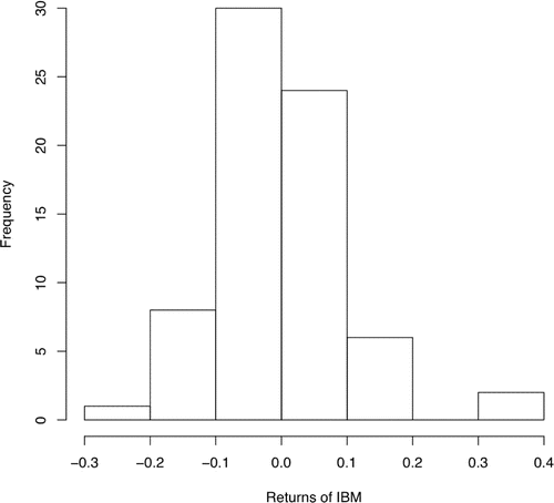
In some finance textbooks, instead of the denominator being n−1 (expressions (2) and (3)), they use n which is based on the maximum likelihood estimates (Rice, 1995). The corresponding histogram of the returns of IBM from January 2000 to December 2005 is shown in Figure 2. Investing in the stock market always bears some risk, large or small, depending on the variance of the returns of the stock. A stock that has large variance may make you rich but may also make you poor!

Figure 2: Returns of IBM, January 2000 - December 2005.

Therefore, risk is synonymous with variance and if investors are risk averse they want to minimize risk. Suppose now that the investor has two stocks and wants to make an investment. There are many possibilities of course. One of them is to invest all his available funds in the first stock and nothing in the second, or vice versa, another possibility is to invest 50% of his funds in the first stock and the other 50% in the second stock (equal allocation), etc. Which investment should he choose? We will answer this below.

3. Minimizing the risk of the portfolio

Let R_A and R_B be the returns of stocks A and B respectively, and let x_A, x_B be the proportions of the available funds invested in each if the stocks. Then the resulting portfolio is x_AR_A + x_BR_B. A risk averse investor would like to minimize his or her risk; therefore, he or she wants to minimize the variance of the portfolio:

which is subject to the budget constrained x_A + x_B = 1. If we incorporate the constraint in the variance of the portfolio we have the following unconstrained minimization (Chvatal, 1983):

(4)

The unknowns are x_A and x_B. By differentiating with respect to x_A, setting it equal to zero, and solving for x_A we get the following solution for x_A:

(5)

and therefore:

(6)

Note that the above expressions make sense in the following way. If var(R_A) > var(R_B), which means A is riskier than B, we would want to invest more in stock B than in A in order to minimize the risk of the portfolio. The problem of portfolio theory is not very old. Harry Markowitz is considered the pioneer in the area where in the early 1950s he published his work (Markowitz, 1952) to receive the Nobel prize much later in 1990. One question that immediately arises here is that the values of the variances and covariances are only estimates and are based on historical data. How well history predicts the future in stock market is another story, but it is better than having nothing. In the next sections we will present the results when two and three stocks are involved using real stock market data.

4. Portfolio management with two stocks

Monthly stock market data were obtained for the stocks IBM, EXXON-MOBIL, and BOEING (they are traded in the New York Stock Exchange (NYSE)), for the period January 2000 until December 2005. The data were obtained from the Wharton Research Data Services website (Center for Research in Security Prices, CRSP) at http://wrds.wharton.upenn.edu.

Table 1: Descriptive statistics of the returns of IBM, Exxon-Mobil, Boeing.

	Mean	Min	Q1	Median	Q3	Max
IBM	0.000307	−0.226453	−0.051552	−0.008992	0.046255	0.353799
EXXON-MOBIL	−0.001167	−0.521923	−0.017227	0.000701	0.033749	0.226938
BOEING	0.010791	−0.345703	−0.043080	0.018433	0.073570	0.174825

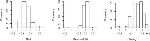
We first obtained the closing monthly prices which are then converted into monthly returns using (1). Figure 3 shows the fluctuations of the closing prices of the three stocks over time and Figure 4 shows the histograms of the returns of the three stocks. The mean returns of the three stocks are presented in Table 1, and the variance-covariance matrix of the returns of the three stocks is presented in Table 2. In this first example, we will use the IBM and BOEING stocks to find the most efficient portfolios.

Figure 3: Closing prices of IBM, Exxon-Mobil, Boeing, January 2000 - December 2005.

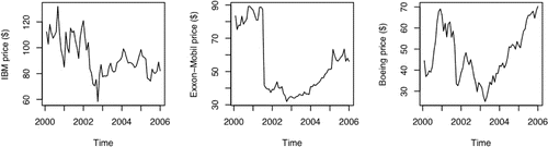
Figure 4: Returns of IBM, Exxon-Mobil, Boeing, January 2000 - December 2005.

The value of x_A using (5) is:

and therefore x_B = 1-x_A = 1 − 0.455 = 0.545. Therefore if the investor invests 45.5% of the available funds into IBM and the remaining 54.5% into BOEING, the variance of the portfolio will be minimized and equal to:

The corresponding expected return of this porfolio will be

We already see the benefit of diversification. The combination of 45.5% IBM and 54.5% BOEING gives less risk than the individual stocks.

Table 2: Variace-covariance matrix of IBM, Exxon-Mobil, Boeing.

	IBM	EXXON-MOBIL	BOEING
IBM	0.009930
EXXON-MOBIL	0.001799	0.006744
BOEING	0.000030	0.001781	0.008282

Table 3: Expected return and standard deviation on the portfolio for values x_A, x_B.

xA	xB	E(Rp)	σp
1.0	0.0	0.000307	0.099649
0.9	0.1	0.001355	0.090175
0.8	0.2	0.002404	0.081830
0.7	0.3	0.003452	0.074991
0.6	0.4	0.004501	0.070102
0.5	0.5	0.005549	0.067587
0.4	0.6	0.006597	0.067711
0.3	0.7	0.007646	0.070459
0.2	0.8	0.008694	0.075547
0.1	0.9	0.009743	0.082542
0.0	1.0	0.010791	0.091005

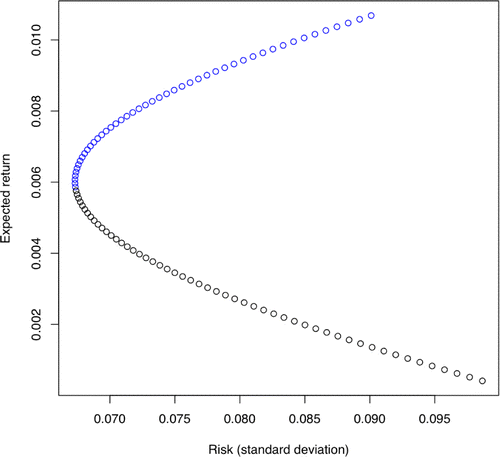
Of course not everyone would invest his or her funds in the above combination of the two stocks because some people can tolerate more risk than the minimum risk. Any other combination of the two stocks, (under the constraint x_A + x_B = 1), will give risk higher than the minimum risk that we have found. We can try many other combinations of x_A and x_B and compute the risk and expected return for each resulting portfolio. Some of these calculations are shown in Table 3. Now, let us plot the expected return against the risk (standard deviation) for each combination (portfolio). This graph is called the portfolio possibilities curve (Figure 5). We note here that the efficient portfolios are located on the top part of the graph between the minimum risk portfolio point and the maximum return portfolio point, which is called the efficient frontier (the blue portion of the graph). Efficient portfolios should provide higher expected return for the same level of risk or lower risk for the same level of expected return. Based on the investor's risk tolerance, his or her portfolio will be located on this efficient frontier (Elton et al, 2003).

Figure 5: Portfolio possibilities curve for two stocks.

5. Portfolio management with three stocks

When more than two stocks are involved in order to find the minimum risk portfolio we need to minimize:

(7)

or

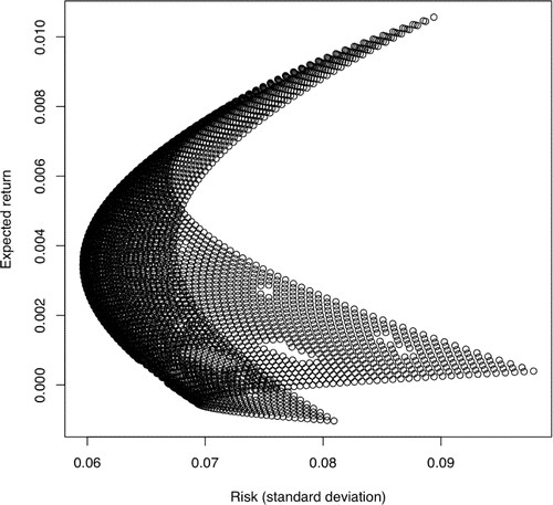
which is subject to the constraint x_A + x_B + x_C = 1, where x_A, x_B, x_C are the proportions of the available funds invested in the three stocks A, B, C respectively. The problem becomes more complicated as the number of stocks increases. This can be solved through quadratic programming (Bazarra, Shetty, 1979), but is easier to solve using some smart techniques that have been developed (Elton et al, 1977), which will not be discussed in this paper. Here we will only present the graph of the expected return against risk of the portfolio for various values of x_A, x_B, x_C (Figure 6). The three stocks used are IBM, EXXON-MOBIL, and BOEING. Each point on the graph represents a different portfolio. Again, we see that the efficient frontier is the part of the graph that connects the minimum risk portfolio to the maximum return portfolio (concave shape). The solution to the problem is to trace out this efficient frontier because that is where the investor finds his or her efficient portfolios.

Figure 6: Portfolio possibilities curve for three stocks.

6. Why does diversification work?

This section is intended for instructors and students who want to explore the topic with more rigor. We will explain here very briefly (Elton et al, 2003) why investing in more than one security reduces the risk. Suppose in the portfolio there are n securities. Then, the variance of the return on the portfolio (risk) is:

Let us consider equal allocation into the n securities. This means that of our wealth will be invested in each security. So, and the above expression becomes:

We can factor out from the first summation and from the second summation and since there are all together n(n-1) covariances we have:

We see that when n is large the risk of the portfolio is approximately equal the average covariance. The individual risk of securities can be diversified away. Even though equal allocation is not the optimum solution, it can explain the reduction of the portfolio risk when holding many securities. Moreover, it also explains why diversification reduces the risk when investing in securities that are uncorrelated or in securities for which the average covariance is small.

7. Conclusion

We have presented a brief theory on portfolio risk management and why it works. The two examples (with two and three stocks) using real market data can be used in class to enhance the teaching of covariance, correlation, and optimization. For this paper, all the analysis was done using R. However, it is also important to note here that the same analysis can be done using any other statistical software, as well as Matlab and Microsoft Excel. There are of course many other issues in portfolio theory that the interested reader may want to explore. For example, one may study some simple techniques for ranking stocks based on the excess return to beta or excess return to standard deviation, constructing portfolios using the single index model, the constant correlation model, the multi-index model, or the multi-group model (Elton et al, 1977). In addition, risky assets can be combined with risk-less securities (e.g. with a 90-day Treasury Bill). In this case, the risk of the portfolio will decrease. When I first started teaching this topic in my probability and statistics classes (I spent 1–2 lectures), I noticed that students showed a lot of interest in this area. The material was well received by the students who engaged in discussion of the subject. As a result of this, I proposed and taught once a year a new course “Statistical Models in Finance” that attracts many students from Mathematics, Engineering, Statistics, Biostatistics, as well as graduate students from Statistics, Economics, Computer Science, and Engineering. In finishing this paper we would like to mention the many applications of statistics to finance not only portfolio theory but also to areas such as options and futures (binomial theorem and the famous Black-Scholes model, (Hull, 2006). Some of these topics are advanced and require strong mathematical background but it is worthwhile exploring the teaching possibilities that these topics have to offer.

References

- Bazarra, M., Shetty, C. (1979). Nonlinear Programming, Theory and Algorithms. Wiley.
- Chvatal, V. (1983). Linear Programming. Freeman.
- Cox, D. R. (1998). Some remarks on statistical education. Journal of the Royal Statistical Society Series D-the Statistician, 47, 211–213.
- DeGroot, M., Schervish, M. (2002). Probability and Statistics. Addison Wesley, Third Edition.
- Dinov, I., Sanchez, J., and Christou, N. (2006). Pedagogical Utilization and Assessment of the Statistic Online Computational Resource in Introductory Probability and Statistics. Computers & Education in press (doi:10.1016/j.compedu.2006.06.003).
- Elton, E., Gruber, M., Brown, S., Goetzmann, W. (2003). Modern Portfolio Theory and Investment Analysis. Wiley, Sixth Edition.
- Elton, E., Gruber, M., Padberg, M. (1977). Simple Rules for Optimal Portfolio Selection: The Multi Group Case. The Journal of Financial and Quantitative Analysis, Vol. 12, No. 3, pp. 329–345.
- Hawkins, A. (1997). Discussion: Forward to basics! A personal view of developments in statistical education. International Statistical Review, 65, 280–287.
- Hull, J. (2006). Options, Futures And Other Derivatives. Prentice Hall, Sixth Edition.
- Markowitz, H. (1952). Portfolio Selectio. The Journal of Finance, Issue 1, pp. 77–91.
- Rice, J., (1995). Mathematical Statistics and Data Analysis. Duxbury, Second Edition.
- Stewart, J. (1999). Calculus. Brooks-Cole, Fourth Edition.
- Taplin, R. H. (2003). Teaching statistical consulting before statistical methodology. Australian & New Zealand Journal of Statistics, 45, 141–152.
- Teugels, J. L. (1997). Discussion: Forward to basics! A personal view of developments in statistical education. International Statistical Review, 65, 287–288.