Introduction to Multiple Regression: How Much Is Your Car Worth?

Abstract

Data collected from Kelly Blue Book for several hundred 2005 used General Motors (GM) cars allows students to develop a multivariate regression model to determine car values based on a variety of characteristics such as mileage, make, model, engine size, interior style, and cruise control. Students learn to look at residual plots to check for heteroskedasticity, normality, autocorrelation, and multicollinearity as well as explore techniques for variable selection and develop specially constructed variables.

• Multiple Regression
• Dummy Variables
• Heteroskedasticity
• Data Transformation
• Residuals

1. Introduction

This paper discusses the development of a multivariate regression model to predict the retail price of 2005 General Motor (GM) cars. Statistical textbooks typically offer many small data sets chosen to illustrate a variety of issues and techniques that a user of regression should know. Although small data sets can offer the advantage of sharp focus on particular issues, their narrow focus carries disadvantages as well. Working with a large, richly structured data set can give students a kind of experience not possible with a succession of smaller data sets. Accordingly, many courses use projects to ensure that students experience the challenge of model building and the opportunity to synthesize the elements of regression learned one at a time from smaller data sets. However, students can often have difficulty adjusting from traditional homework to a true research project that requires transitioning from a research question to a statistical model, properly collecting and cleaning data, appropriate model building and assessment, as well as effectively communicating their results. The structure of this data set allows students to work through the entire process of model building and assessment, thus providing a guided practice run before tackling a large data set on their own. This bridges the gap between short, focused homework problems and the open-ended nature of a project.

This data set was created in order to provide a rich interdisciplinary example that serves as a guide through the complete process of a multiple regression analysis project. The price of cars is an example of general interest to students and does not require specialized knowledge. This context is common enough that it may also aid many students in their conceptual understanding of the substantive issues related to regression.

For this data set, a representative sample of over eight hundred 2005 GM cars were selected, then retail price was calculated from the tables provided in the 2005 Central Edition of the Kelly Blue Book (see Section 11). Students are provided with a data set containing the following variables:

• Price: suggested retail price of the used 2005 GM car in excellent condition. The condition of a car can greatly affect price. All cars in this data set were less than one year old when priced and considered to be in excellent condition.

• Mileage: number of miles the car has been driven

• Make: manufacturer of the car such as Saturn, Pontiac, and Chevrolet

• Model: specific models for each car manufacturer such as Ion, Vibe, Cavalier

• Trim (of car): specific type of car model such as SE Sedan 4D, Quad Coupe 2D

• Type: body type such as sedan, coupe, etc.

• Cylinder: number of cylinders in the engine

• Liter: a more specific measure of engine size

• Doors: number of doors

• Cruise: indicator variable representing whether the car has cruise control (1 = cruise)

• Sound: indicator variable representing whether the car has upgraded speakers (1 = upgraded)

• Leather: indicator variable representing whether the car has leather seats (1 = leather)

Students are first asked to use simple linear regression to explore the intuitive relationship between miles traveled and retail price. The R-Sq value of this relationship is 2%, but after a closer look at the residuals, a transformation, and appropriate variable selection, students are able to develop a very strong multiple regression model. In addition, students learn that there isn't always just one “best” model when conducting data analysis.

Students work through this data set in a step-by step guided lab in groups of 2 or 3 as part of a final project in an introductory statistics course. While some of the work is done outside of class, about two class sessions in a computer lab should be planned for students to work through the lab and ask questions. This course has a calculus requirement and currently is using Chance and Rossman's workshop-style text Investigating Statistical Concepts, Applications, and Methods. Students have been introduced to simple linear regression and inference for simple linear regression before being introduced to this data set. After students walk through this guided lab, they are asked to conduct a multivariate regression analysis and create a research poster on a different data set in a completely different context as their final project. This data set is also used as a lab module in a second statistics course. The only prerequisite for this second statistics course is an AP style introductory course.

2. The Need for Multiple Regression: Regress Price on Mileage

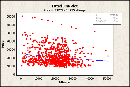
Before developing a complex multiple regression model with several variables, students start with a quick review of the simple linear regression model by asking a question: “Are cars with lower mileage worth more?” Clearly it seems reasonable to expect to see a relationship between mileage (number of miles the car has been driven) and retail value. Hence students try fitting a simple linear regression model relating price with mileage, and obtain the following results:

Equation 1:

The t-statistic for the slope coefficient (b₁): t = −4.09 (p-value < 0.001)

R-Sq: 2.0%

These results can lead to some nice review questions, such as:

1)	In general, what happens to price when there is one more mile on the car?
2)	Does the fact that b1 is small (−0.17) mean mileage is not very important? Students often misinterpret the magnitude of b1 as a measure of significance. Here students get a feeling of the importance of scale. For example, “How does the price change if two cars are identical except one has 60,000 more miles?” Students see that b1 = −0.17 can be meaningful since mileage has so much variability.
3)	Does mileage help you predict price? What does the p-value tell you?
4)	Does mileage help you predict price? What does the R-Sq value tell you?

Traditional textbook examples usually have data that fit very nicely, with high R-sq and low p-values. For this example, however, many students feel the simultaneously small p-value and small R-Sq value send contradictory messages about the model. The p-value for b₁ indicates that mileage is an important variable, but the R-Sq value shows that the model does not account for much of the variation in retail prices. This also illustrates that it is always better to take a few minutes to visualize any data set instead of solely focusing on a p-value. The scatterplot in Figure 1 and R-Sq value suggest that including other explanatory variables in the regression model might help to better explain the variation in retail price.

Figure 1: Scatterplot of retail price and mileage.

This plot also provides a nice starting point for discussing the importance of checking for outliers and influential observations. The scatterplot reveals a set of data points with retail prices higher then $52,000 that don't seem to fall in the general cluster of data. Students identify these cars as all being Cadillac XLR-V8 (a hardtop convertible), clearly a car that tends to be more expensive than average. This is used as an example to show students that potential outliers should not automatically be eliminated from the data set.

Also notice that the price of the 10 Cadillac XLR-V8 vehicles has a strong linear relationship with mileage (R-Sq = .99). The difference in R-Sq (99% here versus only 2% for the entire data) illustrates an important phenomenon: the strength of the relationship can be highly dependent on the set of cases, and whether they are homogeneous or heterogeneous, with respect to the predictor, and with respect to the other variables that are not part of the model.

3. Variable Selection Techniques

If the goal of developing a regression model is to describe or predict the retail price of a car, one of the primary issues is determining which variables to include in the model (and which to leave out). Clearly, all potential explanatory variables could be included, but that often results in a cumbersome model that is difficult to understand. On the other hand, a model that includes only one or two explanatory variables may provide substantially different predictions than the complex model. This tension between finding a simple model and finding a model that best explains the response is what makes it difficult to find a “best” model. This data set provides opportunities to discuss variable selection techniques to find models that provide a high R-Sq value while limiting the number of variables, such as Mallows' Cp, the Akaike information criterion, or stepwise regression.

For example, the best subsets technique in Minitab provides the output shown in Figure 2. At this point in the lab dummy variables have not yet been discussed, thus the output is restricted to the quantitative and binary explanatory variables. This output included the following from Minitab:

Figure 2: Output from the best subsets technique in Minitab. Only the best two models for each number of variables (Vars.) are displayed.

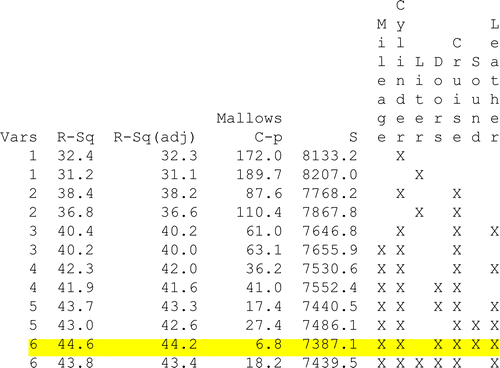
The following definitions are taken directly from Minitab help:

• “Vars” lists the number of predictors in each model.

• R-Sq describes the proportion of variation in the response data explained by the predictors in the model.

• Adj. R-Sq is a modified version of R that has been adjusted for the number of predictors in the model.- similar to choosing model with smallest MSE

• Mallows Cp is a measure of the error in the best subset model, relative to the error incorporating all variables. Adequate models are those for which Cp is roughly equal to the number of parameters in the model (including the constant), and/or Cp is at a minimum.

• s is the standard deviation of the error term in the model

• Predictor columns, one for each predictor, are the last columns in the table. These columns indicate whether the corresponding predictor is included in the model. Predictors included in the model are marked with an X.

A good model should have high R and adjusted R, small s, and Cp close to the number of predictors contained in the model.

Mallows Cp is used to compare models with a similar number of predictors (Vars). When using Mallows Cp to select a model with a specific number of predictors, a model should be chosen where Mallows Cp is as close as possible to the number of predictors (including the constant) in the model. Several texts [e.g. Draper and Smith (1981), Neter et. al., (1985), and Ramsey and Schefer (2002)] and papers [e.g. Mallows, (1973) and Hocking, (1976)] discuss these techniques in more detail. In Figure 2, if a student wanted to select a model with six explanatory variables, the highlighted row has the best Cp and R-Sq values. This highlighted row corresponds to using Mileage, Cylinder, Doors, Cruise, Sound, and Leather as explanatory variables. The suggested best subsets regression equation is:

Equation 2: Predictor Coef SE Coef T P Constant 7323 1771 4.14 0.000 Mileage −0.17052 0.03186 −5.35 0.000 Cyl 3200.1 203.0 15.77 0.000 Doors −1463.4 308.3 −4.75 0.000 Cruise Control 6205.5 651.5 9.53 0.000 Premiun Sound −2024.4 570.7 −3.55 0.000 Leather 3327.1 597.1 5.57 0.000 S = 7387.11 R-Sq = 44.6% R-Sq(adj) = 44.2%

This model has a much better R-Sq value than Equation 1 and it appears that all the explanatory variables in this model are important. However, as the next sections show, simply using a variable selection technique does not guarantee a “best” regression model.

4. Goals of Multiple Regression

Often, examples in statistics courses describe iterative techniques to find the model that best describes relationships or best predicts a response variable. This data set can also demonstrate how multivariate regression models can be used to confirm theories. The most common goals of multiple regression are to:

1)	Describe: Develop a model to describe the relationship between the explanatory variables and the response variable.
2)	Predict: Use a set of sample data to make predictions. A regression model can be used to predict response values from explanatory variables within the range of our sample data.
3)	Confirm: Theories are often developed about individual variables, such as confirming which variables, or combination of variables, need to be included in the model. Regression can then be used to determine if the contribution of each explanatory variable in a model captures much of the variability in the response variable.

The techniques used may depend upon the objectives of the analysis. The focus when using iterative variable selection techniques is not the significance of each explanatory variable, but how well the overall model fits. However, if the goal is to confirm a theory, other methods should be used.

This data set provides an example of how an economist might use multiple regression analysis to formulate a focused hypothesis based on theory. This includes determining if the association between specific explanatory variables and the response could just be due to chance. For example, an economist may choose to test if mileage should be used to predict retail price or if cars with more cylinders cost more. Confirming a theory is similar to hypothesis testing. Iterative variable selection techniques test each variable, or combination of variables, several times and thus the p-values are not reliable. The stated significance level for a t-statistic is only valid if the data are used for a single test. If multiple tests are conducted to find the best equation, the p-value reported by software for each test for an individual component is invalid because numerous non-independent tests were done.

Theories are also developed about the type of relationship that exists, such as “cars with lower mileage are worth more”. In these situations, economists are testing whether the sign of the regression coefficient is consistent with their hypothesis. More specific theories, such as “retail price decreases linearly with mileage” can also be tested. In these situations, a hypothesis test is needed to determine if the regression coefficients are significant, thus the variables selected to be used in the regression equation should be based on theory. Often variables that would be considered as practically important in a model are inappropriately eliminated in these automated iterative techniques. While highly correlated predictors tend not to be included in a suggested model, multicollinearity is not specifically addressed in Mallows' Cp, Akaike's information criterion, or stepwise regression. As discussed in the multicollinearity section, variables excluded from the suggested best subsets model, such as Liter, may still be highly correlated with the response variable. The out-of-print text by Mosteller, Fieinberg, and Rourke (1983) provides a nice discussion of the aims of fitting regression models.

5. Exploring Patterns

Before Equation 2 is considered acceptable, students are encouraged to check the model assumptions. While the Minitab output indicates each of these six predictors is significant, the residual plots shown in Figure 3 reveal that there clearly are still violations of the model assumptions. Thus the hypothesis tests should not be taken at face value.

Normally Distributed Error Terms: The histogram and normal probability plot of residuals show that the error terms are not normally distributed: in particular, there is a long upper tail, which corresponds to the outlying points visible in the regression plot in Figure 1.

Heteroskedasticity (non-constant variance): The Residual vs. Fitted values plot shows some clustering and the variability of the residuals depends on the fitted value. There is more variability around the regression line when prices are higher. Consider a vertical slice of Figure 1, for example the rectangle formed to include all Y values when mileage ranges from 15000 to 16000 miles. Looking at the distribution of y-values within vertical slices does show a high degree of skewness. Often such skewed conditional distributions for Y|X suggest transforming to roots, logs, or reciprocals. Students can try suggested transformations of the data and then create similar residual plots for the transformed data. In this data set, the transformed variable, TPrice = log(price), is useful in addressing the violations of the model assumptions.

Figure 3: Residual plots for Equation 2.

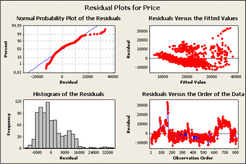
Residuals versus order in the data: Figure 3 addresses another interesting aspect of this data set in the strong pattern in the ordered residuals even though there is no time variable (all data is based on 2005 GM cars). While sequence plots only make sense in model checking when there is a meaningful order to the data, the residual versus order plots in Figures 3 and 4 have been very helpful in getting students to perceive the need for including additional explanatory variables in the regression model. The residual versus order plot shown in Figure 4 helps emphasize the pattern arising due to the Make and Model of the cars being listed in alphabetical order. Cars with the same Make and Model tend to have similar retail prices. Even though indicator variables have not yet been discussed, students understand that including Make as an explanatory variable could greatly reduce the residual values.

Figure 4: A residual versus order plot using Equation 1: Price = 24723 — 0.17 Mileage.

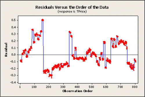
At this time, it should be clear that simply plugging data into a software package and using an iterative variable selection technique will not reliably create a “best” model. The following sections discuss techniques to address the model violations in order to create a better regression model.

6. Specially Constructed Explanatory Variables

The clusters in Figure 4 are easily identified from the listing of the data. The Make of these 2005 cars (Buick, Cadillac, Chevrolet, Pontiac, SAAB, and Saturn) are related to the price, and students see a need to incorporate categorical variables into their models.

To incorporate categorical variables into a regression model, students have the opportunity to create dummy variables, also called indicator variables. Creating dummy variables is a process of mapping one column of categorical data into several columns of 0 and 1 data. In this data set, dummy variables can be created for Make, Model, Trim and Type. Using the variable Make as an example, the six possible values (Buick, Cadillac, Chevrolet, Pontiac, SAAB, and Saturn) can be recoded using six dummy variables: one for each of the six Makes of car. For example, the dummy variable for Buick will have the value 1 for a car that is a Buick and 0 for any car that is not a Buick.

Recall that to include Make in its entirety into the model, we do not include all six dummy variables; five suffice. There is complete redundancy in the sixth dummy variable. In the following regression models, Saturn was arbitrarily left out of the model. The slope coefficient for a dummy variable is an estimate of the average amount (of the response variable) by which a “1” for that dummy variable will exceed the baseline value, which in this case is Saturn.

7. Multicollinearity

Many students may have already noticed that powerful sports cars have higher prices. In this data set there are two measures of engine size, the number of cylinders (Cylinder) and the displacement volume (Liter). There is a strong relationship between these two variables. Notice that Equation 2 included Cylinder but did not include Liter. Students may have assumed that Liter simply was not useful in predicting price. The following exercise is beneficial in helping students understand the impacts of highly correlated explanatory variables.

Three regression models are developed with this data set to predict retail price: (1) Mileage and Liter, (2) Mileage and Cylinder, and (3) Mileage, Liter and Cylinder. The R-Sq values for all three models are similar; however, Liter and Cylinder are both measures of engine size. The R-Sq values and the t-tests for the regression coefficients show that Liter is significant in predicting Retail Price in Model 1. Similarly Cylinder is significant in Model 2. However, Model 3 only shows Liter as significant. Students have the opportunity to see that a useful predictor of the response variable can sometimes fail to register as statistically significant. Students learn the importance of identifying the presence of multicollinearity and to recognize that the coefficients are unreliable when it exists.

Students also learn that there is no “best” regression model. Often determining whether certain variables are included in a multivariate regression model depends on the goals of the study. If the coefficients are not being interpreted, highly correlated explanatory variables that both contribute to the model, such as Liter and Cylinder, could both be kept in the model. However, one of these redundant variables should be eliminated from the model if the goal is to confirm whether an explanatory variable is associated with a response (i.e. test a hypothesis). It is important to note that researchers using an iterative regression technique could have incorrectly concluded that Cylinder is not important in predicting retail price. In the following analysis, Cylinder will be eliminated from the data, since Cylinder and Liter are both measures of engine size, but Liter is more precise.

Iterative techniques can be used to suggest the following model when using dummy variables for Make, TPrice = log(price), and eliminating Cylinder.

Equation 3: Predictor Coef SE Coef T P Constant 3.97991 0.00928 429.05 0.000 Mileage −0.00000348 0.00000022 −15.61 0.000 Liter 0.099725 0.002000 49.87 0.000 Buick 0.039969 0.009200 4.34 0.000 Cadillac 0.249303 0.009726 25.63 0.000 Chev −0.009372 0.007336 −1.28 0.202 Pontiac 0.013613 0.008116 1.68 0.094 SAAB 0.345305 0.008236 41.93 0.000 S = 0.0515753 R-Sq = 91.7% R-Sq(adj) = 91.6%

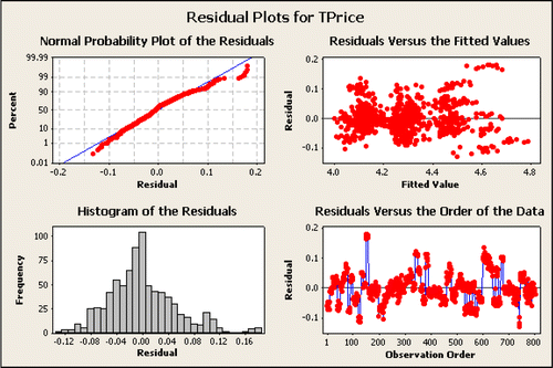
This shows a clear improvement over Equation 1 and 2. The R-Sq is much better and the patterns in the corresponding residual plots shown in Figure 5 are much attenuated.

Figure 5: Minitab plots of the residuals for the Equation 3: TPrice = 3.98 – 0.000003 Mileage + 0.0997 Liter + 0.0400 Buick + 0.249 Cadillac – 0.00937 Chev + 0.0136 Pontiac + 0.345 SAAB. The histogram and normal probability plot show that the error terms are not normally distributed. The plot of Residuals vs. Fitted values looks better but some clustering is still visible. The Residuals vs. Order plot also shows some systematic patterns, but they are much less pronounced than before.

Students are also encouraged to try other models by including additional variables in the model. Including the other variables in the data set will improve the R-Sq value somewhat. In addition, including the other variables will create a model that fits the regression assumptions. Equation 4 using Make, Trim, Mileage, Liter, Doors, Cruise, Sound, and Leather would appear to be a reasonable model. Minitab output for this suggested model is given below. Note that Minitab and SPSS (though not shown here) will automatically eliminate one of the Trim dummy variables, Coup, because it was highly correlated with other explanatory variables. The corresponding regression equation is:

Equation 4: Predictor Coef SE Coef T P Constant 3.91811 0.01231 318.26 0.000 Mileage −0.00000358 0.00000017 −21.02 0.000 Liter 0.095762 0.001721 55.64 0.000 Doors 0.033527 0.003518 9.53 0.000 Cruise 0.007517 0.004009 1.88 0.061 Sound 0.005223 0.003170 1.65 0.100 Leather 0.006260 0.003397 1.84 0.066 Buick 0.041653 0.007441 5.60 0.000 Cadillac 0.233034 0.007944 29.33 0.000 Chev −0.013315 0.005950 −2.24 0.026 Pontiac −0.000421 0.006519 −0.06 0.949 SAAB 0.281098 0.007481 37.58 0.000 Conv 0.137819 0.007306 18.86 0.000 Hatchback −0.088989 0.008164 −10.90 0.000 Sedan −0.071149 0.006019 −11.82 0.000 S = 0.0393651 R-Sq = 95.2% R-Sq(adj) = 95.1%

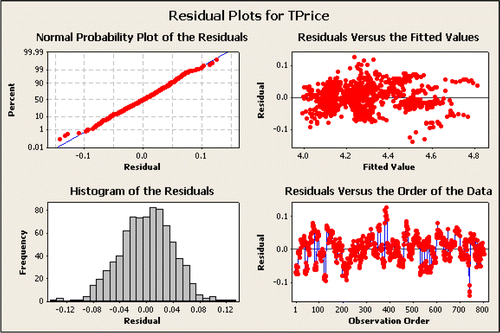
The R-Sq and R-Sq(adj) are slightly higher in Equation 4 and Figure 6 below shows that the model assumptions appear to be satisfied. If iterative techniques were not used and the model assumptions hold, it would be reasonable to use hypothesis testing to conduct inference on each of the regression coefficients.

Figure 6: Residual plots for Equation 4: a multivariate regression model to predict TPrice with Make, Trim, Mileage, Liter, Doors, Cruise, Sound, and Leather as explanatory variables. The residuals appear to be homoskedastic and more closely follow a normal distribution. The Kolmogorov-Smirnov (K-S) test for normality resulted in a p-value = 0.13. The residual vs. order plot has much less clustering. Students may want to consider including Model as a predictor, but the corresponding set of dummy variables is very large, and adding them to the model doesn't improve R-Sq.

8. Interaction and Terms for Curvature

Students also have the opportunity to create quadratic and interaction terms in their regression model, such as Mileage*Liter, Liter*Liter, Mileage*Cylinder, and Cylinder*Cylinder.

None of the quadratic or interaction terms noticeably improve the model described above. However, the benefits of a quadratic model can be demonstrated by comparing Price = bo + b1Cylinder and Price = bo + b1Cylinder + b2Cylinder^2.

The line of outlying points identified in Figure 1 can provide an interesting demonstration of interaction terms. The fitted slope to predict price from mileage is -.48 for the 10 Cadillac LXR-V8s, much steeper than the -.17 found in Equation 1 using the data set as a whole. This shows that depreciation for these high-end cars is almost 50 cents a mile, as opposed to 17 cents a mile when using the entire data set. Notice that Equation 4 shows that Cadillac, Liter and convertible are all in the final model. Each of these variables tends to represent high-end cars. This may motivate students to attempt to develop additional interaction terms that may create an even better model.

9. Conclusion

This data set provides a real economics example that is of interest to students and at the same time does not require deep knowledge of economic theory. We have used this data set as a guided introduction to multivariate regression that encourages students to try various models and demonstrate the importance of checking model assumptions.

This guided lab activity encourages students to think like a statistician when working with advanced regression techniques. While this data set and lab were originally created to be used in a second statistics course, we have also used this lab as part of a final project for talented students in introductory statistics classes. This data set and lab are particularly helpful for students planning on conducting research in economics.

This is one of several lab modules we are developing to emphasize the process of data analysis relevant for science and social science students. This helps students and future researchers in many fields to understand the conditions under which studies should be conducted and gives them the knowledge to discern when appropriate techniques should be used.

10. Availability

The data set, student lab handout with Minitab instructions, and instructors' notes for this activity are available at http://web.grinnell.edu/individuals/kuipers/stat2labs/topics.html.

11. Kelly Blue Book Data

Kelly Blue Book has been a resource for accurate vehicle pricing for over 80 years. The website, www.kbb.com, is also a free on-line resource to calculate estimated retail price. According to Kelly Blue Book representatives, there is no single regression model or data base that is used to calculate their estimates. They have a very complex series of databases and models that are merged and weighted to determine price for various geographical regions.

12. Acknowledgements

Partial support for this work was provided by the Course, Curriculum, and Laboratory Improvement program at the National Science Foundation under DUE 0510392. I would like to thank Tom Moore and Linda Collins for their contribution to this project. I also thank the editor and two anonymous reviewers for their many helpful suggestions.

Appendix A

Data Description

NAME: 2005 Car Data

TYPE: Multiple Regression

SIZE: 810 observations, 12 variables

DESCRIPTIVE ABSTRACT:

Data collected from Kelly Blue Book for several hundred 2005 used GM cars allows students to develop a multivariate regression model to determine their car value based on a variety of characteristics such as mileage, make, model, engine size, interior style, and cruise control. Students learn to look at residual plots and check for heteroskedasticity, autocorrelation, and multicollinearity.

SOURCES:

For this data set, a representative sample of over eight hundred, 2005 GM cars were selected, then an algorithm was developed following the 2005 Central Edition of the Kelly Blue Book to estimate retail price.

VARIABLE DESCRIPTIONS:

Price: suggested retail price of the used 2005 GM car in excellent condition. The condition of a car can greatly affect price. All cars in this data set were less than one year old when priced and considered to be in excellent condition.

Mileage: number of miles the car has been driven

Make: manufacturer of the car such as Saturn, Pontiac, and Chevrolet

Model: specific models for each car manufacturer such as Ion, Vibe, Cavalier

Trim (of car): specific type of car model such as SE Sedan 4D, Quad Coupe 2D

Type: body type such as sedan, coupe, etc.

Cylinder: number of cylinders in the engine Liter: a more specific measure of engine size Doors: number of doors Cruise: indicator variable representing whether the car has cruise control (1 = cruise)

Sound: indicator variable representing whether the car has upgraded speakers (1 = upgraded)

Leather: indicator variable representing whether the car has leather seats (1 = leather)

Link to Data Set: http://ww2.amstat.org/publications/jse/v16n3/kuiper.xls

References

- Chance, B., and Rossman, A., (2006), “Investigating Statistical Concepts, Applications, and Methods”, Duxbury.
- CUPM Curriculum Guide (2004), A report by the Committee on the Undergraduate Program in Mathematics of The Mathematical Association of America. http://www.maa.org/cupm/cupm2004.pdf
- Draper, N.R. and Smith, H., (1981), “Applied Regression Analysis”, Wiley.
- Hocking, R.R. (1976), “The Analysis and Selection of Variables in Linear Regression”, Biometrics, 32, 1–50.
- Kelley Blue Book, (2005), Central Edition, www.kbb.com
- Mallows, C.L. (1973), “Some Comments on Cp”, Technometrics, 15, 661–675.
- Moore, T., Peck, R., and Rossman, A. (2000), “Calculus Reform and the First Two Years (CRAFTY).” http://www.maa.org/cupm/crafty/cf_project.html
- Mosteller, F., Fienberg, S., and Rourke, R. (1983), Beginning Statistics with Data Analysis, pp 302–307, Addison Wesley
- Neter, J., Wasserman, W., and Kutner, M. (1985), Applied Linear Statistical Models, Homewood, Illinois: Irwin.
- Ramsey, F.L. and Schafer, D.W., (2002), The Statistical Sleuth, Duxbury.
- Undergraduate Statistics Education Initiative (USEI), in 1999 a committee funded by ASA met to “Promote Undergraduate Statistics to Improve the Workforce of the Future”. This initiative has led to multiple workshops and symposiums. http://ww2.amstat.org/education/index.cfm?fuseaction=usei