Long-Term and Seasonal Trends of Wastewater Chemicals in Lake Mead: An Introduction to Time Series Decomposition

ABSTRACT

A recent paper published time series of concentrations of chemicals in drinking water collected from the bottom of Lake Mead, a major American water supply reservoir. Data were compared to water level using only linear regression. This creates an opportunity for students to analyze these data further. This article presents a structured introduction to time series decomposition that compares long-term and seasonal components of a time series of a single chemical (meprobamate) with those of two supporting datasets (reservoir volume and specific conductance). For the chemical data, this must be preceded by estimation of missing datum points. Results show that linear regression analyses of time series data obscure meaningful detail and that specific conductance is the important predictor of seasonal chemical variations. To learn this, students must execute a linear regression, estimate missing data using local regression, decompose time series, and compare time series using cross-correlation. Complete R code for these exercises appears in the supplementary information. This article uses real data and requires that students make and justify key decisions about the analysis. It can be a guided or an individual project. It is scalable to instructor needs and student interests in ways that are identified clearly in this article.

KEYWORDS:

• Cross-correlation
• Environmental science
• Local regression
• Missing values
• Water quality
• Wastewater contaminant

1. Introduction

During the first decade of the 21st century, many water researchers studied the occurrence and treatment of pharmaceuticals, personal care products, and other organic chemicals in natural waters, wastewater, and drinking water (e.g., Sedlak 2014). These chemicals captured widespread attention because of their potential to disrupt human endocrine function, because they arouse disgust in water consumers, and because analytical chemistry technologies advanced so that these chemicals could be measured reliably at low concentrations (e.g., Colborn et al. 1997; Sedlak 2014). Many peer-reviewed papers have reported the occurrence of such chemicals. A recent study by Benotti et al. (2010) went further, suggesting a response of chemical concentrations in a reservoir to hydrologic change. These authors studied Lake Mead, the large reservoir in Arizona and Nevada, USA that is the main source of water for Southern Nevada. They found that, as the water level of Lake Mead declined during the years 2003–2007, inclusive, the concentration of a group of pharmaceuticals and other endocrine-disrupting chemicals (e.g., the herbicide atrazine) steadily increased. This led the authors to suggest that less water in Lake Mead implied less dilution of chemicals discharged to it and that this was evidence of climate change altering water quality, since the decreasing water level of Lake Mead can be partially attributed to climate change (Benotti et al. 2010).

Benotti et al. (2010) reached their conclusions regarding the opposite five-year trends of chemical concentrations and water level by conducting two separate linear regressions on nonlinear time series data. From an environmental chemistry and water management standpoint, these authors contributed valuable data to the literature and offered a reasonable interpretation of those data. However, their limited statistical analyses offer students a valuable opportunity to explore additional richness in a real, published, analytically costly, and practically relevant dataset. Structured investigation of this and related datasets provides a rigorous introduction to time series decomposition, which is described fully by Yafee and McGee (2000), Hyndman and Athanasopoulos (2015), and references therein. Doing so also requires an introduction to local regression and cross-correlation as well as critical thinking by students regarding statistical decision making. These techniques, their coding in R, and the presentation of figures that they generate are the focus of this article.

The author uses this exercise at the end of the time series unit of his Data Science B: Time Series and Multivariate Statistics course. Students come to this course having had either Statistics 1: The Practice of Statistics, AP Statistics in high school, or a strong quantitative background. The first major unit of Data Science B reviews prerequisite content in an applied context. It covers hypothesis testing, comparisons of related datasets, and linear regression. It also introduces students to writing scripts in R. Students in the course are usually either upper-year undergraduates who expect to generate significant data in their undergraduate theses or students focusing on applied math. The author's institution does not have majors, but nonmath students in this course tend to focus on ecology, health sciences, environmental science, or data science.

2. The Datasets and the Story

2.1. Background

The Colorado River flows more than 2300 km from the Rocky Mountains to the Gulf of California. The majority of its water comes from mountain snowmelt near its headwaters. Much of its watershed is arid. Major infrastructure projects allow diversion of water from the river to agricultural and municipal users. This consumptive use of water is highly regulated; in the downstream portion of the river, California, Arizona, and Nevada are allocated fixed volumes of water each year, each of which is used in its entirety (MacDonnell 2009). More water has been promised to users than flows down the Colorado River in an average year, and so the water storage of reservoirs on the river has decreased in most years of the 21st century (Barnett and Pierce 2008). This unsustainable situation is exacerbated by an ongoing, long-term decrease in annual flow volumes of the Colorado River, a phenomenon that may be caused by climate change (Webb et al. 2004; Barnett and Pierce 2008; USBR 2011a).

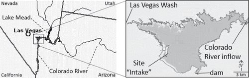
Nevada draws all its Colorado River water from a location deep in Lake Mead, the large reservoir formed by the iconic Hoover Dam (Figure 1), and distributes it to municipal and industrial users in Las Vegas and surrounding cities (USBR 2011a). The Las Vegas Valley also discharges its treated wastewater to Las Vegas Wash, a small river that flows directly to the surface of Lake Mead. This accounts for less than 2% of the inflows to Lake Mead; about 97% of inflows come from the Colorado River. Therefore, a small fraction of the water taken by Southern Nevada for municipal supply is highly diluted former wastewater. Because of this, the Southern Nevada Water Authority (SNWA), which coordinates seven utilities in southern Nevada, has developed extensive expertise in the treatment of water and wastewater.

Figure 1. Study location. Left panel: Southern Nevada and surrounding states; thick lines are state borders and thin lines are the Colorado River and tributaries of Lake Mead. Box indicates area shown in right panel. Right panel: Boulder Basin, the downstream portion of Lake Mead, which receives water from the upstream portion of Lake Mead and the Colorado River though the region marked “Colorado River inflow.” The river channel is on the east side of Boulder Basin. Las Vegas Wash enters Boulder Basin from the west. The intakes that supply water to Southern Nevada are located on the west side of Boulder Basin at the “Intake” site.

The SNWA has developed particular expertise in the measurement of wastewater-derived organic chemicals (WDOCs). These chemicals, which range from pharmaceuticals to personal care products (e.g., shampoo ingredients or insect repellent) to pesticides ingested with food, exist in treated wastewater because wastewater treatment facilities are not designed to remove them (e.g., Sedlak 2014). These chemicals have been measured in a variety of aquatic systems, such as groundwater (Barnes et al. 2008), untreated drinking water sources (Focazio et al. 2008), and finished drinking water (Benotti et al. 2009) across the United States. They have been studied extensively by specialists (e.g., Schwarzenbach et al. 2006; Kümmerer 2010, and references therein), but they are not regulated in surface waters or drinking water because health risks of chronic exposure to trace concentrations are unclear and acute health risks are low (Bruce et al. 2010). However, the SNWA practice of discharging treated wastewater to its drinking water source creates the possibility that concentrations of WDOCs in Lake Mead could increase over time despite considerable dilution because chemicals could be added to water more rapidly than they are degraded as water makes successive passes through the urban system.

Most studies of WDOCs in natural waters characterize their occurrence; few have explored connections between their concentrations and hydrological processes. In their paper, Benotti et al. (2010) studied 16 WDOCs in Lake Mead. They described repeated sampling at a specific deep-water location (the intake structure for the Southern Nevada water supply system), reported time series data of the summed concentration of the WDOCs analyzed, and evaluated trends over five years (2003–2007, inclusive) using linear regression. After controlling for other variables and possible explanations, they reported a long-term, significant, inverse relationship between water level and concentration of WDOCs in Lake Mead. They attribute decreasing water level to climate change and thus suggest a link between this phenomenon and water quality for a major city.

The chemical data collected by Benotti et al. (2010) were collected with sophisticated instrumentation that represented the state of the art of organic chemical analysis when their paper was published. However, analyzing their data only with linear regression and exploring only long-term trends does not exploit the full richness of their dataset. Time series analysis provides a useful tool to explore the data collected by Benotti et al. (2010) in much greater detail, and the data contain multiple complexities that enable a thorough introduction to time series for students. This exercise is designed to occur after an introduction to time series decomposition and local regression. It can be used as a thorough introduction to of time series analysis before students broach the complex topics of time series modeling and forecasting.

2.2. Data

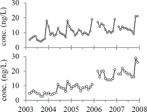
The primary dataset in this investigation consists of monthly concentrations of a suite of WDOCs collected by Benotti et al. (2010) from the SNWA drinking water intake at the bottom of Lake Mead (latitude: 36.06, longitude: −114.80). During the study period (March 2003 through December 2007), data were not collected in January 2006, February 2006, and January 2007. Benotti et al. (2010) took care to divide their chemical data into two sets because of an improvement in their analytical technique at the end of 2005 that allowed lower detection limits for most chemicals. Because they reported the sum of the 16 chemical concentrations that were measured above detection limits, this value increases after the change in analytical method. However, two chemicals, meprobamate (an antianxiety drug) and sulfamethoxazole (an antibiotic) are measured above detection limits in every sample using both methods. As a result, they are unaffected by the change in analytical method, and so their concentrations can be treated as single datasets with three missing datum points. To focus on data analysis rather than chemistry, this exercise analyzes only the meprobamate time series (subsequently referred to as the “chemical time series”). The sulfamethoxazole time series, which leads to similar yet not identical results, can also be studied. The data are contained in the data file “Lake_Mead_chemical_time_series.csv,” which is described by the documentation file “Lake_Mead_documentation_file.txt.” Meprobamate concentrations range from 4 to 21 ng/L with a median of 11 ng/L and an interquartile range (IQR) of 9–14 ng/L, and sulfamethoxazole concentrations range from 3 to 29 ng/L with a median of 10 ng/L and an IQR of 6–16 ng/L (Figure 2).

Figure 2. Observations of meprobamate (upper panel) and sulfamethoxazole (lower panel) concentrations measured in untreated water sampled from the drinking water intake in Lake Mead. Data from Benotti et al. (2010).

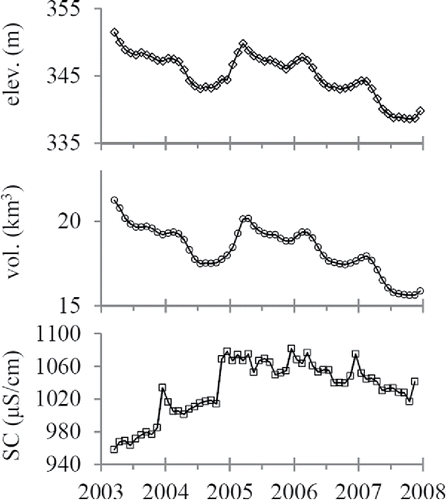
In addition to the chemical time series, three supporting datasets are included. Because Benotti et al. (2010) invoked dilution to explain the observed long-term relationship between chemical concentrations and water level, volume in Lake Mead is included to enable reconstruction of the claims of Benotti et al. (2010). Daily volumes of Lake Mead were calculated using water surface elevation and an empirical relationship between water elevation and volume derived from values reported by the USBR (2011b). Water elevation data were downloaded from the U.S. Bureau of Reclamation (USBR 2011c). At the end of this investigation, it is instructive for students to compare the seasonality of measured chemicals with the seasonality of specific conductance in Lake Mead, so these data are included as well. Specific conductance (SC) is a measurement of the ability of water to conduct electricity. It is closely linked to the concentration of dissolved ions. In environmental applications, most dissolved ions tend to react minimally, and so SC can be used to discriminate between different water masses. Previous studies have distinguished the treated wastewater entering Lake Mead from Las Vegas, which has high SC, from water entering Lake Mead from other sources, which has much lower SC (e.g., LaBounty and Burns 2005). The SC time series was downloaded for the SNWA monitoring site called “Intake” (latitude: 36.06, longitude: −114.80; SNWA 2011), which is located at the drinking water intakes (Figure 1). Daily data were converted to monthly data by taking arithmetic means of each month; monthly volume, SC, and elevation time series are found in the data file “Lake_Mead_volume_SC_elevation_time_series_monthly.csv.” Additionally, the daily time series is provided in a third data file called “Lake_Mead_volume_SC_time_series_daily.csv.” These two supporting files are described in the same documentation file as the chemical time series. During the study period, elevation decreased from a maximum of 352 m above sea level (asl) to a minimum of 340 m asl (Figure 3). Its median was 346 m asl. Correspondingly, volume decreased from 21.3 km³ to 15.6 km³ during the study period (Figure 3). Its median was 18.6 km³. The range of SC was 960–1080 μS/cm with a median of 1040 μS/cm and an IQR of 1010–1060 μS/cm (Figure 3).

Figure 3. Observations of Lake Mead elevation (upper panel), calculated Lake Mead volumes (middle panel), and observations of specific conductance (SC) at the Lake Mead drinking water intake (lower panel).

The data used in this exercise do not imply that the water supply of the people of Southern Nevada has ever been in danger of exceeding health standards or the best practices of the water supply industry. All water samples discussed here were measured before that water was treated for public consumption.

2.3. Research Tasks

This investigation focuses on five research tasks:

1. Reproduce the linear regressions of Benotti et al. (2010) and create an overlay graph of observations and their linear fit.

2. Estimate values for missing data in the chemical time series using local regression.

3. Decompose the chemical time series and assess goodness of fit.

4. Decompose the volume time series and compare its long-term trend to that of the chemical time series.

5. Decompose the SC time series. Compare the seasonal trend of the chemical data to the seasonal trends of the volume and SC time series using both overlay plots and cross-correlation.

Completing these tasks allows for the reproduction of the analysis conducted by the authors who collected the dataset, the demonstration of the shortcomings of fitting a linear model to seasonally variant time series data, and the use of time series decomposition to provide a more nuanced understanding of the data.

Helpful hint: The instructor might choose to have students act as reviewers for the Benotti et al. manuscript as a lead-in to this exercise. This can help students see why time series analyses are necessary, despite the ease of applying simpler techniques like linear regression inappropriately. It may also help them build emotional ownership over the results they produce in this exercise. When students have completed their reviews, a group discussion can be used to generate the list of tasks presented here with the instructor steering the group to create a complete list and perhaps improvising to allow students to explore any other analyses that they suggest.

Potential pitfall: In the experience of the author, students often require substantial amounts of time to review papers, especially when this is an entirely new activity to them. This can be because they seek to understand all parts of the content of the paper, which may be new to them. The instructor can facilitate a review assignment by explaining the Methods section carefully, providing a sheet defining strange terms (e.g., those about lakes or chemical names) and introducing all the variables that the students will encounter. Additionally, instructors might enforce a time limit of 2 to 3 hr to ensure that this prelude assignment does not exhaust students before they reach the assignment(s) described in this article, which can be more difficult.

3. The Analyses and Conclusions

The following subsections explain the statistical analyses that complete the research tasks listed above. Major statistical techniques used are as follows: linear regression, local regression, prediction (or imputation) of missing data, seasonal decomposition of time series by loess, and cross-correlation.

3.1. Research Task 1: Reproduce the Regressions and Conclusions of Benotti et al. (2010)

Regression of the chemical time series as a dependent variable on time as an independent variable is fairly straightforward with the lm command in R (all commands described here are for R version 3.1.2; R Core Team 2014). Plotting an overlay of the regression line (as represented by the set of fitted values that exists as an element of the object to which the lm command is assigned) on the original dataset shows the poor fit (Figure 4).

Figure 4. Meprobamate concentrations measured in Lake Mead by Benotti et al. (2010). The missing values in January 2006, February 2006, and January 2007 correspond to breaks in the black line.

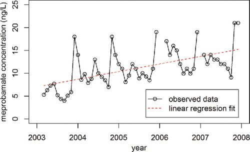
This task can be excluded for groups that have extensive experience in R, but, for other groups, it may be valuable because it introduces students to overlay plots in R (which are enabled by executing the command par(new = T) between plot commands). Additionally, this task, which is likely conceptually straightforward to students who are studying time series analysis, can be used to verify that students can use R for the basic tasks of reading in data, conducting a linear regression, and plotting actual and fitted values.

Helpful hint: This linear regression presents an opportunity to discuss with students that the viability of a linear regression, especially with regard to time, does not imply its appropriateness. There are two criticisms of the linear regression of chemical concentrations on time presented by Benotti et al. (2010). First, time series analysis is a much more appropriate approach because of the obvious temporal correlations and the seasonality and long-term trend in these data. Second, Benotti et al. (2010) invoke decreasing dilution as an explanation for the increasing concentration over time, since the water level and, implicitly, the volume of water in the reservoir was decreasing during this time. Therefore, a more appropriate linear regression analysis would regress chemical concentrations on Lake Mead volume (or elevation), since this is the relationship at the core of their interpretation.

Potential pitfall: If students are not comfortable writing an R script to read in data, execute a linear regression, and plot data, then this will be a very difficult assignment. For inexperienced students, the instructor may choose to divide this assignment into smaller assignments with individual deadlines so that students are forced to finish tasks and get feedback on whether their R code is producing expected results. Students who need hints to create overlay plots or address the error described in the next potential pitfall should be able to complete this assignment, but those who are uncomfortable with the basic concepts of data manipulation and coding in R are likely insufficiently experienced for the subsequent tasks in this assignment.

Potential pitfall: If one completes a linear regression of the chemical time series against time, R will omit by default the three rows that contain “NA” values in the chemical data. Therefore, the fitted element in the object to which the regression was assigned with have 55 rows, not 58 as in the original dataset. This will induce an error when the fitted values are plotted against the “year” column of the original dataset. This error can be avoided by constructing a modified version of the original dataset that does not contain the rows with NA values. There are multiple ways to accomplish this; one is to use the rbind command to join together only the rows in the original dataset that do not contain NAs. Syntax is

where “chemicals” is the object into which the original dataset was read. Complete R code for this step appears in the supplementary information.

3.2. Research Task 2: Estimate Values for Missing Data in the Chemical Time Series

Before the chemical time series can be decomposed, the three missing datum points should be estimated because the stl command used for time series decomposition (see below) does not tolerate missing observations in a time series. Several methods are available to replace missing observations in a dataset (Yafee and McGee 2000). The means or medians of either the dataset, the period of the missing observations, or the adjacent observations can be used. One can use linear regression or autoregressive-integrated-moving average (ARIMA) modeling to forecast forward from the previous observation or backward from the following observation. In this dataset, local regression offers a simple and robust alternative. Local regression creates separate linear regression models for each point in a time series (Cleveland 1979) to create a smoothed curve through a two-dimensional scatterplot via a more sophisticated method than a running average. Regressions occur in windows that are centered on the points to which the regressions apply. Points in a given window do not contribute equally to the regression calculation; rather, points nearest the center of the window are given a greater weight via a “tricube” weighting function such that$W\left(x_i\right)={\left(1-{\left(\frac{x_i-x}{x_i-x_{\text{max}}}\right)}^3\right)}^3,$where x is the point at the center of the window in which the regression is performed, x_i is another point in the window, W(x_i) is the weight of point x_i in the calculation of the regression, and x_max = the point at an extreme end of the window (Cleveland 1979; R Core Team 2015).

In addition to common arguments like formula, data, and na.action, the R command for local regression, loess, accepts arguments of span and degree, which control much about the regression model produced by this function. The span is a value greater than 0 that represents the fraction of datum points to be included in the window about a specific point. A value greater than or equal to 1 implies the inclusion of the entire dataset; when span is greater than 1, the weighting function becomes$W\left(x_i\right)={\left(1-{\left(\frac{x_i-x}{\left(x_i-x_{\text{max}}\right)s^{\left(1/p\right)}}\right)}^3\right)}^3,$where s is the span and p is the number of explanatory variables for the response variable being modeled (R Core Team 2015).

Consequently, larger span values lead to smoother regression curves that do not contain detail that is part of the dataset, and progressively smaller values yield curves that reflect some of the minor variations in the time series. An example script of the effect of varying span was provided by Glynn (2005). Values in the range of 0.2–0.8 serve most purposes (Cleveland 1979). The degree argument specifies the degree of the regression functions that are created in each window. Possible values are 0, 1, or 2; most time series are modeled well with a degree of 1 (Cleveland 1979). The loess command is often paired with the predict command so that a new array of predicted values can be stored in an object and plotted.

Fitting of the dataset reported by Benotti et al. (2010) is accomplished using the following R code (complete R code for this step appears in the online supplementary information [SI]):

Plotting the predicted data as an overlay above the original data shows that the fit of this time series can be achieved precisely and that the loess function imputes peak values in this dataset (Figure 5).

Figure 5. Observed data from Benotti et al. (2010) and local regression fit, which used a span of 0.08 and a degree of 2.

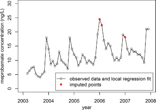
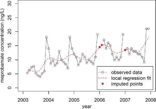
Helpful hint: The imputation of the missing data points presents an excellent opportunity to let students make a difficult decision and justify it. If one uses more customary values for the span and degree (e.g., 0.2 and 1), the chemical time series is fit with a smooth curve (Figure 6). Students can rightly argue that they have no way of knowing what the chemical concentrations would have been had water samples been collected and analyzed during the three missing months in 2006 and 2007 and thus using values cited by Cleveland (1979) is a reasonable approach. Additionally, values of the span less than 0.11 lead to values for the missing 2006 data that exceed all other values in the chemical time series. An argument can be made that one should not use imputed values that fall outside the range of observed values since there is no basis in the dataset for concentrations of that magnitude in water samples from Lake Mead. However, fitting the dataset with the loess and predict commands only leads fitted data to match observed data when the span and degree equal 0.08 and 2, respectively. Thus, one can also argue that using the imputed data that exceed observed values (Figure 5) is appropriate because the modeled data match the observed data exactly. This dilemma allows the instructor to reinforce that statistics is often about judgment and critical thinking. The author allows students to continue with their assignments using any imputation of the missing datum points so long as they can explain and defend their choice.

Figure 6. Observed data from Benotti et al. (2010) and local regression fit, which used a span of 0.2 and a degree of 1.

3.3. Research Task 3: Decomposition of the Chemical Time Series

Seasonal time series can be decomposed into a seasonal component, a long-term trend component, and a remainder. The seasonal component consists of repeated cyclic variation in the data that occurs with a regular frequency (in this case, yearly). The long-term trend component consists of variation that is nonstationary and either noncyclic or cyclic at low frequencies. The remainder component is a time series of remainders generated when the summed seasonal and long-term trend components are subtracted from the observed data. Decompositions can be performed using the stl command in R, which was developed by Cleveland et al. (1990). An abbreviation for “seasonal-trend decomposition procedure based on loess,” stl uses local regression to create a smoothed curve for the seasonal trend, which is then removed from the observed data so that a smoothed curve can be created for the long-term trend. This procedure is iterated until remainders are minimized. The decompose command, which uses moving averages, is also available in R, but the author prefers to use the stl command when teaching because its implementation in R is based on a single research paper that can be given to students (Cleveland et al. 1990). Additionally, stl is based on local regression, and thus it can be used to show an advanced application of that topic after introducing it as described above. It is also regarded as a superior decomposition method relative to methods known as “classical decomposition” and “X-12-ARIMA” (Hyndman and Athanasopoulos 2015).

Before decomposing the chemical time series, the imputed values must be inserted into it. This is easily done with the R commands

chemicals.int←chemicalschemicals.int[35,“meprobamate”]←chemicals.pred[35]

and similar for rows 36 and 47. The stl command only accepts objects of class “time series,” which are created with the ts command. The ts command accepts an array that is part of a matrix (the chemical dataset must be coerced to an object of class “matrix”), a starting time, and the number of observations per unit time. As such, the starting time of this dataset should be entered as a year expressed as a floating-point number (i.e., 2003.167 for March 2003). Sample code is

An object of class time series is accepted by the stl command along with a range of arguments that specify the window sizes and degrees of the local regressions that determine the seasonal component, long-term component, and other details. The argument s.window, which specifies the window for the seasonal component, has no default. If a value for the argument t.window, the window size for the long-term trend component, is not specified, its default is$\text{t}.\text{window} \ge \frac{1.5\cdot \text{frequency}}{1-\frac{1.5}{\text{s}.\text{window}}}$where t.window is selected as the smallest odd integer that fulfills the inequality (Cleveland 1990). This relationship between t.window and s.window ensures that the two components of the time series decomposition do not compete for variation in the time series data (Cleveland et al. 1990). Thus, the selection of s.window is often used to specify the windows for both components of the time series. In the Benotti et al. (2010) chemical time series, t.window converges on 19 time steps (i.e., months) for all s.window values above 29, so this value of s.window is appropriate. The stl command produces an object of class “stl,” and using the object name as an argument in a plot command produces a plot that shows the observed data, the seasonal component, the long-term trend component, and the remainder as time series in four panels (Figure 7). Commands in R for this time series decomposition are

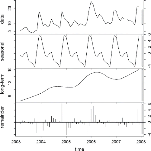
Figure 7. Four-panel decomposition plot of chemical time series data. Top panel: Observed data with interpolated points replacing missing values. Second panel: Seasonal component. Third panel: Long-term trend component. Bottom panel: Remainder. Units of vertical axes are ng/L, and gray bars indicate relative scale between the panels.

chemicals.stl<-stl(chemicals.ts,s.window = 29)

plot(chemicals.stl)

An object of class “stl” contains multiple elements. One is a matrix called “time.series” that contains “seasonal,” “trend,” and “remainder” columns that hold objects of class “ts.” This allows for easy isolation and plotting of the data that comprise the four-panel decomposition plot.

To assess the goodness of fit of a time series decomposition, the long-term trend component and the seasonal component can be summed and regarded as a statistical model for the observed time series data. Then, this model can be regressed against the observed data and the coefficient of determination reported. Sample code is

and the value of the resulting R² is 0.81. Environmental data frequently contain unpredictable variability, and so a model of the chemical time series data that describes more than 80% of the observed variability is acceptable for continuation of the exploration of this dataset. The complete R code for this time series decomposition appears in the appendix available in the SI.

Helpful hint: Procedures in this section can be scaled to fit an instructor's course plan and students' interests and aptitudes. The s.window argument can be provided to students without discussion (this has been the author's practice), or students can be asked to read the paper by Cleveland et al. (1990), demonstrate an understanding of the relationship between s.window and t.window, experiment with multiple values for each argument, and defend a choice. Similarly, assessment of goodness of fit can be neglected or this step can be used to reinforce the notion to students that executing a series of commands without error messages does not imply completion of a statistical analysis. The author asks his students to invent a goodness-of-fit metric for the time series. Assessment of goodness of fit is also useful because it requires extraction of elements of an object of class “stl.” This skill will be necessary later in this exercise.

Decomposition of the chemical time series yields a seasonal component with a minimum in October, a sharp rise through November to a peak in December, and then a decreasing trend during spring, summer, and autumn that is interrupted by a local maximum in May and June (Figure 7). The long-term trend component shows an overall increase in meprobamate concentrations between 2003 and 2008. While generally consistent with the findings of Benotti et al. (2010), this is interrupted by a period of relatively invariant concentrations from mid-2004 to early summer 2005 and a decrease in late 2006. The seasonal and long-term trend components both vary on a scale that is about half as large as the range of the observed data. The magnitude of the remainder component tends to be larger in winter than in summer. Analysis of the long-term trend component appears in Section 3.4. Observations related to the seasonal and remainder components are discussed in Section 3.5.

3.4. Research Task 4: Evaluation of Dilution as a Mechanism for the Long-Term Chemical Trend

Isolation of long-term trends of the volume of Lake Mead and the chemical time series allows for a rigorous investigation of the claim made by Benotti at al. (2010) that volume and chemicals are inversely related due to dilution. After reservoir volume data are read in from the data file “Lake_Mead_volume_SC_elevation_time_series_monthly.csv,” decomposition of the volume time series is analogous to the decomposition described above for the chemical time series. The results of this decomposition create a model that describes the observed data with a coefficient of determination of 0.97.

Alternative application: To create the monthly dataset of volume and SC data for Lake Mead, daily volume data and SC data collected approximately weekly were downloaded from the SNWA (2011). Local regression was then used to interpolate SC data to create a daily time series. Then, monthly means were taken for both variables. The daily dataset (“Lake_Mead_volume_SC_time_series_daily.csv”) has been included so that students can practice coding the conceptually simple operation of tabulating monthly means to generate this time series for themselves. Sample code (Section 4.2 of the appendix available in the SI) involves nested loops and an if-then-else-if-else statement.

Comparison of the long-term trends of the chemical and reservoir volume time series can be facilitated with an overlay plot (Figure 8). This requires plotting the “trend” time series in the “time.series” element of each object produced by the time series decomposition. Sample code for one of the trends is as follows:

Figure 8. Comparison of meprobamate concentration and volume of Lake Mead. Left: Overlay plot of long-term trend components of time series decompositions. Right: Plot of long-term trend of chemicals versus volume of Lake Mead.

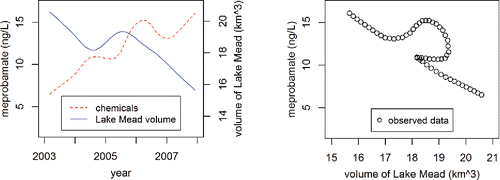
Although Benotti et al. (2010) based their claims on separate depictions of time series of chemicals and lake level, showing these separately or creating the overlay plot shown in the left panel of Figure 8 does not directly assess the relationship between these two variables. When plotted against one another (right panel of Figure 8), the resulting plot is nonlinear because, when the volume of Lake Mead was rising during 2004 and 2005 at roughly the same rate at which it had been falling at the beginning of the time series, meprobamate concentrations did not drop at the same rate as they had been rising early in the time series (left panel of Figure 8). Additionally, meprobamate concentrations fell in 2006 despite falling reservoir volume. At the beginning and the end of the time series, these long-term trends were linearly and inversely related (right panel of Figure 8). Consequently, time series decomposition shows that the long-term claims made by Benotti et al. (2010) hold for parts but not all of the dataset.

Potential pitfall: Plotting one time series versus another as a scatterplot generates a plot in which the values of the time points of the time series (e.g., 2003.167 and 2003.250) are used as markers. A visually attractive scatterplot can be created by coercing the long-term trend components of the two time series decompositions to objects of class “numeric.” Sample code for the long-term trend component of the chemical time series is as follows:

chemicals.trend<-as.numeric(chemicals.stl$time.series[,“trend”])

Alternative application: This exercise can also be completed using water surface elevation instead of volume. Because Lake Mead is a reservoir constructed on a major river, it experiences a net flow from its upstream end toward its dam. Perceptive students may realize that, when chemicals enter Lake Mead at its downstream end near Las Vegas, their complete circulation throughout this maximum of 190-km-long reservoir is virtually impossible. Only the volume of Boulder Basin, the basin between a narrow section of Lake Mead and Hoover Dam into which Las Vegas Wash discharges, is relevant for dilution of wastewater chemicals. The use of the volume of Lake Mead to evaluate the claims of Benotti et al. (2010) is based on the assumption that a fractional decrease in the volume of the entire reservoir implies an approximately similar fractional decrease in the volume of Boulder Basin. Refining this assumption and testing the assumption that chemicals might mix completely in Boulder Basin over time scales of many months is a lake science question that is beyond the scope of this exercise. Much progress on these topics has been made using three-dimensional hydrodynamic modeling (Preston et al. 2014a, 2014b). If the instructor or students are uncomfortable with the assumption that relative volume changes of Boulder Basin will mirror those of Lake Mead or that chemicals will mix throughout Boulder Basin as they reach the sampling point at its bottom, the evaluation of the claims of Benotti et al. (2010) can be done using the lake elevation time series included in “Lake_Mead_volume_SC_elevation_time_series_monthly.csv.”

3.5. Research Task 5: Evaluating Seasonal Influences on the Chemical Time Series

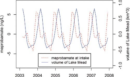
Time series decomposition allows exploration of the seasonality of the chemical time series. An overlay plot of the seasonal components of the chemical and volume time series, which can be created similarly to the overlay plot of the long-term trend components (see above), indicates that seasonal minima in meprobamate slightly lag seasonal minima in reservoir volume. Also, seasonal maxima in meprobamate precede by two months seasonal maxima in reservoir volume (Figure 9). Intuition suggests that, if dilution is an important influence on seasonal variation of wastewater-derived chemicals in Lake Mead, its effect would occur immediately or after a delay of a couple months. This can be evaluated efficiently using cross-correlation, which computes the Pearson's correlation coefficient of one time series lagged relative to another. The command in R is “ccf”; sample code is as follows:

Figure 9. Seasonal components of chemical time series and volume of Lake Mead.

where

·	“meadvol.stl” is the object to which the time series decomposition of the volume time series was assigned (R code for this command is not shown),
·	the “lag.max” argument specifies the number of time steps to lag the first time series relative to the second,
·	the “plot = F” suppresses the automatically generated plot that occurs as a default, and
·	the second and third commands assemble a table of lags and correlation coefficients.

Complete R code for this step appears in the SI.

With no lag, the Pearson's correlation coefficient between the seasonal components of these two time series is 0.30 (Table 1). If dilution were an important mechanism controlling chemical concentrations on a seasonal time scale, then one would expect large-magnitude, negative correlations with lags of 0, 1, or 2 month(s). Instead, these values are 0.09 and −0.03 for lags of 1 and 2 month(s), respectively (Table 1), indicating no correlation between these variables and invalidating this explanation for meprobamate concentrations.

Potential pitfall: The concept of lagging one time series relative to another can be difficult to conceptualize correctly. The above syntax indicates that the seasonal component of the chemical time series is lagged relative to the seasonal component of the volume time series. Thus, rather than calculating a Pearson's correlation coefficient where both seasonal components start in March 2003, a lag of 1 month implies that April 2003 to December 2007 of the seasonal component of the chemical time series is compared to March 2003 to November 2007 of the seasonal component of the volume time series. Ignoring the last month of the seasonal component of the volume time series is necessary, so that there are an equal number of values in each dataset, which is required for the calculation of a Pearson's correlation coefficient.

Potential pitfall: The novice student can visualize the lags in a cross-correlation analysis explicitly by copying the time series being compared into Microsoft Excel and executing the “correl” command multiple times. However, this will lead to slightly different results than those produced by R because the ccf command in R uses the total sum of squares (TSS) from the lag = 0 case in all calculations, whereas unique “correl” commands in Excel will each involve unique TSS values that will be different from the lag = 0 case. To make Excel calculations match those of R, it is necessary to calculate Pearson's correlation coefficients explicitly by determining in separate commands the sums of squares and the TSS value of the lag = 0 case so that it can be applied to all determinations of Pearson's correlation coefficient.

Alternate application: Interestingly, the cross-correlation function described above also yields moderate-to-high and positive Pearson's correlation coefficients of 0.57, 0.72, and 0.58 for negative lag values of 1, 2, and 3 month(s), respectively (Table 1). This occurs because these lags effect the alignment of the maxima of the two seasonal components (Figure 9). This is not indicative of dilution or another mechanism of hydrologic control of chemical concentrations because the maximum in chemicals precedes the maximum in water volume, and so the latter cannot affect the former if it happens later. Additionally, dilution implies an inverse rather than a direct correlation. The approximate temporal correlation of these two seasonal components results from a separate influence on both datasets. In early winter, chemical concentrations at the SNWA drinking water intake reach their yearly maximum because of lake circulation processes that are described below. In late winter each year, the reservoir volume peaks because steady inflows from an upstream reservoir refill Lake Mead after the discontinuation of agricultural irrigation each autumn. So, the onset of winter induces both the enrichment of chemicals in the deep water of Lake Mead and the refilling of the reservoir, and so the respective seasonal components peak a couple months apart. This can be shown to students as an instance in which correlation does not imply causation. Not only is there no physical or chemical basis for the chemical maximum inducing the volume maximum or vice versa, but also a separate influence exists that influences both these events separately.

Table 1. Cross-correlation analysis of seasonal component of chemical time series lagged against seasonal component of Lake Mead volume time series.

Lag^a	r^b
−3	−0.58
−2	−0.72
−1	−0.57
−0	−0.30
1	−0.09
2	−0.03
3	−0.20

^a Lag is expressed in time steps (i.e., months).

^b Pearson's correlation coefficient.

Comparison of the seasonal trend of the chemical time series with the seasonal trend of the SC time series provides an insight into the seasonality of chemicals in Lake Mead that linear regression of chemicals against volume (or water surface elevation) does not. Evaluation of SC has the pedagogical value of asking students to repeat the time series decomposition and analysis described here from start to finish. It will reward those who have created an organized and well documented script in R. Only minor modifications to the exercise as described above are needed to read in the SC time series, conduct a time series decomposition, isolate the seasonal component, create an overlay plot with the seasonal component of the chemical time series, and conduct a cross-correlation analysis. The results of this decomposition create a model that describes the observed data with a coefficient of determination of 0.97. Results indicate substantial overlap between the seasonal components of the SC and chemical time series (Figure 10). The Pearson's correlation coefficient of largest magnitude is 0.89, and it occurs at lag = 0. Because elevated SC is an indication of the presence of treated-wastewater-rich water from Las Vegas Wash at the SNWA drinking water intake, this comparison shows, unsurprisingly, that seasonal variation in WDOCs at the bottom of Lake Mead tracks closely with the presence of wastewater there.

Figure 10. Seasonal components of chemical time series and specific conductance measured at the location of water sampling at the bottom of Lake Mead.

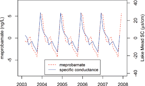
The seasonal variation in SC at the bottom of Lake Mead depends on circulation patterns that are described in detail elsewhere (e.g., LaBounty and Burns 2005; Preston et al. 2014b). Two of these circulation patterns are most important. The wintertime deepening of the thermocline (i.e., the boundary between warm surface water that is mixed by wind and colder deep water that is isolated from the atmosphere) reaches the bottom of Lake Mead approximately every other year (LaBounty and Burns 2007). When the temperature of the water of Las Vegas Wash, which is rich in treated wastewater, differs from that of Lake Mead, the inflowing water of Las Vegas Wash will float on top of Lake Mead water or plunge to the bottom of the reservoir. The former occurs in spring and early summer when the wash has warmed more rapidly than the reservoir, and the latter occurs in autumn and early winter when the wash has cooled more rapidly than the reservoir (Preston et al. 2014b). While these processes are seasonal, their timings and magnitudes are not consistent between years and they are most uncertain in winter. This implies that the magnitudes of the peaks of wastewater at the SNWA drinking water intake will vary slightly between years and thus will not be perfectly represented by the seasonal component of a time series decomposition. This explains the increase in the remainder component for the decomposition of the chemical time series (Figure 7) in some winters.

4. Discussion

This exercise is a part of one of the five “technical assignments” in the author's data science course, and students regard it as the most difficult and technically demanding. Before the assignment is due, 8.5 hr of class time give the students background and practice as preparation for this exercise. The Benotti et al. (2010) paper is explained and reviewed so that the motivation for the assignment is clear, the nature and significance of time series concepts (i.e., basic characteristics and types, autocorrelation, decomposition, detrending, and forecasting) are introduced and discussed, and the commands loess, ts, stl, and acf are introduced in small-group activities with the instructor present. In the assignment, students are asked in separate questions to explain major features of the sample local regression script by Glynn (2005), to impute missing data with local regression (i.e., Research Task 2), and to comment on how well the arguments of Benotti et al. (2010) hold for the long-term and for seasonal trends after decomposing the chemical and elevation time series and performing a cross-correlation analysis (i.e., Research Tasks 3 and 4). Development of a goodness-of-fit metric is optional. Each of these questions is graded out of 10 points, and the maximum score for an incorrect answer is generally 6 out of 10 points when core concepts are demonstrated well. After the graded assignment is returned to them, students have the opportunity to correct their mistakes in response to feedback received and thus earn higher grades.

This exercise presents multiple opportunities for expansion for well-prepared audiences. The author considers the core of the exercise to be Research Tasks 2–4 because they capture the bulk of its statistical thinking (see below). The exercise can be expanded by preceding the Research Tasks with independent reviews of the Benotti et al. (2010) paper and generation of a proposed list of research tasks. Additionally, students could read the papers by Cleveland (1979) and Cleveland et al. (1990) and explain in their own words the details of local regression and time series decomposition before the background in Sections 3.2 and 3.3 is presented to them. The invention of a goodness-of-fit metric could be mandatory. Students could be given only the daily time series for the SC and volume datasets, and they could make the monthly datasets themselves.

This exercise can also be contracted in several ways to suit audience abilities. Hint sheets could be provided to students to list useful commands and their syntax. Students could be notified of the potential pitfalls that appear in this article. Research Task 1, which serves as a skills warmup, or Research Task 5, which provides closure to motivation for the exercise, could be led by the instructor or omitted entirely. Finally, answers or important figures could be provided for students to reproduce so that they know they are moving in the right direction while making decisions and coding.

This investigation allows students to use multiple statistical tools (primarily local regression, time series decomposition, and cross-correlation) to evaluate in detail a real water-quality dataset from a major water-supply reservoir. It shows how much more richness can be explored in a dataset past the linear regressions that are easy to perform in Microsoft Excel yet inappropriate for time series analysis. As such, it aligns with several recommendations of the Guidelines for Assessment and Instruction in Statistics Education (GAISE) College Report 2016 (GAISE College Report ASA Revision Committee 2016). It teaches statistical thinking by asking students to be thoughtful consumers of the data analysis by Benotti et al. (2010), by allowing students the opportunity to design the investigative process, and by requiring that students use statistical techniques in a problem-solving context. Additionally, the graphing required is important for the interpretation of the results, and, once a student's R code works, critical thinking is required to evaluate output and make original claims. This exercise focuses on conceptual understanding because it explains the underlying rationale and shows the mathematical formulations for the loess and stl commands. It integrates real data with a clear context and a statistically meaningful purpose. It fosters active learning because its complexity requires careful engagement and because students will benefit from group work and contact with their instructor. Finally, it uses assessment to improve student learning because formative feedback is provided to students as they work through a sequence of research tasks designed to help deepen their understanding of time series.

This exercise stops short of introducing students to forecasting, although classroom activities or assignments where the goal is to predict chemical concentrations, for instance, could easily be built using these data. Also, lake level data are readily accessible (USBR 2011c) to evaluate prediction accuracy.

Supplementary Materials

Complete R code for this exercise is available as appendix, which can be accessed on the publisher's website.

Acknowledgments

Todd Tietjen and Peggy Roefer of the SNWA provided helpful discussion and database access, respectively. Glen van Brummelen and Jim Cohn (Quest University Canada) created the opportunity for the author to teach the statistics course in which this exercise was developed. Lucas Nguyen (Quest and Geosyntec Consultants, Inc.) made early contributions toward analyses of the chemical dataset. Lonnie Wake (Quest) provided helpful discussion at key points during conceptual development of this manuscript. The comments of Editor Dr. Bethany White and two anonymous reviewers allowed substantive improvements to the first version of the manuscript.

Funding

Part of this work was supported by a French Environmental Fellowship awarded to the author through the Harvard University Center for the Environment.

References

- Barnes, K. K., Kolpin, D. W., Furlong, E. T., Zaugg, S. D., Meyer, M. T., and Barber, L. B. (2008), “A National Reconnaissance of Pharmaceuticals and Other Organic Wastewater Contaminants in the United States – I) Groundwater,” Science of the Total Environment, 402, 192–200.
- Barnett, T. P., and Pierce, D. W. (2008), “When Will Lake Mead Go Dry?” Water Resources Research, 44, W03201.
- Benotti, M. J., Trenholm, R. A., Vanderford, B. J., Holady, J. C., Stanford, B. D., and Snyder, S. A. (2009), “Pharmaceuticals and Endocrine Disrupting Compounds in U.S. Drinking Water,” Environmental Science and Technology, 43, 597–603.
- Benotti, M. J., Stanford, B. D., and Snyder, S. A. (2010), “Impact of Drought on Wastewater Contaminants in an Urban Water Supply,” Journal of Environmental Quality, 39, 1196–1200.
- Bruce, G. M., Pleus, R. C., and Snyder, S. A. (2010), “Toxicological Relevance of Pharmaceuticals in Drinking Water,” Environmental Science and Technology, 44, 5619–5626.
- Cleveland, R. B., Cleveland, W. S., McRae, J. E., and Terpenning, I. (1990), “STL: A Seasonal-Trend Decomposition Procedure Based on Loess,” Journal of Official Statistics, 6, 3–33.
- Cleveland, W. S. (1979), “Robust Locally Weighted Regression and Smoothing Scatterplots,” Journal of the American Statistical Association, 74, 829–836.
- Colborn, T., Dumanoski, D., and Meyers, J.P. (1997), Our Stolen Future, New York, NY: Plume.
- Focazio, M. J., Kolpin, D. W., Barnes, K. K., Furlong, E. T., Meyer, M. T., Zaugg, S. D., Barber, L. B., and Thurman, M. E. (2008), “A National Reconnaissance for Pharmaceuticals and Other Organic Wastewater Contaminants in the United States – II) Untreated Drinking Water Sources,” Science of the Total Environment, 402, 201–216.
- GAISE College Report ASA Revision Committee (2016), Guidelines for Assessment and Instruction in Statistics Education College Report 2016, Alexandria, VA: American Statistical Association. Available at http://www.amstat.org/education/gaise.
- Glynn, E. F. (2005), “loess Smoothing and Data Imputation,” Stowers Institute for Medical Research [online]. Available at http://research.stowers-institute.org/efg/R/Statistics/loess.htm.
- Hyndman, R. J., and Athanasopoulos, G. (2015), Forecasting: Principles and Practice, O-Texts: Online, Open-Access Textbooks [online]. Available at https://www.otexts.org/fpp.
- Kümmerer, K. (2010), “Pharmaceuticals in the Environment,” Annual Reviews of Environment and Resources, 35, 57–75.
- LaBounty, J. F. and Burns, N. M. (2005), “Characterization of Boulder Basin, Lake Mead, Nevada-Arizona, USA–Based on Analysis of 34 Limnological Parameters,” Lake and Reservoir Management, 21, 277–307.
- ———. (2007), “Long-Term Increases in Oxygen Depletion in the Bottom of Waters of Boulder Basin, Lake Mead, Nevada-Arizona, USA,” Lake and Reservoir Management, 23, 69–82.
- MacDonnell, L. J. (2009), “Colorado River Basin,” Water and Water Rights, 4, 5–54.
- Preston, A., Hannoun, I. A., List, E. J., and Tietjen, T. (2014a), “Three-Dimensional Management Model for Lake Mead, Nevada, Part 1: Model Calibration and Validation,” Lake and Reservoir Management, 30, 285–302.
- Preston, A., Hannoun, I. A., List, E. J., Rackley, I., and Tietjen, T. (2014b), “Three-dimensional management model for Lake Mead, Nevada, Part 2: Findings and Applications,” Lake and Reservoir Management, 30, 303–319.
- R Core Team (2014), R: A Language and Environment for Statistical Computing, R Foundation for Statistical Computing, Vienna, Austria: Author. Available at http://www.R-project.org/.
- ———. (2015), “Local Polynomial Regression Fitting,” R Stats Package Documentation, [online]. Available at https://stat.ethz.ch/R-manual/R-devel/library/stats/html/loess.html.
- Schwarzenbach, R. P., Escher, B. I., Fenner, K., Hofstetter, T. B., Johnson, C. A., von Gunten, U., and Wehrli, B. (2006), “The Challenge of Micropollutants in Aquatic Systems,” Science, 313, 1072–1077.
- Sedlak, D. (2014), Water 4.0: The Past, Present, and Future of the World's Most Vital Resource, New Haven, CT: Yale University Press.
- Southern Nevada Water Authority. (2011), “SNWA Members” [online]. Available at http://www.snwawatershed.org/members.
- United States Bureau of Reclamation (USBR) (2011a), “Colorado River Basin Water Supply and Demand Study, Interim Report No. 1,” Washington, D.C.: U.S. Department of the Interior.
- ———. (2011b), “Lake Mead Area and Capacity Tables,” [online], Washington, D.C.: U.S. Department of the Interior. Available at http://www.usbr.lc/region/g4000/LM_AreaCapacityTables2009.pdf.
- ———. (2011c), “Lower Colorado Region: Daily Reservoir Elevation Archives,” [online]. Available at http://www.usbr.gov/lc/region/g4000/archives.cfm.
- Webb, R. H., McCabe, G. H., Hereford, R., and Wilkowske, C. (2004), “Climate Fluctuations, Drought, and Flow in the Colorado River Basin,” U.S. Geological Survey Fact Sheet, 2004–3062.
- Yafee, R. A., and McGee, M. (2000), Introduction to Time Series Analysis and Forecasting: with Applications of SAS and SPSS, San Diego: Academic Press.