Using Financial Investment Measures to Proactively Engage Students in the Introductory Business Statistics Course

ABSTRACT

Typically, the core-required undergraduate business statistics course covers a broad spectrum of topics with applications pertaining to all functional areas of business. The recently updated American Statistical Association's GAISE (Guidelines for Assessment and Instruction in Statistics Education) College Report once again stresses the pedagogical importance of topic and application relevancy in an increasingly data-centered world. To this end, only two introductory textbooks have incorporated some financial investment measures (Sharpe ratio and beta coefficient) in the teaching of numerical descriptive measures and simple linear regression analysis, respectively, while a few others include them as real-data application exercises at the end of their respective chapters. Although this latter coverage is in compliance with GAISE College Report recommendations on the importance of using relevant real data applications in the teaching of introductory business statistics, it forgoes an opportunity to provide more detailed discussion within the text itself and add value to a business student's learning. Given that all business students will have an opportunity to learn about financial investment, regardless of their functional area major, this paper offers a more proactive use of these and other financial investment measures as part of the current, traditional course or as part of a suggested dedicated introductory business statistics course for finance majors.

KEYWORDS:

• Alpha and beta coefficients
• Bootstrap percentile confidence interval
• Capital asset pricing model
• GAISE
• Permutation test
• Resampling method
• Sharpe ratio
• Simulation-based inference
• Treynor ratio

1. Introduction

The introductory business statistics course is given early in an undergraduate business school curriculum because it serves to support the functional disciplines of accountancy, finance, management, and marketing. Therefore, students enrolled in the business statistics course typically have no prior exposure to the functional business disciplines and, at most, have limited exposure to general business topics. At this early point in the educational process, these undergraduate students can only aspire to become accountants, financial analysts, managers, and marketing leaders. Therefore, when preparing to teach the introductory business statistics course, instructors need to take this into account in their selection of textbook and choice of classroom applications and assignments. Appropriately selected applications and assignments can inspire or engage students in connections with their selected disciplines. For those who have not yet declared a discipline specialization, the classroom applications and assignments should at least be realistic, if not real, and they must be appealing so that they have the potential for sparking student interest in a particular discipline.

The recent updates to the American Statistical Association's GAISE (Guidelines for Assessment and Instruction in Statistics Education) College Report (Aliaga et al. 2005) once again stress the pedagogical importance of topic and application relevancy in an increasingly data-centered world (Carver et al. 2016; Everson and Mocko 2015a, 2015b). In the present learning paradigm, not only must they be relevant, the student audience must see them as so.

According to the business school accrediting body AACSB International, concentrations, majors, or tracks in finance, one of the more quantitative functional disciplines, currently constitute 10.5% of all its accredited programs (Mondello 2015) but the percentage of undergraduates pursuing this particular discipline is believed to be higher. For example, at this campus, finance is one of 17 concentrations in the business school, but currently finance majors comprise 15.1% of all declared business major enrollments.

Appropriately, a few textbooks developed to support the traditional business statistics courses (Stine and Foster 2011; Jaggia and Kelly 2013) have incorporated some financial investment measures (Sharpe ratio and beta coefficient) in the teaching of numerical descriptive measures and simple linear regression analysis. In a few other texts, these measures appear as real-data application exercises at the end of their respective chapters. Although this latter coverage is in compliance with GAISE College Report recommendations, a more inclusive approach can add value to business students' learning.

Given that all business students will have an opportunity to learn about financial investment, regardless of their functional major, we recommend a more proactive use of the Sharpe ratio and beta coefficient along with two other important financial investment measures, the alpha coefficient and the Treynor ratio (see Section 2), either as part of the current traditional business statistics course or, as suggested here (see Section 6), as part of a dedicated introductory statistics course for finance majors.

The remainder of this article is divided into five sections. Section 2 provides a brief overview of financial investment and describes the four measures we suggest including in both traditional and dedicated course offerings. Section 3 on pedagogical implications provides a summary of the six key recommendations of the GAISE College Report in support of this approach for such courses and also contains a literature review on the pedagogical advantages of using resampling methods in such courses. Section 4 discusses the importance of developing conceptual understanding, addresses a dilemma in teaching and student learning, and stresses the benefit of introducing resampling methods into the business statistics curriculum. Section 5 presents an application employing resampling methods to actual data from two companies to demonstrate how these can be used in dedicated courses. Section 6 suggests how the four financial investment measures can be best taught to an introductory business statistics audience – either in a traditional or dedicated course setting. Appendix A provides a brief summary of the various relationships among the four financial investment measures. Appendix B is an overview of resampling methods—bootstrap estimation and permutation testing – two components of simulation-based inference. Appendix C describes how the bootstrap and permutation distributions are generated using Excel. The appendices are available in the online supplementary material.

2. Financial Investment: An Overview

A good overview of modern investment theory is found in Bernstein's 1992 book Capital Ideas: The Improbable Origins of Modern Wall Street.

How to identify the appropriate risk to evaluate equity investments was a long-standing problem for investors. Modern finance theorists began a systematic assault on this issue in the 1950s and the seminal insight in the field was the development of modern portfolio theory by Markowitz (1952, 1959). He recognized that investors need to diversify their holdings to avoid undue risk.

The next problem was the appropriate risk metric for an individual company's stock in this setting. The solution was the now famous capital asset pricing model (CAPM) developed simultaneously and independently by Sharpe (1964), Lintner (1965), and Mossin (1966). They proposed that the “beta” is the appropriate measure of a company's “systematic” risk in a large, well-diversified portfolio. The CAPM is presented in finance textbooks (e.g., Ross, Westerfield, and Jordan 2016) as$R_s=R_f+{\beta }_s(R_M-R_f),$where $R_s$ is the estimated long-term return on a stock, $R_f$ is the return on the “risk-free asset,” $R_M$ is the return on the market portfolio, $(R_M-R_f)$ is the “excess return on the market,” that is, the average extra return received for investing in the risky market above the return received for the risk-free asset, and ${\beta }_s$ is the slope, showing how the returns on a company's stock vary against the market portfolio. Within the CAPM framework ${\beta }_s$ is the measure of systematic risk, which should solely explain the return on a stock given its relevant risk.

In practice, beta for a company is usually estimated using the market model, regressing the periodic return on the asset against that for a representative large, well-diversified portfolio as follows:${\hat{Y}}_i=\hat{\alpha }+{\hat{\beta }}_s{X}_i,$where $X_i=R_{M_i}$ is the return on the market portfolio in period i and $\hat{\alpha }$ is the estimate of the intercept of the regression model. In his derivation, Sharpe notes that the alpha in this model should be 0.

This leaves the issue of assessing the risk-based return for a company. There are three widely-used methods. Treynor (1966) suggests a comparison of the excess return on the company's stock to its beta. Sharpe (1966) recommends a similar approach, but compares the return to the standard deviation rather than beta. Jensen (1968), however, notes that beta should capture all of the relevant return. This implies that when the alpha estimated in the market model is statistically significantly different from 0, a company is over or under performing for its intrinsic risk (depending upon whether it is positive or negative).

The CAPM is a very simple theoretical framework but there is no guidance on how it should be used in practice. Initially, there was some suspicion about the approach among practitioners in both the investment community and in corporate finance. They questioned whether it should be used and how to estimate the required variables. However, a well-referenced survey of corporate executives by Graham and Harvey (2002) indicates that a majority of managers commonly use the approach to estimate their firms' costs-of-capital. Regardless, since its inception the CAPM has been a mainstay in finance courses.

Business majors are normally introduced to the CAPM in the introductory finance course, so that having some familiarity with the concept and the related financial investment measures from the introductory statistics course will prepare them for a more thorough discussion in their finance course. Therefore, the four easy-to-use financial investment measures (Jordan and Miller 2012) described here in the sequence which appears to be most appropriate for teaching are the Sharpe ratio, the beta coefficient, the alpha coefficient, and the Treynor ratio.

As developed in the Jaggia and Kelly (2013) text, it makes sense to present the Sharpe ratio following the discussion on numerical descriptive measures. Its use here is consistent with the desire to inspire students with relevant material and show them how descriptive statistical measures are used in practice. In this text and in the Stine and Foster (2011) text, the beta coefficient and the alpha coefficient are presented as part of the development of the simple linear regression model. The Treynor ratio is dependent upon the beta coefficient so this concept must be taught last.

2.1. The Sharpe Ratio

The Sharpe ratio measures how well the return of an investment compensates for the risk that is being taken. When comparing two or more potential investments the one with the highest Sharpe ratio has provided the best return for the underlying risk taken.

The Sharpe ratio is obtained using a set of time-series data on the percentage change from one period to another. The mean and standard deviation of these percentage changes are computed.

The Sharpe ratio for a particular investment is given by$\text{Sharpe ratio}=\frac{\overline{Y}-R_f}{S_Y},$where $\overline{Y}$ is the mean return for the particular investment (in percent), $S_Y$ is the standard deviation for the investment (in percent) and $R_f$ is the constant return for a risk-free investment such as a savings account (in percent).

The numerator of the Sharpe ratio measures the extra reward that an investor would receive for the added risk taken—this difference is called excess return. The ratio is this excess return divided by the standard deviation. The higher the Sharpe ratio, the better the investment compensates the investor for the risk taken.

2.2. The Beta Coefficient

The beta coefficient is a measure of the volatility of a stock. It is obtained by developing a simple linear regression model using the monthly percentage changes in the stock price as the dependent variable and the corresponding percentage changes in a market index such as the Standard & Poors Index of 500 Stocks (hereafter referred to as S&P 500) as the independent variable. The slope of the fitted sample regression equation is the beta coefficient. Therefore,

Predicted monthly percentage change in a stock's price = $\hat{\alpha }+{\hat{\beta }}_s$ (monthly percentage change in S&P 500), where ${\hat{\beta }}_s$, the sample slope, is the estimated beta coefficient for the stock.

Note that the market is attributed a beta coefficient of 1, so that a stock with a slope of +1 tends to move the same as the overall stock market. A stock with a beta coefficient greater than 1 has more systematic risk than the market average so a stock with a beta of +1.50 tends to move upward 50% more steeply than the overall stock market. On the other hand, a stock with a beta of +0.60 tends to move only 60% as much as the overall stock market. Moreover, stocks with negative slopes (i.e., negative beta values) tend to move in the opposite direction of the overall stock market.

The beta coefficient is often calculated in five or more years of monthly data or one year of weekly data.

2.3. The Alpha Coefficient

According to The Charles Schwab Corporation (2015), the beta coefficient “measures an investment risk in comparison to the market as a whole” while the alpha coefficient “measures the extra return on an investment over a benchmark.”

The alpha coefficient is obtained by developing a simple linear regression model using the monthly percentage changes in the stock price as the dependent variable and the monthly percentage changes in a market index such as the S&P 500 as the independent variable. The Y-intercept of the fitted sample regression equation is the alpha coefficient. From the above sample linear regression model $\hat{\alpha }$ is the Y-intercept, or alpha coefficient—the average percentage change in the price of a share when the market is flat, that is, showing a 0% change. Sharpe (1964) demonstrated that the alpha in the market model should be 0 if assets are priced efficiently in the market (beta alone should explain security returns). Therefore, if the alpha coefficient is statistically significantly different from 0, this suggests that the return on the asset has been abnormally high or low for the amount of (systematic) risk taken. This is why Jensen (1968) argued that alpha is the best measure of a firm's market performance. For instance, if the alpha coefficient is −0.25, the return for the security is a quarter of a percent lower over the time-period studied than is expected for a stock having its particular beta coefficient.

2.4. The Treynor Ratio

The Treynor ratio measures how well the return on an investment compensates for the systematic risk taken. When comparing two or more potential investments the one with the highest Treynor ratio has provided the best return for its beta.

The Treynor ratio is obtained using a set of data over time pertaining to closing price of a stock that indicates percentage change (i.e., growth) from one period to another and is also based on the beta coefficient obtained from a sample regression equation that predicts average percentage change in the price of a stock per unit percentage change in an overall market index.

The Treynor ratio for a particular investment is given by$\text{Treynor ratio}=\frac{\overline{Y}-R_f}{{\hat{\beta }}_s},$where $\overline{Y}$ is the mean return for the particular investment (in percent), $R_f$ is the constant return for a risk-free investment such as a savings account (in percent) and ${\hat{\beta }}_s$ is the beta coefficient or slope of the sample regression equation predicting average percentage change in the price of a stock per unit percentage change in an overall market index.

Similar to the Sharpe ratio, the numerator of the Treynor ratio measures the excess return. The ratio is this excess return divided by the beta coefficient. The higher the Treynor ratio, the better the investment is compensating the investor for the systematic risk taken.

2.5. Time-Series Data and Caveats

A time series is a set of numerical data collected over time, and business school students will typically use various time-series datasets in several of their courses. If first exposure to time-series data occurs in the introductory business statistics course, particularly with the kind of financial applications described herein, it is important that the students be aware of differences in such data compared to cross-sectional data obtained via a randomization process—be they from an experimental design in a course in biostatistics or from a random probability sample in a course in general applied statistics.

First, unlike data obtained from an experiment or survey, it would be unusual for a particular time-series dataset to be selected at random. Second, the sequence of numerical values in a time series will be time dependent; classical methods of statistical inference typically assume independence of selected sample observations. Third, time-series data are typically obtained for possible study of particular properties such as trend, seasonality, or cyclical behavior, or for purposes of forecasting data movements into the future. On the hand, when data are obtained from an experiment, typically inferential methods are used for drawing conclusions about differences due to treatment effects. And when data are obtained from a random probability survey, both descriptive and inferential methods are used for making decisions about population parameters based on observed sample statistics. Unless one is testing for randomness or pattern, time-series data are not amenable to inferential methods. Fourth, summary statistics such as the aforementioned financial investment measures computed from a time series are limited in meaning to the particular period for which the series is collected.

Further discussion on these issues is presented in Section 5.4.

3. Pedagogical Implications

In the re-engineering of this undergraduate, core-required introductory business statistics course with focus on enhancing proactive engagement, three key pedagogical issues must be addressed—what should be taught, why it should be taught, and where it should be taught. Once these issues are resolved the question becomes how the course should be taught.

The “what” and “why” are reflected in the course learning goals. A more appealing course will likely produce more motivated students who will be more proactively engaged, increasing opportunities for learning. The “where” makes the distinction between creating enhancements to a traditional course versus developing dedicated course sections for students intending to major in finance. The “how” focuses on mode of course delivery.

3.1. Employing the GAISE College Report Recommendations

Essential to this re-engineering process are the six key recommendations of the GAISE College Report displayed in Table 1.

Table 1. 2005 GAISE College Report Recommendations to enhance pedagogical delivery.

Recommendations
1–Emphasize statistical literacy and develop statistical thinking
2–Use real data
3–Stress conceptual understanding rather than mere knowledge of procedures
4–Foster active learning
5–Use technology to develop conceptual understanding and to analyze data
6–Use assessments to improve and evaluate learning

The following is a specific assessment on “what” and “why.” It reflects the purpose of this paper, that is, the use of financial investment measures to proactively engage students in the introductory business statistics course.

For more than a decade, aside from the texts by Jaggia and Kelly (2013) and Stein and Foster (2011), other major texts in introductory business statistics have, at best, only included the Sharpe ratio and, perhaps more likely, the beta coefficient as real data application exercises at the end of the respective chapters on numerical descriptive measures and simple linear regression analysis. Although, as shown in Table 1, such usage is aligned to the second GAISE College Report recommendation on the importance of having real data applications in the teaching of introductory business statistics, it seems to forgo an opportunity to provide greater value added to learning. Fortunately, the above-named texts include financial investment measures conceptually in the body of the text in addition to providing end-of-chapter problems. Applauding what these two texts have accomplished, we suggest how to further improve such pedagogy.

Jaggia and Kelly (2013) provided a brief but enlightening discussion of the Sharpe ratio immediately after introducing various descriptive measures for numerical variables. Conceptually, this seems to be where the topic belongs, particularly if the course and the text is intended for an undergraduate audience. On the other hand, Stein and Foster (2011) provided a really excellent discussion in a much later chapter, one that will probably not be addressed in the large majority of undergraduate level introductory courses (although positioned adequately for MBA courses). With respect to the Sharpe ratio, however, the latter text better distinguishes between concept and procedure–so important for enhancing pedagogy (see Table 1, Recommendation 3). The student audience must always be kept in mind. In defining the Sharpe ratio application Jaggia and Kelly (2013) used a T-bill as a risk free asset in the equation but Stein and Foster (2011) more appropriately employed a savings account for this purpose. Of course the T-bill is slightly less risky, but for students trying to learn statistical concepts and procedures before having had any real exposure to the subject of finance it seems better to use the savings account rather than an unfamiliar term.

Our intent here, however, is certainly not to be critical–the authors of these two texts should be applauded for attempting to put the Sharpe ratio application in the context of what has been learned about descriptive numerical measures, not placed only as an end-of-chapter exercise. Nevertheless, it seems here that pedagogy would be enhanced with the Stein–Foster (2011) presentation positioned in the Jaggia–Kelly (2013) setting.

With respect to beta coefficient applications, both texts give very good, appropriately positioned presentations in their chapters on simple linear regression. Their student audiences have an opportunity to see a real statistical application on real data important to financial investment decisions.

Expanding on these authors' achievements and guided by the GAISE College Report recommendations, we propose a more proactive use of the Sharpe ratio and beta coefficient along with the alpha coefficient and the Treynor ratio. This can be accomplished either as part of the traditional introductory business statistics course or, as will be suggested in Section 6, as part of a dedicated introductory business statistics course for finance majors. What will be essential to fully accomplish this, however, is to be able to introduce resampling methods into the curriculum of traditional business statistics courses or to be able to replace classical methods of statistical inference with resampling methods in the curriculum of dedicated statistics courses.

3.2. Including Resampling Methods in the Business Statistics Course Curriculum

The business statistics course is typically a prerequisite to the functional area courses and includes topics that serve the needs of these functional area courses. Given that classical methods of statistical inference have been engrained in the curriculum for half-a-century it has been difficult to introduce or replace these with resampling methods.

As discussed in Section 4.2, with modern computing technology resampling methods are now simple to execute. These methods are versatile and generally far more practical than traditional methods of classical inference which are dependent on stringent distributional assumptions. Therefore, the time has now come to include resampling methods in introductory business statistics courses.

The importance of introducing resampling methods into the teaching of statistics, regardless of the field of application, cannot be overemphasized. A review of the program from the Electronic Conference on the Teaching of Statistics (eCOTS 2016) indicates that both keynote speakers, 8 of 34 talks or panel discussions, and 6 of 33 poster sessions, that is, a total of 16 out of 69 sessions or 23.2%, discussed resampling methods.

Moreover, a review of statistical education publications over the past two decades indicates that resampling methods are gaining in popularity. These publications may be classified into three types—articles on educational philosophy, articles related to pedagogy and application (such as this one), and well-designed, innovative textbooks.

We find six recent thought-provoking articles pertaining to educational philosophy: Cobb (2007), Rossman and Chance (2008), Tintle et al. (2011), Cobb (2013), Forbes (2014), and Rossman and Cobb (2015).

Also related are 11 interesting articles pertaining to pedagogy and application: Simon and Bruce (1991), Simon (1994), Coakley (1996), del Mas, Garfield, and Chance (1999), Garrett and Nash (2001), Ernst (2004), Wood (2005), Chang et al. (2009), Ernst (2009), Eudey, Kerr, and Trumbo (2010), and Stephenson, Froelich, and Duckworth (2010).

In addition, three important texts stressing the approach have been published over the past few years: Rossman and Chance, 4th edition (2012), Lock et al. (2013), and Tintle et al. (2015). Appendix B provides an overview on resampling methods.

4. Developing Conceptual Understanding

To enhance pedagogy, the GAISE College Report recommends that only relevant data and examples be used when teaching a basic course, and that statistical software be used to assist in data analysis. This can be achieved by introducing the financial investment measures and then giving students practical assignments pertaining to specific companies. If students employ appropriate software it is not difficult to obtain the four chosen measures, but the real question is whether they have a conceptual understanding. The third recommendation in the GAISE College Report (see Table 1) stresses comprehension, not simply knowledge of the procedures. Robin Lock (August 2004), one of the authors of this GAISE College Report, said:

“If students don't understand concepts, there is little value in knowing procedures. If students do understand concepts, specific procedures are easier to learn.”

In order to develop conceptual understanding about these measures, students need to understand what their results convey, and appreciate what their numerical answers mean.

•	Is a company's Sharpe ratio of 0.40 good? Is it significantly better than a ratio of 0.35?
•	Is a company's beta coefficient of +1.28 too risky for most potential investors?

The bottom line: To develop comprehension students need to “feel” their data. And this pushes educators to reflect on what they have taught.

4.1. Addressing a Dilemma in Teaching and in Student Learning

Before introducing the Sharpe ratio students should be thoroughly exposed to visual/graphical presentations of both categorical and numerical data, including scatterplots and time-series plots. By that point, they should have studied descriptive statistical methods and understand, conceptually, what measures of central tendency, variation, shape, and peakedness convey. Moreover, students will also have some understanding of the sampling process and realize that every time a different random sample of size n is taken from a fixed population of size N, the items in the sample will differ, so the resulting statistics such as the mean and standard deviation will also differ—even though each of these sample statistics are providing estimates of their respective unknown population parameters.

If the intent of a classroom assignment is to have each student select and study only one company and compute its Sharpe ratio, then the pooled class results constitute a “sample” of company Sharpe ratios and the students would all have a dataset upon which they could perform a thorough descriptive analysis of this (sampling) distribution (of the Sharpe ratios). This reinforces the previous lessons and allows them to “position” their company's particular Sharpe ratio among the others in this sample. But, this exercise does not broaden their conceptual understanding of what this particular Sharpe ratio itself conveys about that selected company. Even though an individual Sharpe ratio is a computed statistic, it does not provide sufficient information about the company—it's just one number, just one measure.

To further exacerbate this situation, suppose each student computes the Sharpe ratio for his/her selected company but the classroom assignment does not include the pooling of results. How can a student assess whether his/her own Sharpe ratio, say 0.40, is good, or whether such a ratio of 0.40 is significantly better than a ratio of 0.35? To appreciate the value of their particular financial investment measures, the students need to understand their data—so they need more than just one summary measure. And this is where resampling methodology is particularly valuable.

4.2. Need for Resampling Methods in the Introductory Business Statistics Course

Resampling methods permit the development of a (re)sampling distribution of the Sharpe ratio statistic for that company based on its time series (i.e., “sample”) that resulted in but one financial investment measure.

Suppose, for example, a student's estimate of a firm's Sharpe ratio is 0.40 and the range of ratios in the bootstrap distribution is between 0.18 and 0.44. This indicates that the company's performance on this financial investment measure is nearly as high as possible, given the set of n actually observed percentage changes in the closing prices of its stock that was needed for its computation. The student can then tally the number of ratios in the bootstrap distribution that equal or exceed the actual ratio of 0.40 and divide this by the total number of resamples that form the bootstrap distribution. The resulting (one-tailed) p-value will indicate how rare or unusual the actual ratio is, compared to others that could have occurred. Moreover, the student can also form a 95% bootstrap percentile confidence interval for the company's Sharpe ratio by finding the 2.5th and 97.5th percentiles of its bootstrap distribution. If the actually observed Sharpe ratio is above the 97.5th percentile cut-point, the student can conclude that the actual Sharpe ratio is significantly higher than the estimate developed from the bootstrap distribution, and that the return realized during the period is high for the risk taken.

Later, after students explore their data through a scatterplot and then fit a least-square regression line, which adds to their conceptual understanding of the slope and Y-intercept, along with other descriptive summary measures pertaining to the regression equation, they are ready to discuss the other three financial investment measures – the beta and alpha coefficients and the Treynor ratio.

After developing the four bootstrap distributions, each student can determine where his/her actual financial investment measures are positioned relative to all the other resamples comprising the four respective bootstrap distributions. As described in Section 6.2, this can easily be accomplished in a dedicated course. Unfortunately, in a traditional introductory business statistics course where classical statistical inference is covered, time constraints typically preclude the discussion of resampling methods. However, given the usefulness of the financial data applications described herein and the advice of the GAISE College Report recommendation that only relevant data and relevant examples be taught in a basic course, it seems most appropriate for instructors to at least provide a short presentation of what resampling methods achieve and use a company's obtained Sharpe ratio as the basis for the demonstration.

4.3. Limitations of Classical Inference Methods in Financial Applications

When statistical inference is introduced in a traditional course, the central limit theorem (CLT) describes how the sampling distribution formed by tallying the various sample means (computed from many, many samples of the same size n taken from a fixed population of size N) becomes normally distributed if n is large enough. It then becomes feasible to assess where a particular sample mean is positioned relative to all possible sample means that form the sampling distribution. If, as in practice, only one of all these possible samples is to be drawn and the particular sample mean appears in a tail of the bell-shaped curve, the likelihood or probability of its occurrence, compared to all other sample means that could occur, would be very small—it would be possible but improbable. In classical hypothesis testing terms, under the assumption that the null hypothesis being tested is true, such a departure from the center of the sampling distribution curve would be deemed unusual and a statistically significant effect would be declared.

Unfortunately, the financial applications described herein do not readily lend themselves to classical inferential analysis which depends on the application of a randomization process either to develop an experiment or to draw a random probability sample. In these time-series applications financial analysts usually select at least 5 years of consecutive monthly data so the only potential for “randomness” is the choice of monthly starting and ending points.

Moreover, as described in the two classroom scenarios of Section 4.1, the financial investment measures may not be amenable to analysis by classical inferential methods.

In the first scenario, the (empirical sampling) distribution of a financial investment measure is formed by pooling the results from the individual students' companies. However, even though the “sample size” for each particular company contains at least 60 data points, a sample size traditionally deemed sufficiently large for the CLT to (at least approximately) hold when the statistic involved is the sample mean, one should not make such an assumption with statistics such as Sharpe and Treynor ratios. Fortunately, resampling methods hold under much less stringent assumptions and the above mentioned randomization process is not one of them.

In the second scenario, each student uses the sample of at least 60 data points to compute a financial investment measure for the selected company. However, this is but one measure and insufficient for making inferences about corporate performance. Fortunately, resampling methods permit the development of the appropriate (re)sampling distribution of a financial investment measure that allow statistical inferences.

5. Applying Resampling Methods on Financial Investment Measures

To demonstrate how resampling methods can be employed in a dedicated introductory business statistics course, we select two automotive firms – Toyota and Honda. For each company, we record the monthly closing stock prices (per share) over the 63-month period, from March 2010 through May 2015, yielding respective samples of 62 consecutive percentage changes in the stock prices. To represent the overall stock market, we also collect the corresponding monthly index values from the S&P 500 along with the series of 62 consecutive percentage changes in these index values.

An Excel workbook containing these time-series datasets are available at https://tinyurl.com/y769at46 (see Appendix C).

Initially, we obtain the Sharpe ratios for each company along with some other descriptive statistics. We use a savings account with a monthly interest rate of 0.0875% as the $R_f$, or “risk-free” investment. Following this, we employ the corresponding series of 62 monthly percentage changes in the S&P 500 as the explanatory variable and obtain the sample regression equations for each company where the response variable is the 62 consecutive percentage changes in their stock prices. From this, we record the beta and alpha coefficients and compute the Treynor ratio for each company. These results are displayed in Exhibit 1.

Exhibit 1.

Obtaining the financial investment measures for Toyota and Honda.$\text{Toyota's Sharpe ratio}=\frac{\overline{Y}-R_f}{S_Y}=\frac{1.0248\%-0.0875\%}{5.5714\%}=0.16823$$\text{Honda's Sharpe ratio}=\frac{\overline{Y}-R_f}{S_Y}=\frac{0.1671\%-0.0875\%}{6.5820\%}=0.01209$

Toyota's Regression Equation:

Predicted monthly percentage change in Toyota's price = $\hat{\alpha }+{\beta }_s$ (monthly percentage change in S&P 500)${\hat{Y}}_i=\hat{\alpha }+{\hat{\beta }}_s{X}_i=0.3921\%+0.61968X_i$

so that

Toyota's Beta Coefficient = 0.61968

Toyota's Alpha Coefficient = 0.3921%

Honda's Regression Equation:

Predicted monthly percentage change in Honda's price = $\hat{\alpha }+{\beta }_s$ (monthly percentage change in S&P 500)${\hat{Y}}_i=\hat{\alpha }+{\hat{\beta }}_s{X}_i=-0.8587\%+1.00470X_i$

so that

Honda's Beta Coefficient = 1.00470

Honda's Alpha Coefficient = $-$0.8587%$\text{Toyota's Treynor ratio}=\frac{\overline{Y}-R_f}{{\hat{\beta }}_s}=\frac{1.0248\%-0.0875\%}{0.61968}=1.5126\%$$\text{Honda's Treynor ratio}=\frac{\overline{Y}-R_f}{{\hat{\beta }}_s}=\frac{0.1671\%-0.0875\%}{1.00470}=0.0792\%$

To put these companies' four financial investment measures in perspective and have a better understanding of their results, we develop a bootstrap distribution for each of these statistics based on 5000 resamples (with replacement) from the initial sample comprising a series of 62 consecutive monthly stock price changes with changes in the S&P 500. For between-company comparison purposes, each financial investment measure is computed from 5000 bootstrap resamples of size 62—generated using the same initial random seed (see Appendix C).

5.1. Descriptive Analysis of Bootstrapping Distributions

Table 2 provides the actual mean and standard deviation along with the Sharpe ratio, beta coefficient, alpha coefficient, and Treynor ratio for both companies based on their respective samples of 62 consecutive monthly stock price changes and also presents the corresponding resampling statistics for both companies based on the 5000 generated bootstrap resamples. The means of these resamples are the estimated parameters of the four financial investment measures. The bottom rows of Table 2 display both the actual differences and the bootstrap resample differences between the respective Toyota and Honda measures.

Table 2. A comparison of two companies: Descriptive summary measures.

Company	Mean (%)	SD (%)	Sharpe	Beta	Alpha (%)	Treynor (%)
Toyota
Actual	1.0248	5.5714	0.16823	0.61968	0.3921	1.5126
Resample	1.0275	5.4978	0.17170	0.62363	0.4217	1.6989
Honda
Actual	0.1671	6.5820	0.01209	1.00470	−0.8587	0.0792
Resample	0.1758	6.4989	0.01638	1.00283	−0.8372	0.1205
Difference
Actual	0.8577	−1.0106	0.15614	−0.38502	1.2508	1.4334
Resample	0.8517	−1.0011	0.15532	−0.37919	1.2590	1.5783

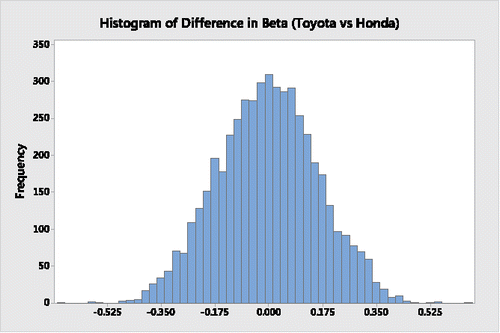
Using Minitab, the histogram in Figure 1 depicts the bootstrap distribution of differences in Sharpe ratios between Toyota and Honda, the histogram in Figure 2 displays the bootstrap distribution of the respective differences in their beta coefficients, the histogram in Figure 3 represents the bootstrap distribution of the respective differences in their alpha coefficients, and the histogram in Figure 4 provides the bootstrap distribution of the respective differences in their Treynor ratios.

Figure 1. Bootstrap distribution of the difference in Sharpe ratios for Toyota and Honda.

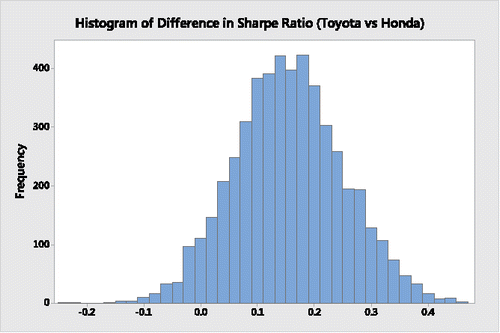
Figure 2. Bootstrap distribution of the difference in beta coefficients for Toyota and Honda.

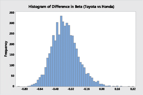
Figure 3. Bootstrap distribution of the difference in alpha coefficients for Toyota and Honda.

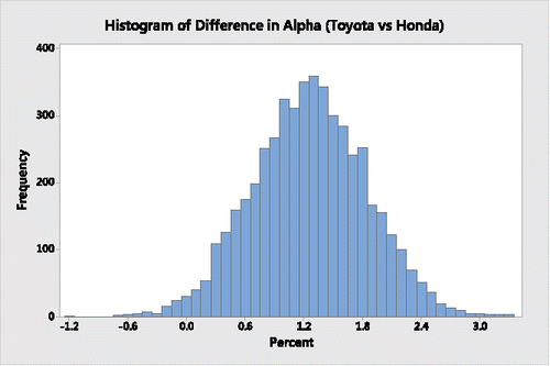
Figure 4. Bootstrap distribution of the difference in Treynor ratios for Toyota and Honda.

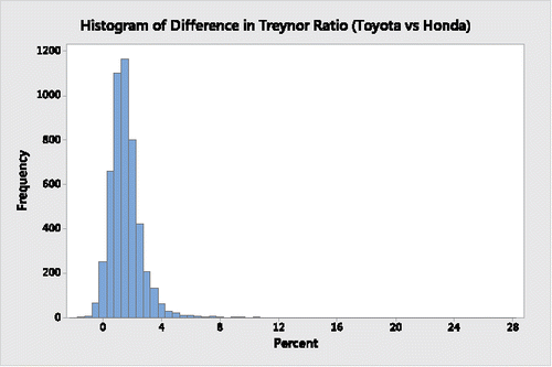
It is clear from a descriptive assessment of the results from Table 2 and Figures 1 through 4 that during the 63-month period Toyota's Sharpe ratio, beta coefficient and alpha coefficient appear to be superior to Honda's. Moreover, on average, the Toyota Treynor ratio is also superior to the Honda Treynor ratio; its greater variability is limited to the upper tail, indicating that there are many possible “high-end” outliers where Toyota's Treynor ratio is substantially higher than Honda's Treynor ratio.

5.2. Inferential Analysis via Bootstrapping

Table 3 displays the 95% bootstrap percentile confidence intervals for each measure for both companies. Any value outside a particular confidence interval is considered as performing significantly differently from the overall resampling estimate, its p-value would be below 0.05. Such tests are based on a null hypothesis with parameter equal to the estimated mean from the particular bootstrap distribution as shown in Table 2. Note that, for both Honda and Toyota, all four actually observed financial investment measures displayed in Table 2 lie within their respective “traditional 95%” confidence interval estimates of their potentially true values, demonstrating that current performance does not differ from what is expected for these companies.

Table 3. A comparison of two companies: 95% bootstrap percentile confidence interval estimates on four financial investment measures.

Measure	Sharpe	Ratio	Beta	Coef.	Alpha	Coef.	Treynor	Ratio
Confidence interval	Lower limit	Upper limit	Lower limit	Upper limit	Lower limit (%)	Upper limit (%)	Lower limit (%)	Upper limit (%)
Toyota	−0.0764	0.4353	0.2941	0.9510	−0.8528	1.7334	−0.6871	5.3532
Honda	−0.2329	0.2773	0.6313	1.3712	−2.2502	0.6392	−1.5775	2.0267
Difference	−0.0259	0.3469	−0.6276	−0.0879	0.1358	2.3973	−0.1081	4.1513

On the other hand, as shown in Table 3 and in the histograms of Figures 2 and 3, when assessing the differences in the two companies' beta and alpha coefficients the respective “traditional 95%” bootstrap percentile confidence interval estimates have lower and upper boundaries that do not contain a 0 difference, indicating from a significance-testing perspective that Toyota's beta and alpha coefficients are significantly better than Honda's.

Nevertheless, from Table 3 and from the histograms of Figures 1 and 4, when assessing the differences in the two companies' Sharpe ratios and Treynor ratios the respective “traditional 95%” bootstrap percentile confidence interval estimates do have lower and upper boundaries that contain a 0 difference. Although “traditionalists” will say that there is insufficient information to state that Toyota's Sharpe and Treynor ratios are significantly better, the proximities of the lower boundaries of both confidence intervals to 0 suggest that they actually are better.

Consider, for example, the two sets of 5000 bootstrap resamples comparing the Sharpe and Treynor ratios for Toyota versus Honda. If these had been the outcomes of contests between two teams, each of the 5000 events (i.e., bootstrap resamples) will result in a “winner” and “loser” but it is not necessary for this purpose to specify the magnitude of the difference between the competitors. With respect to the Sharpe ratios, the 5000 differences between Toyota and Honda results in 4750 “victories” for Toyota and only 250 “victories” for Honda. That is, Honda only outperformed Toyota 5.0% of the time. Moreover, with respect to the Treynor ratios, there are 4826 “victories” by Toyota and only 174 by Honda. Using this financial investment measure, Honda only outperformed Toyota 3.48% of the time. “Traditionalists” employing the usual 95% confidence interval estimates or corresponding two-sided significance tests with p-value of 0.05 would forgo the opportunity of drawing such conclusions and perhaps making more informed investment decisions.

Wasserstein and Lazar (2016) recently published the American Statistical Association's position on the concept of p-value, stating that:

Scientific conclusions and business or policy decisions should not be based only on whether a p-value passes a specific threshold. Practices that reduce data analysis or scientific inference to mechanical “bright-line” rules (such as “p < 0.05”) for justifying scientific claims or conclusions can lead to erroneous beliefs and poor decision-making. … The widespread use of “statistical significance” (generally interpreted as “p < 0.05”) making a claim of a scientific finding (or implied truth) leads to considerable distortion of the scientific process.

And further that:

Good statistical practice, as an essential component of good scientific practice, emphasizes principles of good study design and conduct, a variety of numerical and graphical summaries of data, understanding of the phenomenon under study, interpretation of results in context, complete reporting and proper logical and quantitative understanding of what data summaries mean. No single index should substitute for scientific reasoning.

5.3. Inferential Analysis via Permutation Testing

In addition to bootstrap estimation procedures for all four financial investment measures, permutation tests can be used to assess the significance of the beta coefficient for each company individually as well as to assess the difference in beta coefficients between the two companies. Permutation tests are very general and make very few distributional assumptions.

Key results are summarized in Table 4. Figure 5 is a histogram displaying the permutation distribution of the difference in beta coefficients for Toyota and Honda.

Table 4. A comparison of beta coefficients for two companies: Permutation distributions and 95% confidence interval estimates.

Company	Mean	SD	Lower limit	Upper limit
Toyota	−0.00068	0.19422	−0.38542	0.37385
Honda	0.00258	0.22714	−0.45183	0.45588
Difference	−0.00327	0.16360	−0.31881	0.31702

Figure 5. Permutation distribution of the difference in beta coefficients for Toyota and Honda.

The null hypotheses for the three respective tests are that the true slope ${\beta }_1$ for each company is 0 and that the test for the differences in the beta coefficients is 0.

Evaluating performance individually by company, based on permutation distributions comprised of 5000 permutation resamples, the actual beta coefficient for Toyota, 0.61968, shown in Table 2, has a p-value of 0.0010 and this actual beta coefficient exceeds all but 5 of the 5000 absolute permutation resampled values. In addition, the actual beta coefficient for Honda, 1.00470, shown in Table 2, has a p-value of less than 0.0001, which surpasses the absolute extreme permutation resampled value. Therefore, we can declare that the true slope or beta coefficient for each company is statistically significant. The actual beta coefficient for Honda, however, is more extreme when compared to its permutation distribution. Nevertheless, each firm's stock prices change significantly from the overall market, and the results indicate Toyota significantly outperforms Honda. This is confirmed by the permutation distribution of the difference in beta coefficients between Toyota and Honda described by the histogram in Figure 5. The actual difference in beta coefficients, −0.38502, shown in Table 2, had a p-value of 0.0132 and this difference in beta coefficients exceeded all but 66 of the 5000 absolute permutation resampled values.

Using a confidence interval approach for these hypotheses tests results in the same conclusions. The 2.5th and 97.5th percentile points of Toyota's permutation distribution for the beta coefficient are, respectively, −0.38542 to +0.37385 (far below the actual $b_1$ of +0.61968). Moreover, the 2.5th and 97.5th percentile points of Honda's permutation distribution for the beta coefficient are, respectively, −0.45183 to +0.45588 (far below the actual $b_1$ of +1.00470). Finally, the 2.5th and 97.5th percentile points of the permutation distribution for the difference in the beta coefficient for Toyota and Honda are, respectively, −0.31881 to +0.31702 (above the actual difference in the two beta coefficients −0.38502).

It is important to note that a permutation test for the difference in two beta coefficients is clearly appropriate but, despite their versatility, permutation tests cannot be devised for all statistics (Hesterberg et al. 2003). Permutation resamples must be obtained only when they are consistent with the study design and the null hypothesis and this would be impossible for testing for differences in Sharpe ratios where appropriate study design would yield a set of constant results for each permutation.

Although a permutation test for the difference in Treynor ratios may be possible, the results would be a function of the reciprocals of the beta coefficients so no new information would be gleaned. Similarly, the alpha coefficients are also based on the regression results. In both these situations, as shown in Section 5.2, bootstrap confidence intervals may be formed and the null hypotheses can be tested by determining whether the actual observed differences in the particular test statistics are captured by their corresponding confidence intervals.

5.4. Making the Investment Decision–A Caveat

It is important for students to realize that a rational decision maker must make use of data available at a particular moment in time in the decision making process. In summation, if a potential investor interested in purchasing shares of stock from either Toyota or Honda had collected the time-series datasets over the period March 2010 through May 2015 and then compared the two companies using the four aforementioned financial investment measures, by the first week in June 2015 this person would have ample evidence of the superior historical performance of Toyota over Honda. The former had most certainly outperformed the latter. Nevertheless, such a decision would be based on evidence from data available only during that specific period. A subsequent event that impacts one of the companies after May 2015 could quickly make the early June 2015 investment decision erroneous or moot.

6. Recommendations for Course Development

This article has important implications for teaching introductory business statistics at the undergraduate level. Hopefully, our suggestions will result in a useful curricular upgrade in the traditional introductory business statistics course. We also wish that these financial investment measures will be included in application sections of future editions of traditional business statistics textbooks or in new texts dedicated to the teaching of basic business statistics methods with applications in finance.

Below, we suggest topics to cover in a revised traditional course for all business students or in a dedicated course for students specifically interested in finance. For either course, we recommend introducing descriptive regression modeling (i.e., constructing the scatterplot, obtaining the sample linear regression equation, and assessing such descriptive measures as the coefficient of determination, the coefficient of correlation, and the standard error of the estimate) immediately after discussing numerical descriptive measures even though most texts separate these topics by several chapters.

6.1. A Traditional Introductory Business Statistics Course Enhanced With Financial Investment Measure Applications

The undergraduate level introductory business statistics course is normally a prerequisite to all core-required courses in the functional-area disciplines of accounting, finance, management, and marketing, and the statistics course is designed to meet the needs of those core-required courses. To achieve this, curricular flexibility and topic selection are often severely hampered.

Given that students enrolling in a traditional introductory business statistics course have varied backgrounds and interests, where some are more mathematically oriented than others, it is useful to begin with a review of fundamental mathematics needed for business (i.e., proportions, percentages, percentage change, rates, ratios, indices, and probabilities) so that the students “start at the same base.” A general overview of business statistics is then followed by data visualization through tabular and chart presentation of applications across the functional area disciplines. The next subjects to cover are numerical descriptive measures, including the Sharpe ratio with a real data application in finance. Data analysis is enhanced through the use of appropriate statistical software. The course would then contain a short chapter involving only a descriptive statistics approach to simple linear regression modeling with specific financial applications to include both the beta coefficient and alpha coefficient as measures of a company's financial performance relative to the overall stock market. (The CAPM which is described by the regression equation should, at best, be mentioned without discussion because the development of CAPM is in the purview of the core finance course). Then, it is possible to cover the Treynor ratio, which requires estimation of the beta coefficient.

Owing to the more traditional nature of the typical introductory business statistics course where presentation of the normal distribution then leads to discussions of sampling distributions, followed by classical confidence interval estimation and hypothesis testing methods applied to problems across the functional areas of business, inferential methods based on resampling (i.e., bootstrapping estimation and permutation tests) are rarely included in either the curricula or in the currently used textbooks. Nevertheless, if faculty are aware of the many virtues of resampling methods, it would be worthwhile to enhance the classroom experience by providing, at least, a brief description and demonstration of their utility.

In addition, such traditional courses should still take more appropriate advantage of the GAISE College Report recommendations pertaining to real data applications and proactively include the four financial investment measures, engaging all business students in an understanding of their utility and importance as tools in investment since it must be assumed that most students majoring in business, regardless of discipline, will probably make stock market investments in their lifetimes. Hence, coverage of the financial measures can be accomplished through active learning. Students, individually or in teams, should be assigned specific companies to investigate. They must then discuss and describe their findings and interact with classmates to learn about other companies' performance. There should be ample opportunity to accomplish this with students honing their written and oral communication skills and/or teamwork skills.

Exhibit 2 displays a written project assignment for the traditional business statistics course. A shortened variation of this has been successfully used in the core-required introductory finance course. Given that resampling methods are unlikely to be covered in either course, this project results in a thorough descriptive analysis and each student will be expected to make a 3-min oral presentation highlighting company comparisons and recommendations

Exhibit 2.

Project assignment for a traditional business statistics course.

1.	Go online and examine the list of stocks comprising the S&P 500. Select any two companies that you wish to study.
2.	Go online and collect the end-of-month closing stock prices for each of these companies for the past five years. Enter these two time series in a worksheet.
3.	Go online and collect the corresponding end-of-month closing S&P 500 index values and enter this time-series in the same worksheet.
4.	Go online to collect information about the two companies you selected to study and then write a brief introduction describing these companies.
5.	Develop separate time-series plots over the 60 months for each of these three time series.
6.	In your own words describe any differences in trends or patterns.
7.	Develop separate histograms and boxplots for each company and for the S&P 500.
8.	Obtain appropriate descriptive measures of central tendency, variation, and shape for each company's monthly closing prices and for the S&P 500 monthly index values.
9.	Prepare a brief descriptive analysis pertaining to the monthly closing prices of each company and the S&P 500 index values over the observed 60-month period.
10.	In your worksheet compute the percentage changes in monthly closing prices for each company and compute the percentage changes for the corresponding monthly closing S&P 500 index values.
11.	On the same chart, develop the time-series plots for the 59 monthly percentage changes in prices for the two companies as well as for the 59 monthly percentage changes in the S&P 500 index values.
12.	In your own words describe any differences in trends or patterns.
13.	Develop separate histograms and boxplots of monthly percentage changes for each company and for the S&P 500.
14.	Obtain appropriate descriptive measures of central tendency, variation, and shape for each company and for the S&P 500.
15.	Prepare a brief descriptive analysis pertaining to the monthly percentage changes of each company and the S&P 500 over these observed 59-month time series.
16.	Using a savings account with monthly interest rate of 0.0875% as a “risk-free” investment, compute the Sharpe ratios for each company over the 59-month series of percentage changes observed and compare your findings. Be sure to explain which company had the preferred Sharpe ratio over the observed time period.
17.	For each company develop a simple linear regression model to predict monthly percentage change in a stock's price as a function of the monthly percentage change in the S&P 500. Be sure to show the two scatterplots and the two regression equations.
18.	From each regression model, compare the beta coefficients and compare the alpha coefficients. Be sure to explain what the results mean and which company had the preferred beta and preferred alpha coefficients.
19.	Using a savings account with monthly interest rate of 0.0875% as a “risk-free” investment, compute the Treynor ratios for each company over the 59-month series of percentage changes observed and compare your findings. Be sure to explain which company had the higher Treynor ratio over the observed time period.
20.	Based on your responses to 16, 18, and 19, if you had the opportunity to purchase shares of stock in one of these companies today, which of the two companies, if either, would you prefer to invest in? Why?

Note: Your submitted written report should include a Title Page, an Introduction section (see 4), a Descriptive Study section (see 5–16), a Regression Study section (see 17–19), and a Summary and Recommendations section (see 20). The worksheets appear in the Appendix.

6.2. An Introductory Business Statistics Course Dedicated to Finance Majors

A dedicated course would begin with a review of fundamental mathematics for finance majors (i.e., proportions, percentages, percentage change, rates, ratios, indices, probabilities, odds, and logarithms) and then present data visualization through tables and charts specific to financial applications, followed by coverage of numerical descriptive measures important in finance, including the Sharpe ratio. Data analysis can be enhanced through the use of appropriate statistical software. The course would then contain a short chapter involving only a descriptive statistics approach to simple linear regression modeling with specific financial applications to include both the beta coefficient and alpha coefficient as measures of a company's financial performance relative to the overall stock market. (As previously stated, the CAPM which is described by the regression equation should, at best, be mentioned without discussion because the development of CAPM is in the purview of the core finance course.) The Treynor ratio, a measure often competing with the Sharpe ratio and dependent on the beta coefficient, would be covered next. An introductory chapter on index numbers would follow, with particular emphasis on the CPI-U (Consumer Price Index for All Urban Consumers)—its purpose, its development, its use as a price deflator, and its impact on labor-negotiated cost-of-living adjustments (COLAs) to salaries and wages. The course might also contain a chapter on an introduction to decision making and focus on applications in finance pertaining to investing or not investing.

To present the topic of statistical inference in the suggested dedicated course, it would be natural for resampling methods to replace classical methods. There is no need to teach probability distributions in such a course or to teach sampling distributions as a lead-in to classical methods of confidence interval estimation and hypothesis testing. On the other hand, teaching bootstrap percentile confidence interval estimation for the four financial investment measures described—the Sharpe and Treynor ratios, and the beta and alpha coefficients—and introducing the concepts of permutation testing that can be employed in a regression analysis (or in a correlation analysis) would be particularly appropriate. When dealing with a specific financial investment measure for a selected company, there is only one value, not a sample of values, so a method has to be chosen whereby, through simulation, a bootstrap distribution or permutation distribution could evolve to represent many “potential” resamples when only one sample is available. Such revised course curricula and textbooks aimed to serve them must reflect the important advantages that resampling methods enjoy over classical methods of inference—they are conceptually easier to teach, they make fewer, less stringent assumptions, and, when comparable, they typically yield as good or even better results (Hesterberg et al. 2003).

We envision that such a dedicated course could prominently foster active learning, where students working individually or on teams would be comparing performance of the chosen companies. Statistical software is essential for assisting in the needed data analysis and students would have the opportunity to improve oral, written, and teamwork skills through group project reports and presentations.

Exhibit 3 presents a suggested written project assignment for a business statistics course dedicated to finance majors where resampling methods are a major component of the course. A variation of this assignment has been successfully used as a term project in a corporate finance course for finance majors that also requires a 20-min oral presentation. In the business statistics course, however, each student is expected to make a 10-min oral presentation comparing their companies and to make recommendations.

Exhibit 3.

Project assignment for a business statistics course dedicated to finance majors.

1.	Go online and examine the list of stocks comprising the S&P 500. Select any two companies that you wish to study.
2.	Go online and collect the end-of-month closing stock prices for each of these companies for the past five years. Enter these two time series in a worksheet.
3.	Go online and collect the corresponding end-of-month closing S&P 500 index values and enter this time series in the same worksheet.
4.	Go online to collect basic information on the two companies you selected to study, including key accounting and financial investment measures, and then write a brief introduction describing these companies.
5.	In your worksheet compute the percentage changes in monthly closing prices for each company and compute the percentage changes for the corresponding monthly closing S&P 500 index values.

Descriptive Analysis:

6.	Based on 5, obtain appropriate descriptive measures of central tendency, variation, and shape for each company and for the S&P 500.
7.	Prepare a brief descriptive analysis pertaining to the monthly percentage changes of each company and the S&P 500 over these observed 59-month time series.
8.	Using a savings account with monthly interest rate of 0.0875% as a “risk-free” investment, compute the Sharpe ratios for each company over the 59-month series of percentage changes observed and compare your findings. Be sure to explain which company had the preferred Sharpe ratio over the observed time period.
9.	For each company develop a simple linear regression model to predict monthly percentage change in a stock's price as a function of the monthly percentage change in the S&P 500. Be sure to show the two scatterplots and the two regression equations.
10.	From each regression model, compare the beta coefficients and compare the alpha coefficients. Be sure to explain what the results mean and be sure to explain which company had the preferred beta and alpha coefficients.
11.	Using a savings account with monthly interest rate of 0.0875% as a “risk-free” investment, compute the Treynor ratios for each company over the 59-month series of percentage changes observed and compare your findings. Be sure to explain which company had the higher Treynor ratio over the observed time period.
12.	From your responses to 8, 10, and 11, if you had the opportunity to purchase shares of stock in one of these companies today, which of the two companies, if either, would you prefer to invest in? Why?

Inferential Analysis:

13.	Using the 59 monthly percentage changes in prices for each company and corresponding results from 8, use the same random seed to develop the two bootstrap distributions each having 5000 Sharpe ratios and construct their histograms.
14.	Form the resampling distribution of the differences in corresponding 5000 Sharpe ratios and construct its histogram. Sort the results and develop the 95% bootstrap percentile confidence interval estimate of the difference in the Sharpe ratios. What can you conclude?
15.	As per 9, for each company use the pairs of 59 monthly company price and S&P 500 index value percentage changes. Then, starting with the same random seed as in 13, develop the two bootstrap distributions each having 5000 beta coefficients and construct their histograms.
16.	Form the resampling distribution of the differences in corresponding 5000 beta coefficients and construct its histogram. Sort the results and develop the 95% bootstrap percentile confidence interval estimate of the difference in the beta coefficients. What can you conclude?
17.	As per 9, for each company use the pairs of 59 monthly company price and S&P 500 index value percentage changes. Then, starting with the same random seed as in 13, develop the two bootstrap distributions each having 5000 alpha coefficients and construct their histograms.
18.	Form the resampling distribution of the differences in corresponding 5000 alpha coefficients and construct its histogram. Sort the results and develop the 95% bootstrap percentile confidence interval estimate of the difference in the alpha coefficients. What can you conclude?
19.	Using the 59 monthly percentage changes in prices for each company and corresponding results from 11 and 15, use the same random seed to develop the two bootstrap distributions each having 5000 Treynor ratios and construct their histograms.
20.	Form the resampling distribution of the differences in corresponding 5000 Treynor ratios and construct its histogram. Sort the results and develop the 95% bootstrap percentile confidence interval estimate of the difference in the Treynor ratios. What can you conclude?
21.	Based on the four bootstrap distributions of differences in the financial investment measures in 14, 16, 18, and 20 analyze the results and be sure to state which company you believe has performed better over the 59-month period.
22.	As per 9, for each company use the pairs of 59 monthly company price and S&P 500 index value percentage changes and, starting with the same random seed as in 13 develop the two permutation distributions each having 5000 beta coefficients. Construct their histograms.
23.	Form the resampling distribution of the differences in corresponding 5000 beta coefficients and construct its histogram. Sort the results and develop the 95% permutation percentile confidence interval estimate of the difference in the beta coefficients. Is 0 contained in the interval? What can you conclude?
24.	As per 22, for each company sort the results and develop the 95% permutation percentile confidence interval estimate of the beta coefficient. For each company determine whether the actual beta coefficient obtained in 10 is contained in the respective intervals. What do your results indicate?
25.	As per 8 and 14, determine whether the actual difference in the two company Sharpe ratios is contained in the 95% bootstrap percentile confidence interval estimate of the difference in the Sharpe ratios. What do your results indicate?
26.	As per 10 and 18, determine whether the actual difference in the two company alpha coefficients is contained in the 95% bootstrap percentile confidence interval estimate of the difference in the alpha coefficients. What do your results indicate?
27.	As per 11 and 20, determine whether the actual difference in the two company Treynor ratios is contained in the 95% bootstrap percentile confidence interval estimate of the difference in the Treynor ratios. What do your results indicate?
28.	Based on the tests in 23–27 analyze your findings and be sure to state which company you believe has performed better over the 59-month period.
29.	Compare your answers in 21 and 28 and comment on the consistency of conclusions you had drawn. Next, compare this to your answers in 12 and comment on the consistency of conclusions you had drawn.
30.	In summation, based on your responses to 29, if you had the opportunity to purchase shares of stock in one of these companies today, which of the two companies, if either, would you prefer to invest in? Why?

Note: Your submitted written report should include a Title Page, an Introduction section (see 4), a Descriptive Analysis section (6–12), an Inferential Analysis Using Bootstrapping section (13–21), an Inferential Analysis Using Permutation Testing section (22–24), an Inferential Analysis Using Bootstrap Confidence Intervals to Approximate Permutation Testing section (25–28), and a Summary and Recommendations section (30). The worksheets appear in the Appendix.

6.3. Traditional versus Dedicated Course: A Reflection

Given that the traditional business statistics course that has been taught for five decades is general in format and provides applications to all the functional disciplines, it is important to address why a dedicated course is appropriate, particularly when the current move in business schools on many campuses is to break down silos and show business as an integrated theme with all the component disciplines resulting in a holistic view of how a company operates. We contend here, however, that one can enthusiastically support the idea that breaking down silos in teaching the business core is an effective approach and also believe that teaching statistics, which is prerequisite to that core may be best served in silos. The key driver reflecting dedicated course pedagogy is motivation, and this impacts on both the students enrolling in the course and the faculty teaching it.

Presumably, such a course dedicated to intended finance majors will be of more interest to the student participants and, at the same time, enable the students to personally assess whether finance is the field they wish to pursue. Students fearful or anxious about taking a course in statistics might feel less so if the topics covered and applications presented were aligned to their interests. Moreover, faculty with discipline-specific knowledge may be more enthusiastic about having the opportunity to teach fundamental statistics within their own specialty, using topics and applications to which they can best relate.

Based on an evaluation of the strengths and weaknesses of these two suggested course revisions, we contend that both will clearly enhance current traditional offerings for introductory business statistics students and that authors of traditional texts should carefully consider our recommendations. Moreover, we believe that a course dedicated specifically to finance majors would best serve the needs of its students. This will require curricular revision that includes the introduction and coverage of resampling methods and leads to the development of new textbooks for such a dedicated course.

Whether it is driven “top-down” or “bottom up,” curriculum change is almost always a slow process owing to constraints in budgets, concerns for accreditation, departmental competition, faculty inertia, and/or conviction. As a start, experimentation through special sections of multi-section core-required courses enables self-assessment and student feedback that leads to course refinement and, eventually, curriculum change. At our institution, we are planning the experimental implementation for the upcoming semester in a traditional course section with the expectation that a freshmen-learning-community based on interests in finance will provide the student body for a dedicated course section in the following semester. The aforementioned projects described in Exhibits 2 and 3 will be put to the test in these introductory-level courses.

Supplementary Material

The Appendices appear in the online supplementary information, which can be accessed on the publisher's website.

Acknowledgments

The development of this article was supported in part through the Khubani/TelebrandsFaculty Research Fellowship awarded to Mark L. Berenson in the Feliciano School of Business at Montclair State University.

References

- Aliaga, M., Cobb, G., Cuff, C., Garfield, J. (Chair), Gould, R., Lock, R., Moore, T., Rossman, A., Stephenson, B., Utts, J., Velleman, P., and Witmer, J. (2005), GAISE (Guidelines for Assessment and Instruction in Statistics Education) College Report, Alexandria, VA: American Statistical Association.
- Bernstein, P.L. (1992), Capital Ideas: The Improbable Origins of Modern Wall Street, New York: Free Press.
- Carver, R., Everson, M. (Co-chair), Gabrosek, J., Holmes Rowell, G., Horton, N., Lock, R., Mocko, M. (Co-chair), Rossman, A., Velleman, P., Witmer, J., and Wood, B. (2016), Guidelines for Assessment and Instruction in Statistics Education (GAISE) College (DRAFT) Report, Alexandria, VA: American Statistical Association.
- Chang, G. E., Kerns, G. J., Lee, D. J., and Stanek, G. L. (2009), “Calibration Experiments for a Computer Vision Oyster Volume Estimation System,” Journal of Statistics Education, 17.
- Coakley, C. W. (1996), “Suggestions for Your Nonparametric Statistics Course,” Journal of Statistics in Education, 4.
- Cobb, G. (2007), “The Introductory Statistics Course: A Ptolemaic Curriculum?,” Technology Innovations in Statistics Education, 1, 16. Available at http://repositories.cdlib.org/uclastat/cts/tise/vol1/iss1/art1/.
- ——— (2013), “What Might a Twenty-Year Old Conference Tell Us About the Future of Our Profession?,” Journal of Statistics Education, 21, 17.
- del Mas, R. C., Garfield, J., and Chance, B. L. (1999), “A Model of Classroom Research in Action: Developing Simulation Activities to Improve Students' Statistical Reasoning,” Journal of Statistics in Education, 7.
- eCOTS16: Electronic Conference on the Teaching of Statistics (2016), Penn State University. Available at https://www.causeweb.org/cause/ecots/ecots16.
- Ernst, M. D. (2004), “Permutation Methods: A Basis for Exact Inference,” Statistical Science, 19, 676–685.
- ——— (2009), “Teaching Inference for Randomized Experiments,” Journal of Statistics Education, 17.
- Eudey, T. L., Kerr, J. D., and Trumbo, B. E. (2010), “Using R to Simulate Permutation Distributions for Some Elementary Experimental Designs,” Journal of Statistics Education, 18, 30.
- Everson, M., and Mocko, M. (2015a), Updating the Guidelines for Assessment and Instruction in Statistics Education (GAISE). Available at www.causeweb.org/webinar/teaching/2015-07/index.php.
- ——— (2015b), “GAISE into the Future: Updating a Landmark Report for an Increasingly Data-Centric World,” in annual Joint Statistics Meetings (JSM), Seattle, WA.
- Forbes, S. (2014), “Using Action Research to Develop a Course in Statistical Inference for Workplace-Based Adults,” Journal of Statistics Education, 22.
- Garrett, L., and Nash, J. C. (2001), “Issues in Teaching the Comparison of Variability to Non-Statistics Students,” Journal of Statistics Education, 9.
- Graham, J., and Harvey, C. (2002), “How Do CFOs Make Capital Budgeting and Capital structure Decisions,” Journal of Applied Corporate Finance, 15, 8–23.
- Hesterberg, T., Monaghan, S., Moore, D. S., Clipson, A., and Epstein, R. (2003), “Bootstrap Methods and Permutation Tests,” Companion Chapter 18 in The Practice of Business Statistics, eds. Moore, D. S., McCabe, G. P., Duckworth, W. M., and Sclove, S. L., New York: W. H. Freeman and Company.
- Jaggia, S., and Kelly, A. (2013), Business Statistics: Communicating with Numbers. New York: McGraw-Hill.
- Jensen, M. C. (1968), “The Performance of Mutual Funds in the Period 1945–1964,” Journal of Finance, 23, 587–636.
- Jordan, B., and Miller, T. (2012), Fundamentals of Investments: Valuation and Management (6th ed.), New York: McGraw-Hill.
- Linter, J. (1965), “The Valuation of Risk Assets and the Selection of Risky Investments in Stock Portfolios and Capital Budgets,” Review of Economics and Statistics, 47, 13–37.
- Lock, R. (2004), “Proposed Guidelines for Teaching Statistics: K-12 and College,” Panel discussion at annual Joint Statistical Meetings (JSM), Toronto, Canada.
- Lock, R., Lock, P., Lock Morgan, K., Lock, E., and Lock, E. (2013), Statistics: Unlocking the Power of Data, New York: Wiley.
- Markowitz, H. M. (1952), “Portfolio Selection,” Journal of Finance, 7, 77–91.
- ——— (1959), Portfolio Selection: Efficient Diversification of Investments, New York: Wiley.
- Mondello, J. (Nov, 2015), AACSB DataDirect ≤[email protected]≥
- Mossin, J. (1966), “Equilibrium in a Capital Asset Market,” Econometrica, 34, 768–783.
- Ross, S. A., Westerfield, R. W., and Jordan, B.D. (2016), Fundamental of Corporate Finance (11th ed.), New York: McGraw Hill Education.
- Rossman, A., and Chance, B. (2008), Concepts of Statistical Inference: A Randomization-Based Curriculum. Available at http://statweb.calpoly.edu/csi.
- Rossman, A., and Chance, B. (2012), Workshop Statistics: Discovery with Data, (4th ed.), New York: Wiley.
- Rossman, A., and Cobb, G. (2015), “Interview with George Cobb,” Journal of Statistics Education, 23, 29.
- Sharpe, W. F. (1964), “Capital Asset Prices: A Theory of Market Equilibrium,” Journal of Finance, 14, 425–442.
- ——— (1966), “Mutual Fund Performance,” Journal of Business, 39, 119–138.
- Simon, J. L. (1994), “What Some Puzzling Problems Teach About the Theory of Simulation and the Use of Resampling,” The American Statistician, 48, 290–293.
- Simon, J. L., and Bruce, P. (1991), “Resampling: A Tool for Everyday Statistical Work,” Chance: New Directions for Statistics and Computing, 4, 22–32.
- Stephenson, W. R., Froelich, A. G., and Duckworth, W. M. (2010), “Using Resampling to Compare Two Proportions,” Teaching Statistics, 32, 66–71.
- Stine, R., and Foster, D. (2011), Statistics for Business: Decision Making and Analysis, Boston, MA: Addison-Wesley.
- The Charles Schwab Corporation. (2015), “Getting Smart on Beta,” available at https://www.schwab.com/resource-center/insights/content/getting-smart-on-beta.
- Tintle, N., VanderStoep, J., Holmes, V., Quisenberry, B., and Swanson, T. (2011), “Development and Assessment of a Preliminary Randomization-Based Introductory Statistics Curriculum,” Journal of Statistics Education, 19, 25.
- Tintle, N., Chance, B., Cobb, G., Rossman, A., Roy, S., Swanson, T., and Vanderstoep, J. (2015), Introduction to Statistical Investigations, New York: Wiley.
- Treynor, J. L. (1966), “How to Rate Management Investment Funds,” Harvard Business Review, 43, 63–75.
- Wasserstein, R. L., and Lazar, N. A. (2016), “The ASA's Statement on p-Values: Context, Process and Purpose,” The American Statistician, 70, 129–133.
- Wood, M. (2005), “The Role of Simulation Approaches in Statistics,” Journal of Statistics in Education, 13.