Punching a Ticket to Cooperstown

ABSTRACT

When exposed to principal components analysis for the first time, students can sometimes miss the primary purpose of the analysis. Often the focus is solely on data reduction and what to do after the dimensions of the data have been reduced is ignored. The datasets discussed here can be used as an in-class example, a homework assignment, or a written project, with a focus in this article as an in-class example. The data give the students an opportunity to perform principal components analysis and follow-up analyses on a real dataset that is not necessarily the easiest to handle.

KEYWORDS:

• Baseball
• Classification
• Logistic regression
• Principal components analysis

1 Introduction

Cooperstown, a small village in upstate New York, has been synonymous with baseball immortality ever since the founding of the National Baseball Hall of Fame and Museum there in 1939. From the stands at the ballpark, to barstools, dorm rooms, and internet chatrooms, baseball fans have long debated what players should and should not be in Major League Baseball’s Hall of Fame.

The rules for being elected to the Hall of Fame have changed quite a bit since the first class of Ty Cobb, Walter Johnson, Christy Mathewson, Babe Ruth, and Honus Wagner was elected in 1936. In its current format adopted in 2014, the Baseball Writer’s Association of America (BBWAA) consider any player for potential election to the Hall of Fame after that player has been retired for five years. Baseball writers eligible to vote can vote for up to 10 candidates on a single ballot. Any candidate receiving votes on at least 75% of the ballots is elected to the Hall of Fame. If the player fails to reach the 75% threshold, they will be on the ballot the next year assuming that they received votes on at least 5% of the ballots cast, otherwise they can no longer appear on the ballot the following year. Players can be on the ballot for up to 10 years. Players that are not elected to the Hall of Fame in this manner are then moved to an Eras Committee system where they can be evaluated and potentially elected into the Hall of Fame at any time (Baseball Hall of Fame 2018a). These Eras Committees are commonly referred to as the “Veterans Committee”; however, they are committees made up of former managers, umpires, executives, and retired players from the following time periods (Baseball Hall of Fame 2018b):

• Today’s Game—1988 to present

• Modern Baseball—1970 to 1987

• Golden Days—1950 to 1969

• Early Baseball—1871 to 1949.

Since players in this dataset have careers that span from Major League Baseball’s early days to the present, it is important to note how players were elected to the Hall of Fame prior to 2014. The election cycles have not always been consistent. From 1936 to 1939, the elections were held annually with no real set rules in place. From 1940 to 1945, the elections were held every three years, meaning they were held in 1942 and 1945 only. This may be due to baseball players serving in World War II. From 1946 to 1956, elections were once again an annual event. From 1957 to 1965, the elections were held every other year. Since 1966, elections have been an annual occurrence. Typically there are no run-off ballots; however, in 1946 the top 20 vote getters comprised a second and final ballot, if no one was elected, and no one was in 1946’s election. In 1949, there was a run-off vote, with Detroit Tigers’ second baseman Charlie Gehringer being elected to the Hall of Fame. From 1960 to 1968, there were run-off ballots where the top 30 vote getters comprised a second and final ballot, if no one was elected. In 1968, there was a limit implemented of 40 players per ballot. In 1945, voters were supposed to focus more on how the game was played on the field instead of a player’s character off the field. In terms of waiting periods for players retired to be eligible for election, from 1936 to 1945 there was no waiting period. From 1946 to 1953, a player needed to have been retired one year. In 1954, a player needed to be retired for five years prior to being eligible for election. In 1979, the “at least appearing on 5% of ballots” rule was introduced. From 1946 to 1955, a player could not be on the ballot if they have been retired for 25 years. This period was extended to 30 years in 1956. In 1962, it was reduced to 20 years. In 2014, it was reduced to its current 15-year period (Baseball Hall of Fame 2018c).

The data described here will focus on position players, that is, nonpitchers, who have received at least one vote for the Hall of Fame at some point in their careers. The dataset will be used as an example of principal components analysis as well as using the principal components in a logistic regression model to predict the probability of a player being enshrined into the Hall of Fame. The principal components analysis will be used to reduce the dimensions of the dataset. Logistic regression will then be performed using the retained principal components as predictors to predict the probability of a hitter being inducted into the Hall of Fame.

Specifically in this manuscript, methods and results will be presented in a way for instructors to use the dataset as an in-class example; however, instructors may wish to use this dataset for a homework assignment or as part of a data analysis project. Along the way, helpful hints, potential pitfalls, and alternative applications will be introduced to provide further guidance for any instructors. It should be noted that this type of analysis would work best for upper-level undergraduate mathematics or statistics students and first-year graduate students taking an applied statistics sequence. For the record, these data were specifically used in a master’s level applied statistics sequence at an institution where the sequence has no prerequisites and students need to have taken one linear algebra course during their academic career to be accepted into the program. This type of course might use a textbook like the one by Ramsey and Schafer (2013), where the topics of principal components and logistic regression are addressed.

Helpful Hint: If using a textbook like Ramsey and Schafer’s (2013) The Statistical Sleuth, an instructor will have to supplement the material involving principal components analysis with all of the necessary linear algebra needed for students to really grasp what is going on. While a very useful textbook, Ramsey and Schafer omit all of the underlying linear algebra calculations.

2 The Data and the Story

The data in the file baseballHOF.csv consist of all 602 position players that have received at least one vote for Major League Baseball’s Hall of Fame. All of the data were compiled from baseball-reference.com (Baseball Reference 2018). The variables are summarized in Table 1. All of these variables except for JAWSratio are found on the website. These metrics, though not a complete list of what can actually be measured on position players in the game, represent a mix of “traditional” and “modern” baseball statistics. The more traditional statistics are the career counting statistics, like batting average, hits, home runs, and runs batted in. Statistics like OPS have started to gain more traction in the baseball community in recent years, even appearing in nationally televised games and on scoreboards in baseball stadiums. Statistics like WAR are considered more “modern” baseball statistics. These attempts to measure a player’s offensive and defensive contributions to their team’s success.

Table 1 Description of variables.

Variable name	Variable description
Name	Name of the player—identifies the case in the data.
HoF	A “Yes”/“No” indicator on whether or not the player is in the Hall of Fame.
Yrs	Number of seasons played in player’s career.
WAR	Baseball Reference’s measure of Wins Above Replacement.
	This is a single number that describes the number of wins the player added to their teams over the course of their career.
WAR7	The sum of the seven best seasons of WAR in the player’s career.
	It may not be seven seasons in a row.
JAWS	Developed by Baseball Prospectus. It contains a combination of career and 7-year peak WAR totals allowing for comparison to average Hall of Fame players by position.
Jpos	The average JAWS score for all Hall of Fame players at this position plus overall Hall of Fame averages for positions with fewer inducted players.
JAWSratio	JAWS divided by Jpos and multiplied by 100.
G	Games played during a player’s career.
AB	At bats during a player’s career.
R	Runs scored during a player’s career.
H	Hits during a player’s career.
HR	Home runs hit during a player’s career.
RBI	Runs batted in during a player’s career.
SB	Stolen bases during a player’s career.
BB	Walks (bases on balls) during a player’s career.
BA	Batting average. This is H divided by AB.
OBP	On base percentage. This is the sum of H, BB, and times hit by a pitch divided by the sum of AB, BB, times hit by a pitch, and sacrifice flies.
SLG	Slugging percentage. This is the number of bases divided by AB.
	Every single is one base, double is two bases, triple is three bases, and HR is four bases in the numerator of this calculation.
OPS	The sum of OBP and SLG.
OPSadj	OPS adjusted to the player’s ball park. 100 is an “average” hitter.

Helpful Hint: Obviously not all students are baseball fans. When introducing these data to the students in class or as an assignment or project, be sure to open the dataset and walk them through the various variables. Take careful consideration when discussing the variables JAWS, Jpos, and JAWSratio. More details about these three variables are in the following Potential Pitfall.

Potential Pitfall: The variables JAWS and Jpos are meant to be compared with one another. Jpos is a variable that basically attempts to keep track of the player’s position, a categorical variable, via a quantitative variable. For example, Chipper Jones, Brooks Robinson, and Mike Schmidt are three Hall of Fame third basemen in the dataset. They all have a Jpos of 55.7. JAWSratio, JAWS divided by Jpos and multiplied by 100, is calculated so that any ratio greater than 100 means that the player had a higher value of JAWS compared to all other Hall of Fame players at that given position while a ratio less than 100 means that the player had a lower value of JAWS compared to all other Hall of fame players at that given position. When incorporating this information into the model, encourage students to use JAWSratio since it captures information from JAWS and Jpos.

3 The Analysis

All analyses were conducted using R version 3.4.3 (R Core Team 2018). Table 2 contains summary statistics for the 17 quantitative variables of interest for position players in the Hall of Fame and those position players who received votes but failed to make the Hall of Fame. Table 3 is the correlation matrix for the 17 quantitative variables of interest. If one includes all of these 17 variables as predictors in a model, severe multicollinearity occurs. The results of said model can be found in Table 4. It should be noted that the variance inflation factors for a logistic regression model using all of these variables as predictors range from 2.786 for stolen bases (SB), the only one less than 5, to 3217.564 for OPS. These variance inflation factors were calculated using the car package in R (Fox and Weinberg 2011). For more details, see the code in the online appendix. Since the variables are all on different scales, principal components based off the correlation matrix is the most appropriate method here.

Table 2 Summary statistics.

Not in Hall of Fame
n = 447
	Mean	SD	Min.	Q1	Median	Q3	Max.
Yrs	14.96	3.37	4.00	13.00	15.00	17.00	24.00
WAR	30.58	17.67	–5.30	17.60	29.10	40.80	162.80
WAR7	24.12	10.35	0.00	16.75	24.40	30.95	72.20
JAWSratio	50.239	25.05	–4.55	31.24	50.35	65.19	220.19
G	1662	486.11	67	1337	1673	1996	3592
AB	5836	1872.89	186	4588	5923	7129	14053
R	824.6	325.17	25.0	617.5	832.0	1031.5	2227.0
H	1622	549.82	54	1252	1621	1992	4256
HR	145.5	127.47	1.0	39.0	105.0	231.5	762.0
RBI	776.7	344.26	24.0	513.5	728.0	1026.5	1996.0
SB	125.7	129.99	2.0	37.5	80.0	172.0	752.0
BB	600.2	306.18	7.0	382.5	559.0	792.5	2558.0
BA	0.277	0.020	0.208	0.264	0.276	0.290	0.356
OBP	0.345	0.029	0.254	0.326	0.345	0.364	0.444
SLG	0.413	0.060	0.256	0.369	0.411	0.455	0.607
OPS	0.758	0.081	0.529	0.704	0.760	0.811	1.051
OPSadj	107.1	19.85	22.0	94.0	109.0	120.0	182.0
Hall of Fame
n = 155
	Mean	SD	Min.	Q1	Median	Q3	Max.
Yrs	18	3.46	10.00	16.00	18.00	20.00	27.00
WAR	67.05	26.88	16.20	49.50	63.00	75.45	162.10
WAR7	42.25	11.59	18.90	34.65	41.30	48.00	84.70
JAWSratio	99.68	33.04	30.45	76.41	96.49	114.09	213.49
G	2162	480.99	1211	1792	2164	2499	3308
AB	8001	1796.00	4205	6623	8134	9282	12364
R	1336	325.01	579	1092	1291	1592	2295
H	2418	568.11	1161	2045	2386	2826	4189
HR	225.3	181.52	11.0	74.0	169.0	360.0	755.0
RBI	1234	386.20	530	951	1208	1526	2297
SB	227.5	223.16	8.0	68.0	153.0	333.0	1406.0
BB	916.5	391.11	308.0	644.0	848.0	1118.5	2190.0
BA	0.302	0.024	0.253	0.284	0.303	0.319	0.366
OBP	0.377	0.030	0.299	0.357	0.376	0.395	0.482
SLG	0.465	0.065	0.316	0.427	0.462	0.505	0.690
OPS	0.841	0.086	0.653	0.797	0.837	0.888	1.164
OPSadj	128.8	20.95	82.0	115.0	128.0	141.0	206.0

Table 3 Correlation matrix for the 17 quantitative variables of interest (lower triangle).

	Yrs
Yrs	1.000	WAR
WAR	0.595	1.000	WAR7	JAWS
WAR7	0.504	0.954	1.000	ratio
JAWSratio	0.580	0.984	0.968	1.000	G
G	0.847	0.733	0.679	0.712	1.000	AB
AB	0.779	0.734	0.691	0.710	0.973	1.000	R
R	0.675	0.849	0.804	0.814	0.849	0.896	1.000	H
H	0.743	0.786	0.742	0.759	0.927	0.972	0.927	1.000	HR
HR	0.409	0.567	0.579	0.574	0.558	0.512	0.541	0.478	1.000	RBI
RBI	0.651	0.773	0.750	0.764	0.792	0.796	0.811	0.818	0.807	1.000
SB	0.303	0.368	0.320	0.328	0.346	0.409	0.512	0.423	–0.126	0.117
BB	0.589	0.794	0.751	0.773	0.738	0.688	0.793	0.672	0.635	0.699
BA	0.143	0.487	0.508	0.482	0.216	0.307	0.496	0.507	0.106	0.428
OBP	0.204	0.637	0.663	0.640	0.282	0.288	0.568	0.425	0.328	0.482
SLG	0.224	0.576	0.633	0.593	0.345	0.351	0.520	0.439	0.792	0.755
OPS	0.237	0.647	0.698	0.660	0.352	0.359	0.582	0.472	0.694	0.722
OPSadj	0.273	0.704	0.744	0.713	0.367	0.371	0.588	0.480	0.624	0.692
	SB
SB	1.000	BB
BB	0.262	1.000	BA
BA	0.211	0.226	1.000	OBP
OBP	0.175	0.665	0.729	1.000	SLG
SLG	–0.095	0.499	0.579	0.655	1.000	OPS
OPS	–0.006	0.601	0.683	0.835	0.963	1.000	OPSadj
OPSadj	0.096	0.601	0.645	0.812	0.873	0.926	1.000

Table 4 Estimated coefficients for the logistic regression model: all predictors.

	Estimate	SE	z-value	p-value	VIF
Intercept	–29.521	10.324	2.859	0.004
Yrs	0.196	0.107	1.827	0.068	5.265
WAR	–0.045	0.044	–1.021	0.307	24.771
WAR7	0.092	0.053	1.732	0.083	8.949
JAWSratio	0.075	0.029	2.628	0.009	18.262
G	–0.004	0.003	–1.294	0.196	70.577
AB	0.002	0.002	1.378	0.168	305.547
R	0.002	0.002	1.157	0.247	16.338
H	–0.005	0.004	–1.148	0.251	217.261
HR	–0.003	0.004	–0.818	0.413	17.582
RBI	0.004	0.001	3.022	0.003	9.339
SB	–0.001	0.001	–0.537	0.591	2.786
BB	–0.005	0.002	–2.229	0.026	23.187
BA	30.070	37.774	0.796	0.426	24.439
OBP	124.293	115.247	1.078	0.281	391.423
SLG	60.916	112.795	0.540	0.589	2083.015
OPS	–71.714	112.334	–0.638	0.523	3217.564
OPSadj	–0.031	0.022	–1.385	0.166	6.715

Using principal components analysis can help solve the problem of multicollinearity in the model. In practice, multicollinearity does not cause any issues with the model’s ability to make predictions; however, the standard errors of the regression coefficients tend to be inflated in the presence of other highly correlated predictor variables (Neter et al. 1996). If a researcher is using a variable selection method like forward, backward, or stepwise selection based on the t-statistic, for example, potentially important predictors will be discarded from the model since their possible larger standard errors will make the predictor seem less significant than what it might actually be.

Potential Pitfall: If not given proper guidance on an assignment or project, students may just include all of the predictors into a logistic regression model and ignore any issues pertaining to multicollinearity since it generally will not impact the model’s fit or its ability to make predictions (Neter et al. 1996). While performing principal components analysis does not address multicollinearity in a linear model, it can be useful in this situation since principal components are linearly uncorrelated with one another.

The goal of principal components analysis is to transform the original variables into a system of orthogonal variables and to use as few of these transformed variables as possible to describe the variation in the original dataset. Each hitter’s offensive variables are transformed via$${\mathbf{z}}_i=\mathbf{A}{\mathbf{y}}_i^{\ast },\hspace{1em}i=1,\dots ,602,$$where ${\mathbf{z}}_i$ represents the principal component scores for the ith hitter, A is an orthogonal matrix, and ${\mathbf{y}}_i^{\ast }$ are the standardized variables for the ith hitter. The correlation matrix of the offensive variables, R, can be found in Table 3. The sample covariance matrix of z will be a diagonal matrix with $s_{z_1}^2,\dots ,s_{z_{17}}^2$ on the diagonal. This matrix will be equal to $\mathbf{AR}{\mathbf{A}}^{\mathbf{T}}$. Rencher (1995) employed a spectral decomposition argument to state that since A is an orthogonal matrix, the values $s_{z_p}^2,p=1,\dots ,17$, will be equal to the eigenvalues of R. Also, the rows of A are the normalized eigenvectors of R. The eigenvalues for the correlation matrix can be found in Table 5. These will be investigated to determine the number of principal components that will be necessary to use in this analysis.

Table 5 Eigenvalue for the correlation matrix of the quantitative variables of interest.

Component	Eigenvalue	Percent of variance	Cumulative percent
1	10.6494	62.64	62.64
2	2.6160	15.39	78.03
3	1.4537	8.55	86.58
4	0.7307	4.30	90.88
5	0.4824	2.84	93.72
6	0.4314	2.54	96.26
7	0.2936	1.73	97.98
8	0.0988	0.58	98.56
9	0.0770	0.45	99.02
10	0.0520	0.31	99.32
11	0.0473	0.28	99.60
12	0.0278	0.16	99.77
13	0.0185	0.11	99.87
14	0.0109	0.06	99.94
15	0.0079	0.05	99.99
16	0.0024	0.01	100.00
17	0.0001	0.00	100.00
	17.0000

Rencher (1995) proposed some guidelines to assist in this process. Two of the simplest for students to understand is retaining enough components so that at least 80% of the total variance is explained and ignoring components whose eigenvalues are less than one. This latter criterion is known as the Kaiser criterion or Kaiser–Guttman rule (Guttman 1954; Kaiser 1970). Basically, if the measured variables are standardized, they have a variance equal to one. The eigenvalues represent the variance of the principal component. If the eigenvalue is less than one, it fails to account for as much variability as a single measured variable. However, Preacher and MacCallum (2003) said researchers misapply this rule because they ignore the fact that it was originally supposed to be a lower bound on the number of components in principal components analysis or factors in exploratory factor analysis to retain. Since the goal of this analysis is to use principal components as predictors in a logistic regression model, the approach taken will be one similar to one taken by Milewska et al. (2014). A variable selection process, specifically a backward selection procedure using p-values from the z-tests for the estimated logistic regression coefficients for this baseball analysis, will be used to determine how many principal components will be retained in the model. Using this method, potentially significant linear combinations of the hitters’ variables will not be ignored, even if the components do not necessarily explain a large proportion of variation of the original variables. The results of this variable selection procedure can be found in Table 6. The original dataset of 17 variables has now been reduced to eight principal components.

Table 6 Results of backward selection procedure: z-statistic p-values with $\alpha =0.05$.

Principal	Iterations
component	#1	#2	#3	#4	#5	#6	#7	#8	#9	#10
z1	0.000	0.000	0.000	0.000	0.000	0.000	0.000	0.000	0.000	0.000
z2	0.624	0.635
z3	0.000	0.000	0.000	0.000	0.000	0.000	0.000	0.000	0.000	0.000
z4	0.082	0.084	0.083	0.084	0.057	0.041	0.016	0.012	0.017	0.019
z5	0.000	0.000	0.000	0.000	0.001	0.001	0.001	0.001	0.002	0.003
z6	0.000	0.000	0.000	0.000	0.000	0.000	0.000	0.000	0.000	0.000
z7	0.214	0.206	0.218	0.231	0.295
z8	0.231	0.221	0.239	0.239
z9	0.177	0.143	0.154	0.147	0.231	0.259
z10	0.140	0.139	0.144	0.158	0.113	0.097	0.062	0.094
z11	0.003	0.003	0.003	0.004	0.001	0.001	0.000	0.001	0.001	0.002
z12	0.041	0.042	0.044	0.047	0.044	0.035	0.025	0.036	0.052
z13	0.161	0.158	0.152	0.150	0.097	0.110	0.108
z14	0.042	0.042	0.040	0.045	0.031	0.018	0.009	0.005	0.007	0.012
z15	0.837
z16	0.190	0.197	0.155	0.151	0.085	0.046	0.010	0.011	0.021	0.046
z17	0.525	0.517	0.526

NOTE: A bold value represents the p-value from the z-test for the estimated logistic regression coefficient of the variable eliminated at that specific iteration of the backward selection procedure using a significance level of 0.05.

Table 7 shows the eigenvectors for the eight retained components of the quantitative variables of interest. These eigenvectors represent the coefficients for each of the eight retained principal components. Denoting the principal components as z_i, as seen previously, the principal components are$$\begin{array}{c}{z}_i={\mathbf{a}}_i^{\mathbf{T}}{\left({\mathbf{S}}^{1/2}\right)}^{-1}\left(\mathbf{y}-\overline{\mathbf{y}}\right)=\sum _{j=1}^{17}{a}_{\mathit{ij}}\left(\frac{y_j-{\overline{y}}_j}{s_{y_j}}\right),\\ i=1,3,4,5,6,11,14,16.\end{array}$$

Table 7 Eigenvectors for the correlation matrix for the retained components.

		Eigenvectors from R
	Variable	${\mathbf{a}}_1$	${\mathbf{a}}_3$	${\mathbf{a}}_4$	${\mathbf{a}}_5$	${\mathbf{a}}_6$	${\mathbf{a}}_{11}$	${\mathbf{a}}_{14}$	${\mathbf{a}}_{16}$
y1	Yrs	0.203	–0.128	0.141	0.254	–0.268	–0.101	–0.202	–0.024
y2	WAR	0.284	0.094	–0.258	0.131	0.339	0.281	0.595	–0.155
y3	WAR7	0.279	0.091	–0.259	0.096	0.442	–0.419	0.165	0.056
y4	JAWSratio	0.281	0.078	–0.272	0.164	0.397	0.099	–0.685	0.061
y5	G	0.251	–0.135	0.114	0.089	–0.084	0.149	0.274	0.141
y6	AB	0.252	–0.053	0.212	–0.005	0.013	–0.061	–0.174	–0.711
y7	R	0.282	0.109	0.053	–0.129	–0.109	–0.424	0.008	0.030
y8	H	0.268	0.059	0.308	0.046	0.047	0.072	–0.060	0.652
y9	HR	0.215	–0.512	–0.090	–0.355	–0.002	0.391	0.006	0.006
y10	RBI	0.278	–0.243	0.212	–0.112	0.059	–0.089	0.014	–0.017
y11	SB	0.098	0.536	–0.166	–0.703	–0.121	0.091	–0.006	0.006
y12	BB	0.257	–0.075	–0.443	0.157	–0.472	0.221	–0.155	0.015
y13	BA	0.174	0.432	0.531	0.160	0.075	0.401	–0.046	–0.124
y14	OBP	0.215	0.293	–0.148	0.279	–0.433	–0.112	0.098	–0.027
y15	SLG	0.226	–0.188	–0.168	–0.273	0.016	–0.228	–0.014	0.001
y16	OPS	0.241	–0.032	–0.071	–0.100	–0.144	–0.210	0.037	0.007
y17	OPSadj	0.242	0.040	–0.049	–0.104	–0.030	0.163	–0.051	0.004

3.1 Interpreting the Principal Components

There is some debate on how to best interpret principal components. Preacher and MacCallum (2003) stated because principal components analysis does not explicitly model error variance, it causes problems when attempting any interpretations of substance with respect to the principal components. They say that principal components analysis should only be used when the goal is to find linear combinations of model variables that retain as much of the variance in the model variables as possible or find components that explain as much variance as possible. If the goal is to find interpretable constructs that explain correlations among the model variables, exploratory factor analysis should be the analysis of choice.

Sharma (1996) argued that because the principal components are linear combinations of variables of some interest, it is only natural to attempt to assign some meaning to the components. He stated that one should focus on the loadings of each variable to determine which variables are influential in the formation of the component. Although no additional citations were mentioned, Sharma suggested that a loading of 0.5 or above, in magnitude, is a good rule of thumb to determine which variables are influential to the component.

Rencher (1995) discussed how certain patterns in the loadings and the correlation matrix can often aid in the interpretation of the principal components. If all of the loadings or elements of the first eigenvector are positive, this is sometimes referred to as a measure of size. This is analogous to the first principal component being a weighted average of the variables that make up the component. Correlations between the variables and the principal components can be computed to aid in the interpretation of the components. To calculate the correlation between the ith principal component and the jth standardized variable, take the coefficient associated with the jth standardized variable in the ith principal component and multiply that by the square root of the ith eigenvalue of the correlation matrix (see Table 5 for the eigenvalues). Table 8 lists the correlations between the retained principal components and the quantitative variables of interest.

Table 8 Correlation matrix for the 17 quantitative variables of interest and retained principal components.

	z1	z3	z4	z5	z6	z11	z14	z16
Yrs	0.664	–0.155	0.121	0.177	–0.176	–0.022	–0.002	–0.001
WAR	0.926	0.113	–0.220	0.091	0.222	0.061	0.062	–0.008
WAR7	0.912	0.109	–0.221	0.067	0.277	–0.091	0.017	0.003
JAWSratio	0.917	0.094	–0.233	0.114	0.261	0.022	–0.071	0.003
G	0.817	–0.163	0.097	0.062	–0.055	0.032	0.029	0.007
AB	0.824	–0.064	0.181	–0.003	0.009	–0.013	–0.018	–0.035
R	0.921	0.132	0.045	–0.090	–0.071	–0.092	0.001	0.002
H	0.875	0.071	0.264	0.032	0.031	0.016	–0.006	0.032
HR	0.703	–0.618	–0.077	–0.247	–0.001	0.085	0.001	0.000
RBI	0.906	–0.293	0.181	–0.077	0.039	–0.019	0.001	–0.001
SB	0.319	0.646	–0.142	–0.488	–0.080	0.020	–0.001	0.000
BB	0.837	–0.091	–0.379	0.109	–0.310	0.048	–0.016	0.001
BA	0.568	0.521	0.454	0.111	0.050	0.087	–0.005	–0.006
OBP	0.700	0.353	–0.126	0.194	–0.285	–0.024	0.010	–0.001
SLG	0.736	–0.226	0.144	–0.189	0.011	–0.050	–0.001	0.000
OPS	0.787	–0.038	0.061	–0.069	–0.095	–0.046	0.004	0.000
OPSadj	0.792	0.048	–0.042	–0.072	–0.020	0.035	–0.005	0.000

Based on the variables’ coefficients or loadings in each of the retained principal components (Sharma’s proposed technique) as well as the corresponding correlations between each standardized variable and principal component (Rencher’s proposed technique), possible interpretations are as follows:

• z₁ represents a weighted average of the standardized variables since all of the loadings are positive,

• z₃ represents a difference in speed versus power in terms of SB and home runs, due to the large magnitudes of the loadings for those two variables,

• z₄ represents the batting average, or possibly the difference of hitting to get on base versus getting on base via other methods, that is, bases on balls,

• z₅ represents the negative of the standardized value of SB, perhaps penalizing players with poor base running skills.

Each of these previously mentioned principal components either have strong correlations with the specified standardized variables or have loadings or coefficients at least 0.5 in magnitude for each of the mentioned standardized variables. Scatterplots of the interpreted principal components versus the principal component scores can be found in Figure 1.

Fig. 1 Scatterplots of the principal components scores versus their “interpretation”.

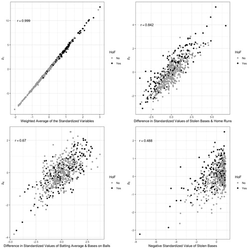
Alternative Application: For the last four retained principal components, the interpretation is not as obvious mainly due to the small magnitudes for the loadings or coefficients and the very weak correlations with the corresponding standardized variables. That makes these interpretations not as obvious. After walking through the thought process on the previous interpretations, ask students to attempt possible interpretations of the last four retained principal components.

3.2 Assessing the Model Fit

For this project (or exercise or example), students created principal components to overcome the issue of multicollinearity in a logistic regression model. A logistic regression model was fit using whether or not the player is in the Hall of Fame as a response variable, where a “success” is that the player is in the Hall of Fame, and the eight principal components as the predictor variables. Table 9 contains the estimated coefficients for the logistic regression model with the eight principal components as the predictor variables. The most significant predictor is the first retained principal component, z₁, given all of the other predictors in the model. Recalling that this principal component represents the weighted average of the standardized original variables, it is not surprising that the coefficient is positive, meaning that as a hitter’s metrics become more large than average, it is more likely that the hitter will be elected to the Hall of Fame, given all other predictors are held constant. The second retained principal component, z₃, is the second most significant predictor, given all of the other predictors in the model. This principal component was interpreted as being a measure of speed versus power based on a difference in the standardized value of SB and the standardized value of home runs. Since this estimated regression coefficient is positive, the larger the difference in these standardized values, the more likely the hitter will be inducted into the Hall of Fame, given that all other predictors are held constant. This difference becomes more positive the more SB a hitter has than average compared to the more home runs a hitter has than average. The principal component z₄ was interpreted to be the difference in the standardized value of batting average and the standardized value of bases on balls. Since this estimated regression coefficient is positive, as a hitter’s batting average becomes better than average compared to a hitter’s bases on balls compared to the average, they are more likely to be inducted into the Hall of Fame, given that all other predictors are held constant. The principal component z₅ was interpreted to be basically the negative of the standardized value of SB. Since this estimated regression coefficient is positive, larger values of z₅ mean the hitter is more likely to be inducted into the Hall of Fame, given that all other predictors are held constant. All things being equal, if a hitter has fewer SB than average, they are more likely to be inducted into the Hall of Fame. This may sound like it is basically the opposite conclusion of the interpretation for the regression coefficient of z₃; however, z₅ is looking solely at SB while z₃ is measuring some combination of speed and power by measuring the difference in SB and home runs, all while holding all other principal components at fixed values.

Table 9 Estimated coefficients for the logistic regression model.

		Estimate	Std. Error	z-value	p-value	VIF
	Intercept	–2.382	0.225	–10.600	$<2\times {10}^{-16}$
z1	Component #1	0.939	0.090	10.483	$<2\times {10}^{-16}$	1.596
z3	Component #3	0.796	0.122	6.529	$6.64\times {10}^{-11}$	1.252
z4	Component #4	0.399	0.170	2.344	0.019	1.131
z5	Component #5	0.588	0.200	2.937	0.003	1.070
z6	Component #6	1.200	0.226	5.314	$1.08\times {10}^{-7}$	1.120
z11	Component #11	–2.274	0.727	–3.129	0.002	1.164
z14	Component #14	–3.317	1.320	–2.513	0.012	1.092
z16	Component #16	–7.000	3.515	–1.992	0.046	1.194

The Hosmer–Lemeshow goodness-of-fit test ($X^2=2.4567$ with 8 degrees of freedom, p-value = 0.9637) indicates that the model is a good fit to the data. This test was performed using the hoslem.test function in the ResourceSelection package (Lele, Keim, and Solymos 2017) in R. See the code in the online appendix for more details. To run this test, the estimated probability of success is calculated for all players in the dataset. These estimated probabilities are ordered into a specified number of groups, in this case 10 groups. In each group, the number of players in the Hall of Fame and not in the Hall of Fame is recorded. These observed counts are compared to the expected counts and a chi-square test statistic is computed. The test statistic is compared to a chi-square distribution with degrees of freedom equal to the number of groups minus two, in this case $10-2=8$.

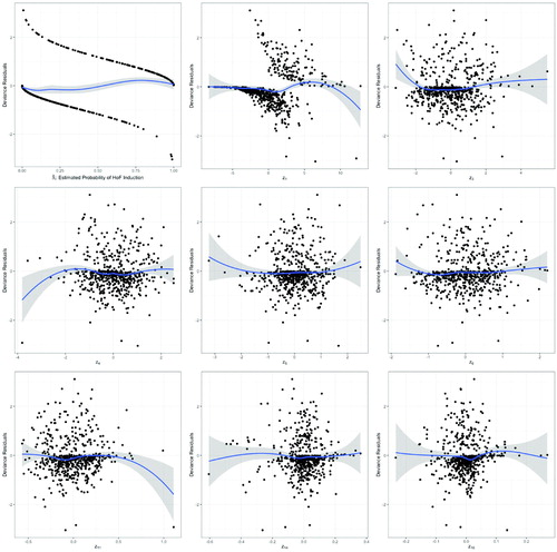
Once the model is fit, residual plots based on the deviance residuals can be plotted versus the model’s fitted values as well as each of the predictor variables. Figure 2 shows the deviance residual plots from the logistic regression model using the eight retained principal components as predictor variables. A loess line is also displayed on each of these plots. If the loess line is as flat as possible, that indicates that the predictor variable should not be transformed when entered into the model. If this curve appears to be quadratic, the predictor variable in question should be transformed as the square of that variable. For the most part, the loess line in all of these plots are fairly flat. This indicates that no further transformation of the predictor variables is needed in this analysis.

Fig. 2 Deviance residual plots versus fitted values and retained principal components.

Table 10 shows the predicted classification of each player based on the results from the logistic regression model. Overall, the model correctly classifies 89.7% of the players (540 out of 602 players). Out of the 447 players not in the Hall of Fame, the model correctly identified 95.1% of them (425 out of 447). For the 155 players in the Hall of Fame, the model correctly identified 74.2% of them (115 out of 155).

Table 10 Player classification: logistic regression model results.

	Model prediction
Actual	No HoF	HoF
No HoF	425	22
HoF	40	115

Helpful Hint: Encourage students to investigate the actual cases that are false negatives (actual Hall of Fame players identified as not worthy of selection) and false positives (players not elected to the Hall of Fame that model thinks should be in the Hall of Fame). The following discussion about Tables 8 and 9 will help the students see where the models went “wrong.”

Table 11 shows the “false positives” in the model, that is, the players predicted to be enshrined into the Hall of Fame but who are not actually members of the Hall of Fame. Of the twenty-three players on the list, five of them (Barry Bonds, Larry Walker, Scott Rolen, Edgar Martinez, Manny Ramirez) are all still eligible to be elected by the BBWAA; however, two of the five players mentioned (Bonds and Ramirez) might not ever be elected to the Hall of Fame due to their ties, either confirmed or alleged, to performance enhancing drugs (Fainaru-Wada and Williams 2006; Tayler 2014). Pete Rose, baseball’s all-time leader in hits, and Shoeless Joe Jackson are two players that are permanently banned from the Hall of Fame for having gambled on baseball games. Bill Dahlen was considered by many to be one of the greatest shortstops in baseball during his playing career from 1891 to 1911; however, “Bad Bill” supposedly fought with teammates, managers, and umpires and anecdotally had a bit of a drinking problem (Womack 2015). These “character issues” may have long turned off voters from voting for him. Many believe that voters have used a similar rationale of character issues for not inducting Dick Allen into the Hall of Fame, even though sabermetricians like Bill James once called Allen “the most gifted baseball player I have ever seen” (James 1987). The player in this table that might be the most curious to see for baseball fans is Nomar Garciaparra. He won the American League Rookie of the Year Award in 1997, came in second in voting for the American League Most Valuable Player Award in 1998, and was selected six times to Major League Baseball’s All Star Game; however, his career was cut short due to injuries.

Table 11 Player classification: predicted Hall of Famers not in the Hall of Fame.

Name	$\widehat{P}\left(\text{HoF}\right)$	Name	$\widehat{P}\left(\text{HoF}\right)$
Pete Rose	0.990	Edgar Martinez	0.671
Barry Bonds	0.986	Vada Pinson	0.660
Shoeless Joe Jackson	0.982	Buddy Bell	0.660
Bill Dahlen	0.888	Ken Boyer	0.624
Lave Cross	0.800	Sherry Magee	0.611
Nomar Garciaparra	0.765	Minnie Minoso	0.590
Kenny Lofton	0.740	Keith Hernandez	0.582
Larry Walker	0.709	Manny Ramirez	0.571
Bobby Veach	0.688	Dick Allen	0.531
Scott Rolen	0.688	Thurman Munson	0.515
Ted Simmons	0.678	Ken Williams	0.508

Table 12 shows the “false negatives” predicted by the model, that is, the players predicted not to be in the Hall of Fame but who are actually members of the Hall of Fame. Twenty-nine out of the forty players (72.5%) were elected by the veterans committees or one of the eras committees. Most of these players elected by these committees, denoted with a dagger in Table 12, played in the pre-integration era of Major League Baseball (prior to 1947, Jackie Robinson’s debut in Major League Baseball). Some of these players played in what is known as the “dead ball” era of baseball, roughly the years 1900 to 1919, prior to Babe Ruth’s emergence as a hitter rather than a pitcher. The game of baseball during this era was more strategy based. Managers would rely on SB and hit-and-run plays—which are plays in which the base runner starts running as the pitcher throws to home plate creating an opportunity to take more bases with a base hit, than on simply using home runs to score (Okrent, Lewine, and Nemec 2000). Players on this list from the dead ball era may have had statistics greater than their peers; however, their statistics pale in comparison to even above average players in its current iteration.

Table 12 Player classification: Hall of Famers predicted not to be in the Hall of Fame.

Name	Years	$\widehat{P}\left(\text{HoF}\right)$	Name	Years	$\widehat{P}\left(\text{HoF}\right)$
Red Schoendienst^†	1945–1963	0.490	Jim Thome*	1991–2012	0.226
Gabby Hartnett*	1922–1941	0.467	Ross Youngs^†	1917–1926	0.225
Dave Winfield*	1973–1988	0.463	Ralph Kiner*	1946–1955	0.225
	1990–1995
Bobby Doerr ^†	1937–1944,	0.419	Lloyd Waner^†	1927–1942,	0.203
	1946–1951			1944–1945
Dave Bancroft ^†	1915–1930	0.417	Freddie Lindstrom^†	1924–1936	0.202
Jim Bottomley^†	1922–1937	0.410	Larry Doby^†	1947–1959	0.200
Tony Perez*	1964–1986	0.395	George Kell^†	1943–1957	0.194
Enos Slaughter^†	1938–1942,	0.395	Ernie Lombardi^†	1931–1947	0.182
	1946–1959
Max Carey^†	1910–1929	0.381	Willie McCovey*	1959–1980	0.174
Lou Brock*	1961–1979	0.368	Joe Tinker^†	1902–1916	0.132
Travis Jackson^†	1922–1936	0.349	Roy Campanella*	1948–1957	0.109
Reggie Jackson*	1967–1987	0.335	Roger Bresnahan^†	1897, 1900–1915	0.107
Harry Hooper^†	1909–1925	0.305	High Pockets Kelly^†	1915–1917,	0.103
				1919–1930, 1932
Joe Gordon^†	1938–1943,	0.302	Phil Rizzuto^†	1941–1942,	0.096
	1946–1950			1946–1956
Tony Lazzeri^†	1926–1939	0.295	Johnny Evers^†	1902–1917,	0.092
				1922, 1929
Hack Wilson^†	1923–1934	0.290	Harmon Killebrew*	1954–1975	0.069
Orlando Cepeda^†	1958–1974	0.275	Bill Mazeroski^†	1956–1972	0.042
Frank Chance^†	1898–1914	0.259	Rick Ferrell^†	1929–1945, 1947	0.028
Willie Stargell*	1962–1982	0.257	Tommy McCarthy^†	1884–1896	0.025
Chick Hafey^†	1924–1935, 1937	0.239	Ray Schalk^† 1912–1929	0.008

† Elected by one of the veterans or eras committees.

* Elected by the BBWAA.

4 Conclusion

The previously discussed analysis is an example on how to use principal components beyond simply reducing the dimensions of a dataset. While one would hope that the logistic regression model’s ability to correctly classify players would be better than what is presented here, it gives students another example of the “joys” of working with real data. After all, the cleanest examples appear in textbooks’ examples for a reason.

The plan is to keep adding to this dataset with every annual vote for hitters’ induction into the Hall of Fame, rerunning the model, and predict which hitters would and would not be in the Hall of Fame. Perhaps with a newer generation of more statistical savvy baseball writers and Hall of Fame voters, the number of “false positives” will decrease and the number of “false negatives” will not increase, making it pretty obvious which hitters are worthy of induction. As far as the “false negatives” go, there is nothing that can be done to really reduce those numbers. Once a hitter is inducted, they cannot be retroactively removed from the Hall of Fame.

Students may wish to further explore principal components analysis, logistic regression, and baseball’s Hall of Fame. This analysis only focuses on hitters. A natural follow-up analysis or project could entail running a similar type of analysis on every pitcher that has received a vote for induction into the Hall of Fame. If baseball is not a sport of interest, and the student wanted to still apply this type of analysis in the field of sports, they could also perform this type of analysis on the National Football League, the National Basketball Association, or the National Hockey League, just to name a few professional sports leagues in North America.

Instructors wishing to use this dataset in their classrooms are not just limited to using principal components analysis or logistic regression. These data can be used in introductory statistics classes when discussing the robustness of the two-sample t-test or performing a randomization test on a variable of one’s choice to compare the difference between Hall of Fame and non-Hall of Fame players. Even though not all students follow baseball, with enough guidance, students should figure out that the Hall of Fame players should typically have greater values for the various variables than the non-Hall of Fame players.

Supplementary Materials

The R code was used to read the file baseballHOF.csv into R, fit the multiple regression model, calculate the variance inflation factors, and to generate the correlation matrix. All figures were generated using the ggplot2 package (Wickham 2016) in R.