A Web Simulator to Assist in the Teaching of Bayes’ Theorem

Abstract

Teaching some concepts in statistics greatly benefits from individual practice with immediate feedback. In order to provide such practice to a large number of students we have written a simulator based on an historical event: the loss in May 22, 1968, and subsequent search for the nuclear submarine USS Scorpion. Students work on a simplified version of the search and can see probabilities change in response to new evidence. The simulator is designed to assist in the teaching of Bayesian concepts, in particular Bayesian updating. It has been deployed in our courses and our experience and results are described, as well as the reactions of our students to its use. The simulator is open source, freely available and easy to implement and run, as it only requires a machine to serve web pages. We explain in detail our experience with its deployment and use.

Keywords:

• Bayesian statistics
• Statistics
• Simulator

1 Introduction

Bayes’ theorem, in its simplest form expressible as (1) $$P\left(A\right|B)=\frac{P\left(B\right|A\left)P\right(A)}{P\left(B\right)},$$(1) provides a way to “invert” probabilities: from the conditional probability of B given A and the respective marginals, the probability of A given B can be computed. Although it is simple and can be presented and proved in a matter of minutes, this is a concept that requires time for students to grasp.

We have found useful over the years to present some examples that help enhance student’s comprehension of the practical implications of (1). Medical diagnosis is one: the probability $P(A|B)$ of having a sickness A given the presence of symptom B can be obtained in terms of the probability of the symptom given the sickness and the respective marginal probabilities of sickness and symptom. This nicely illustrates the way to revise a prior P(A) in the light of newly available information B.

Acquiring familiarity with the concepts involved requires, much as the acquisition of a new language, repeated interaction with (1), beyond the few examples that can be presented in class. Such familiarity can be fostered by assigning homework to be done by students and later graded, but this imposes a considerable burden on the teachers and provides, at best, delayed feedback to the student. We thought that a simple simulator, presenting each student a unique instance of a problem, with immediate feedback and automatic grading, would be much preferable. This article reports on our work in this direction.

Section 2 reviews some work which addresses similar goals as ours or which we have otherwise used for inspiration. Section 3 briefly describes the story we have used, in a simplified recreation, to motivate a game in which students are required to locate a missing submarine. Section 4 describes the implementation. We tested the use of our simulator on our introductory course on statistics to sophomores, when Bayes’ theorem is first presented; Section 5 gives some details about the results obtained. Section 6 closes with some comments.

2 Motivation and Available Resources

2.1 Motivation

In the last few decades, there has been a clear trend toward Bayesian statistics which was previously almost entirely neglected by practicing statisticians: McGrayne (2012) tells the fascinating history. However, this trend seems to have been much slower in statistical teaching in spite of vigorous allegations advocating for change (Cobb 2015; Witmer 2017).

In our courses, Bayes’ theorem is introduced at a very early stage, just three weeks after starting the first introductory course to Statistics and Data Analysis. We consider this early introduction of the utmost importance, even if statistical techniques taught later are (still) classical in the main. It gives students a broader perspective which helps them understand the frequentist interpretation of probability first, then of inference (Page and Satake 2017, p. 263, further elaborates this point).

On the other hand, at least for some students, it is thrilling to find right at the very beginning of the subject a still controversial question about what it is the “right” way to learn from data.

2.2 Available Resources

In an attempt to introduce some practice in Bayesian statistics beyond simple classroom examples, we searched the Internet for teaching aids. We did not find anything covering, in a simple way, the precise topic we wanted our students to practice (Bayesian updating of probabilities), although there are abundant resources which make use of games or simulations of some sort. Most examples we have found are related to experimental design and some have a history that goes back to pioneering papers Mead and Stern (1973) and Pike (1974); see Stern, Latham, and Stern (2009) for instance.

Closer to our goal of introducing students to the rudiments of Bayesian thinking is Erickson (2017), which proposes two examples of activities. It emphasizes graphical aids in the form of mosaic plots to help build intuition. Downey (2012) is a wonderful book with lots of worked examples that guide the reader who is reasonably proficient in Python. It could be adapted to use with R, which is prevalent at our institution, but still would require more skills in programming than we can assume of most of our students. Witmer (2017), in turn, presents an experience of introducing Bayesian ideas through Markov chain Monte Carlo (MCMC) at the undergraduate level.

Our goal is less ambitious: we wanted a simple teaching aid to help understand the very foundations of Bayesian thinking, namely how a priori probabilities are updated to a posteriori probabilities in the light evidence, and how these a posteriori become established a priori knowledge to be used at a next step. We did not find a tool to do exactly that, which led us to develop the simulator described in Section 4 around the story in Section 3 next.

3 The Loss of the USS SCORPION

3.1 The History

The USS Scorpion was a nuclear submarine in the U.S. Navy. It disappeared on May 22, 1968, close to the Azores archipelago, when returning to its base in Norfolk from a mission. The reasons are as yet uncertain. There was speculation about an explosion, accidental activation of a foul torpedo, a Soviet attack, and various malfunctions.

After several days elapsed without contact, the search for the submarine started. The vicinity of the last known position of the ship was divided in 400 sectors. An a priori probability of containing the remaining of the ship, using available information and expert’s assessments, was ascribed to each such sector.

The search was conducted using methods of Bayesian search theory, on the advice of statistical experts. These methods had been used with success in the search of a hydrogen bomb accidentally dropped by a B52 bomber off the southern coast of Spain, near Palomares, in 1966. The search for the USS Scorpion also ended with success in October 1968, when parts of the submarine were found in the sea bed under 3000 m of water, some 400 nautical miles southwest of the Azores.

Both Cressie and Wikle (2011) and McGrayne (2012) contain statistically oriented accounts of the USS Scorpion search. Wikipedia also has a good account and a number of pointers to other sources of information. An interesting follow-up, more technical, is Davey et al. (2016), presenting Bayesian search techniques in the case of the lost Malaysian Air Lines flight MH370, in 2014. We closely follow the first reference in the short summary of relevant theory next.

3.2 Bayesian Approximation

Let Y_i be a random variable with two states: Y _i = 0 means “The submarine is not present in sector i,” while Y _i = 1 means the opposite.

Likewise, let X_i be a random variable coding the outcome of searching a sector i. Let X_i = 0 if the submarine is not found in said sector and X_i = 1 if it is.

Clearly X_i is dependent on Y_i :

• If the submarine is not present in the ith sector, it cannot possibly be located in that sector, so: $$P(X_i=1|Y_i=0)=0.$$

• On the other hand, if it is indeed present in the ith sector, the probability that it will be found is p: $$P(X_i=1|Y_i=1)=p.$$

A search is not guaranteed to be successful, so p < 1: there is a nonzero probability that we fail to detect the submarine in a search of the ith sector, even though it is really there.

Assume that the a priori probability of the submarine being in the ith sector is π_i. If we search that sector to no avail, the probability a posteriori that the ship is there is, using (1) (2) $$\begin{array}{c}P(Y_i=1|X_i=0)=\frac{P(X_i=0|Y_i=1\left)P\right(Y_i=1)}{P(X_i=0)}\\ =\frac{P(X_i=0|Y_i=1\left)P\right(Y_i=1)}{\begin{array}{c}P(X_i=0|Y_i=0\left)P\right(Y_i=0)\hfill \\ \hspace{1em}+P(X_i=0|Y_i=1\left)P\right(Y_i=1)\hfill \end{array}}\\ =\frac{(1-p){\pi }_i}{1\times (1-{\pi }_i)+(1-p){\pi }_i}\\ ={\pi }_i\frac{(1-p)}{1-p{\pi }_i}\end{array}$$(2)

We call the attention of students on the fact that, as intuition suggests, failure to locate the submarine in a search of sector i does not preclude the possibility that it is there, but makes the posterior probability smaller than the prior probability: the ratio $$\frac{(1-p)}{1-p{\pi }_i}$$ which multiplies π_i in 2 is less than one, the more so the greater p is.

As a consequence of a fruitless search of sector i, the probabilities of all others sectors are also modified. For $j\cancel{=}i$, we have (3) $$\begin{array}{c}P(Y_j=1|X_i=0)=\frac{P(X_i=0|Y_j=1\left)P\right(Y_j=1)}{P(X_i=0)}\\ =\frac{1\times {\pi }_j}{1-p{\pi }_i}\\ ={\pi }_j\frac{1}{1-p{\pi }_i}.\end{array}$$(3)

Again as intuition suggests, the fact that the submarine is not located by a search of sector i enhances our belief that it is in any of the sectors $j\cancel{=}i$, for the factor that multiplies the prior probability π_j in (3) is greater than one.

4 The Simulator: Use and Implementation

4.1 Design Goals

We did not seek a tool to introduce Bayes’ theorem, but rather a tool to practice theory previously learned although perhaps not fully internalized. Consequently, Bayes’ theorem and its application to the problem at hand is taught in class, roughly along the lines of Section 3.2, and a handout describing the practice and how to use the simulator is given in advance to students.

We had to serve a large number of students, not all of them in one location. This, in practice, reduced the choices to a web-based simulator, requiring nothing else on the client side other than a Javascript-enabled web browser. Students can use the simulator from any computer room on campus or from their own computers at home. The implementation is light, runs off a single server and can be easily understood and changed. Simulation parameters like the number of initial regions, parameter p, generation of initial a priori probabilities, etc. require fairly simple changes to the source.

4.2 Setup

Our simulator faces the student with the same decisions that the search team of the USS Scorpion had to make, but in a rather simplified setting: instead of 400 sectors only nine are presented in a map (see Figure 1). Prior to use of the simulator, students are given a write-up containing essentially the information given in Section 3 of the present article.

Fig. 1 Initial screen of simulator.

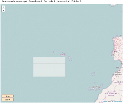
To start using the simulator, the student only has to press the button Start in the bottom left corner. The simulator then generates a random instance of the game assigning a priori probabilities to all nine searchable sectors and places a search vessel next to the southwest corner of the searchable area. Clicking on any one sector gives information on its a priori probability at any time; this probability is also encoded as color saturation in a palette of greens¹ (Figure 2).

Fig. 2 Simulator screen after one correct but unsuccessful search.

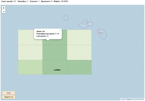
The first search is trivial: just go to the sector with higher a priori probability. In order to do that, the student just has to drag with the mouse the search vessel to the sector chosen and either click on it or on the button Search in the southwest corner; the latter alternative has been found necessary for players using small screens such as tablets or cellular phones.

After each student’s choice, the simulator updates the counters at the top of the page (last sector searched, number of searches, “correct” and incorrect searches, points earned). A search is “correct” if the sector with the largest probability is chosen. Points earned are ten times the ratio of correct to total searches, so a score of 10 means that the student chose every time to search the most likely rectangle.

The simulator will tell the student whether the submarine is found, in which case the game ends, or else update the a priori probabilities of each of the sectors, in light of the last fruitless search. These updated probabilities, though, are neither displayed nor color-encoded in the screen, which always shows probabilities prior to the last search: the π_i of Equations 2(2) $$\begin{array}{c}P(Y_i=1|X_i=0)=\frac{P(X_i=0|Y_i=1\left)P\right(Y_i=1)}{P(X_i=0)}\\ =\frac{P(X_i=0|Y_i=1\left)P\right(Y_i=1)}{\begin{array}{c}P(X_i=0|Y_i=0\left)P\right(Y_i=0)\hfill \\ \hspace{1em}+P(X_i=0|Y_i=1\left)P\right(Y_i=1)\hfill \end{array}}\\ =\frac{(1-p){\pi }_i}{1\times (1-{\pi }_i)+(1-p){\pi }_i}\\ ={\pi }_i\frac{(1-p)}{1-p{\pi }_i}\end{array}$$(2) and (3). It is the student’s task to do the updating using these formulas.

Students are told the value of p—the probability that a search of the right rectangle will unveil the submarine—which in the experiment described later was set at p = 0.60. They can be told or allowed to discover by themselves that, as they proceed with the game, they only have to update two probabilities: that of the recently searched sector, which might remain the most promising in spite of a failed attempt, and that of the previously most likely sector—since the Bayesian updating multiplies the a priori probability of all sectors different from the one just searched by the same factor and so preserves their order; see Equation (3)(3) $$\begin{array}{c}P(Y_j=1|X_i=0)=\frac{P(X_i=0|Y_j=1\left)P\right(Y_j=1)}{P(X_i=0)}\\ =\frac{1\times {\pi }_j}{1-p{\pi }_i}\\ ={\pi }_j\frac{1}{1-p{\pi }_i}.\end{array}$$(3) .

The game ends when the submarine is finally located, and the points earned are saved. It is up to the instructors to let the students play once or (our choice) as often as they wish, keeping only their last score.

4.3 Implementation Aspects

The simulator is coded in Javascript using the library leaflet² for the map presentation.

We cheated a bit in the implementation. In fact, the submarine is not randomly allocated to any sector. What we randomize at the start of the game is the minimum number of trials the student will have to go through: this is to avoid events like finding the submarine at the first trial, that would give the maximum score without a record of consistently good search choices. No matter what, the student will have to make a number of searches (at least six in the current implementation, but this is easy to change), so we can be assured that a score of 10 means consistent good use of Bayes updating and not just a lucky single choice that finds the submarine on the first or second random attempt.

Another aspect that teachers might want to fine tune is the parameter p—the probability of success when searching the correct sector. It follows from the previous paragraph that it has no influence in the length of the game, but it does have a large influence in the updating of the a priori probabilities. If set too high, an unsuccessful search will dramatically lower the posterior probability of the searched sector: the subsequent choice will then almost invariably be the sector that had the largest a priori probability before the last search. Students might soon notice the pattern and play with no resort at all to formulas in Equations (2)(2) $$\begin{array}{c}P(Y_i=1|X_i=0)=\frac{P(X_i=0|Y_i=1\left)P\right(Y_i=1)}{P(X_i=0)}\\ =\frac{P(X_i=0|Y_i=1\left)P\right(Y_i=1)}{\begin{array}{c}P(X_i=0|Y_i=0\left)P\right(Y_i=0)\hfill \\ \hspace{1em}+P(X_i=0|Y_i=1\left)P\right(Y_i=1)\hfill \end{array}}\\ =\frac{(1-p){\pi }_i}{1\times (1-{\pi }_i)+(1-p){\pi }_i}\\ ={\pi }_i\frac{(1-p)}{1-p{\pi }_i}\end{array}$$(2) and (3)(3) $$\begin{array}{c}P(Y_j=1|X_i=0)=\frac{P(X_i=0|Y_j=1\left)P\right(Y_j=1)}{P(X_i=0)}\\ =\frac{1\times {\pi }_j}{1-p{\pi }_i}\\ ={\pi }_j\frac{1}{1-p{\pi }_i}.\end{array}$$(3) —which defeats the purpose of the simulator. It is therefore advisable to set p at a moderate value. We have tried in the vicinity of 0.6 with good results.

5 Deployment and Results

We have tested the simulator with undergraduate students taking a first quarter in statistics, covering probability, random variables, density and distribution functions, moments, characteristic function, etc. which lay the foundation for a second quarter on Inferential Statistics. It is in this course that Bayes’ theorem is first discussed.

Our students are all in the sophomore year of Business, Economics or Business and Law degrees. The last group (double major in Business and Law) tend to be composed of better performing students, as the entrance requirements are stricter. The mathematical background of all groups is similar: two quarters of Calculus and Algebra.

5.1 Test

We devised a short exam with questions in which students were required to recognize whether the use of the word “probability” had a Bayesian or frequentist flavor. For instance,

When we say that the probability that the Malaysian Airlines plane lost in 2014 (flight MH370) is in a given area in the Pacific ocean with probability p = 0.01, are we using the word ‘probability’ in a Bayesian or in a frequentist sense?.

We also included the simplest problem we could think of which required sequential application of Bayes’ theorem—what the simulator is designed to provide training for. It read,

1. In a foggy day, a hiker suffers an accident when returning from a mountain. He believes that with probability 0.60 he is in the North slope, but with probability 0.40 he might have ended in the South slope. Before using his cellular phone to ask for help, he would like to better fix his location. He remembers that in the North slope beech trees are prevalent (70% of the total) with the rest being oak trees (15%) and yew trees (15%), while in the South slope the proportions are 30% beech trees, 60% oak trees and 10% yew trees. He approaches the nearest tree and realizes that it is an oak tree. Using this information, the probability that he is in the North slope is, approximately$\dots$

   This is a simple example in which students can use the available information to revise their prior probability and obtain a posterior probability. This was followed by:

2. After having found the tree mentioned in the previous question, he walks further and finds another tree, which he recognizes as being a yew tree. He then falls to the ground, exhausted. Where will he tell the rescue brigade to search for him, in the North or South slope?

The intent is to go one step further. Here, we want the student to recognize that the posterior from (a) can be used as a prior in (b)—the essence of Bayesian learning that our simulator targets.

5.2 Assessment Method

Our first thought was to devise a standard experiment, either randomizing the “treatment” (= use of simulator) or taking pairs of students matched according to their ability (measured by their grade point average, for instance) and assigning within each pair one to the group of simulator users and the other to the group of nonusers. We would then compare performance of both groups when taking the test described in the previous section.

However, since the test was to give credit toward the course grade this would create an unfairness toward the students that were not assigned to the simulator group. This, in our context, cannot be contemplated. On the other hand, there is no way in which we could ensure that the untreated or control group was really untreated: out of curiosity or otherwise any student could use the simulator and thus contaminate the control group.

We therefore decided that we would administer the test twice, before and after giving a chance to use the simulator. We were fully aware that the second time the test is taken a better performance is to be expected, even for nonusers of the simulator. But we counted on measures of use of the simulator (time spent, score obtained when using it) as well as on having some accidental “controls”: students who for various reasons would not use the simulator. That would enable us to disentangle the effect of using the simulator and the effect of mere repetition of the test. As it happens, the control group was larger than we expected.

After covering Bayes’ theorem in class, we required students to take the test described above. They were then encouraged to freely use the simulator for a period of five days: this free use policy and the fact that only the last score would be recorded was made clear to them beforehand, as well as the fact that use of the simulator might be of some help in a second test.

Then, the same test was given again, complemented with a few questions regarding whether they had found the use of the simulator to be easy, rewarding, how much time they had spent on it, etc.

The fact that we have the same students take the first and second tests enables us to account for differences in student ability. The problem, of course, is that there can be a self-selection effect: more motivated students might choose to use the simulator in greater proportion than the others. Below we report on some evidence of this effect in the results: it may have been countered by the fact that better performing students, after obtaining a good grade in the first test, did not see room for improvement and therefore neglected the use of the simulator.

5.3 Results and Modeling

Both tests were administered in the Fall Term of 2017 in the form of multiple choice questionnaires, to avoid any subjective biases from the graders. As Figures 3 and 4 imply, they were graded on a 0–10 scale (the color-coded simulator scores were also in a 0-10 scale).

Fig. 3 Breakdown on grades in pre- and post-test according to use of simulator.

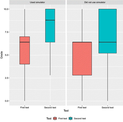
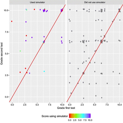
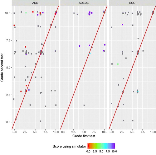
Fig. 4 Individual performances in pre- and post-test according to use of simulator and score obtained. Each point is color-coded reflecting the score obtained when using the simulator (right legend), with students who did not use it shown in gray.

A total of 241 students participated, but 52 were absent in either the first or second test (pre- and post-test in the sequel). Therefore, we observed 189 students who took both the first and second test plus 52 who only took one of the tests.

Figure 3 shows the breakdown of grades of the common set of questions in the pre- and post-test. (Subjective questions in the post-test as to whether the simulator had been useful, fun, etc. were not graded.)

Clearly, there is an improvement, particularly apparent in the larger median grade for the subset of students that used the simulator. Also, grades below 2.5 points were entirely absent among the simulator users.

A different, more insightful view, is provided by Figure 4. The performance of each student is shown by a point, whose coordinates are the grades in the first and second test. (Points have been jittered, to reduce overploting.) The two panels show the performance of students who did and did not use the simulator. Further, for those who did use the simulator, the score obtained is color-coded in the left panel. The red lines mark show equal grades in the first and second tests: points above the red line indicate an improvement.

We expected all scores using the simulator to be equal or close to the maximum 10, given our policy of “use for as long as you wish, keep only your last grade.” As a matter of fact, this has not been the case: some students abandoned the task earlier with low or even zero scores. However, although improvement in the second test is not clearly related to the simulator score, it seems much more consistent among students who used the simulator, whatever score they obtained.

When we break down the results by group, Figure 5, we find that students in the ADEDE group (double degree in Business and Law) did much better than students in either of the single degrees of Business (ADE) or Economics (ECO). It is apparent also that ADEDE students not only obtained higher scores when using the simulator, but also used it in a larger proportion (more colored points in Figure 5), which points to a possible problem of sample self-selection addressed earlier.

Fig. 5 Breakdown of grades in pre- and post-test according to use of simulator per group. Each point is color-coded reflecting the score obtained when using the simulator (right legend), with students who did not use it shown in gray.

To obtain a more formal assessment of the effect of the simulator, we have fitted several linear models. A natural approach would be to consider for each student the difference in grades obtained in the first and second test as a response variable, and relate that difference to the use (or not) of the simulator, and possible other factors. In other words, to use a paired comparisons approach.

However, a total of 52 observations are not paired: some students took the first test and not the second or vice versa. In order to use also these observations, we have fitted several linear mixed models, Demidenko (2004), in which the response variable is the grade obtained in either of the tests. Differences in the individual performance of students are accounted for by a random effect, as individuals are of no interest in themselves. The simulator effect, “repeat” effect, and group effect are introduced as fixed effects. All models have been fitted in R, R Core Team (2017), using package lme4 (see Bates et al. 2015).

Model 1 is, in the usual notation, $$\mathit{Grade}=1+\left(1\right|\mathit{ID})+\mathit{Rep};$$ variable Rep is a dichotomous variable taking value 0 for 230 observations corresponding to the first test and 1 for 200 observations corresponding to the second. (1—ID) is a random term, different for each student and reflecting his or her individual ability. It is of no interest in itself—we know students to be different—but useful to allocate the part of variance that is explained by student’s heterogeneity.

The coefficient of Rep (the “repeat” effect) is positive and highly significant (refer to column Model 1 in Table 1). Its value in this model reflects the (possible) effect of the use of the simulator for some students, as well as the fact that (for all) better performance should be expected the second time the students took the test, irrespective of whether or not they used the simulator.

Table 1 Effect on Grade of use of simulator.

	Model 1	Model 2	Model 3
(Intercept)	5.60${}^{***}$	5.61${}^{***}$	5.25${}^{***}$
	(0.18)	(0.18)	(0.22)
RepYES	1.24${}^{***}$	0.99${}^{***}$	1.04${}^{***}$
	(0.22)	(0.24)	(0.24)
Used.simYES		1.08${}^{*}$	0.75
		(0.44)	(0.45)
GroupADEDE			2.12${}^{***}$
			(0.48)
GroupECO			0.40
			(0.32)
AIC	2083.28	2079.17	2064.15
BIC	2099.53	2099.49	2092.60
Log-likelihood	–1037.64	–1034.58	–1025.08
Num. obs.	430	430	430
Num. groups: ID	241	241	241
Var: ID (Intercept)	2.66	2.52	2.13
Var: Residual	5.04	5.06	5.07

NOTE:

*** $p<0.001,$

** $p<0.01$, and

* $p<0.05$.

To disentangle the effect attributable to the simulator from that of mere repetition of the exam, we can fit the model $$\mathit{Grade}=1+\left(1\right|\mathit{ID})+\mathit{Rep}+\mathit{Used}.\mathit{sim},$$ where Used.sim is a dichotomous variable taking value 1 for observations corresponding to the second test of students who did use the simulator. The estimation results can be seen in column “Model 2” of Table 1. A test of Model 2 versus Model 1, see Table 2, shows a decrease of 5.922 in deviance, highly significant (p = 0.015). (There is a very small mismatch with the values of the log-likelihood and model criteria AIC and BIC reported in Table 1, possibly consequence of different methods of computing the log-likelihood and degrees of freedom.)

Table 2 Comparison of models.

Model	AIC	BIC	logLik	Deviance	Chisq	Pr($>$Chisq)
1	2080.2	2096.4	−1036.1	2072.2
2	2076.2	2096.6	−1033.1	2066.2	5.9221	0.01495${}^{*}$
3	2061.0	2089.4	−1023.5	2047.0	19.2884	6.48e-05${}^{***}$

However, when we fit the model $$\mathit{Grade}=1+\left(1\right|\mathit{ID})+\mathit{Rep}+\mathit{Used}.\mathit{sim}+\mathit{Group}$$

(results in column Model 3 of Table 1), the coefficient of Used.sim becomes non-significant: it seems that it is partly confounded with the Group effect. This was to be expected since, as it is apparent from Figure 5, students in group ADEDE, who are clearly better performers, have also used the simulator in greater proportion. The Group effect is of paramount importance and accounts for a decrease of 19.288 in deviance, reducing the variance accounted by the random effect ID from 2.52 to 2.13, a reduction of about 15%: part of the heterogeneity among students is in fact a difference between groups.

5.4 Student’s Feedback

The second test included a few questions regarding the experience with the simulator. Students were told that these questions had no reflect whatsoever in their grades, but response was nonetheless total among students having used the simulator.

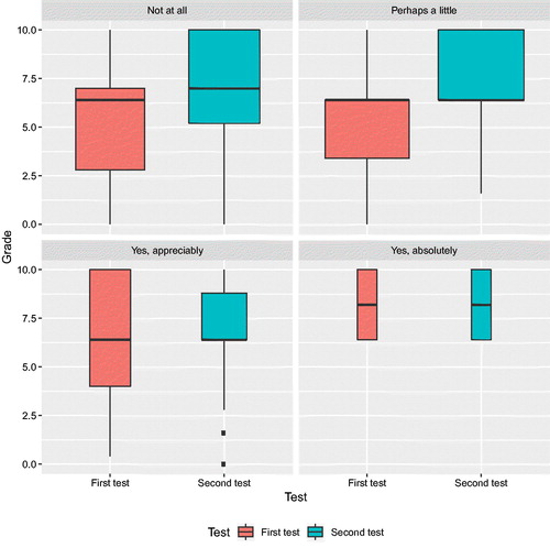
Their perception of whether playing with the simulator was of any help did not clearly correlate with their performance—see Figure 6. Whether they said it had been of no, little, moderate or significant help, their performance in the second test appears to be better—except perhaps, quite paradoxically, for those who were more convinced of the usefulness of the simulator. This may be due to the fact that they were good performers in the first test and therefore with little room for improvement.

Fig. 6 Breakdown of grades in pre- and post-test according to perceived usefulness of the simulator. Students responded that it helped$\dots$

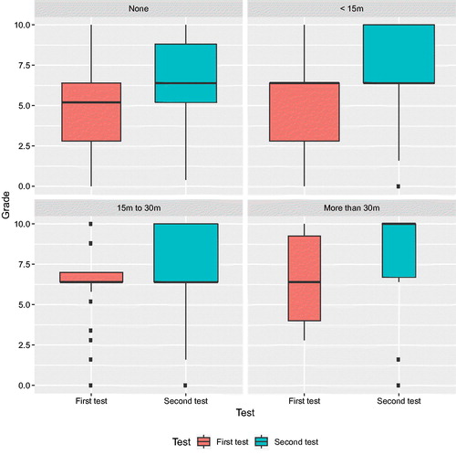
On the other hand, when asked about how much time they spent playing with the simulator, there seems to be a clear pattern of greater improvement for those who spent more than 30 minutes on the simulator: see Figure 7. The median grade went from 6.4 to the maximum of 10; for all the other categories, an upward shift in grades is visible, but—except for the “None” category—the medians remain the same. It is also apparent that those that used the simulator had a higher median grade in the first test.

Fig. 7 Breakdown of grades in pre- and post-test according to time spent using the simulator.

6 Discussion

The evidence we can present on the impact of the simulator is not conclusive: the partial confounding with group effect prevents us from making strong claims about the usefulness of the simulator. However, what we can learn from the observational data in conjunction with the opinions of the students make us believe that it has been of some use.

We plan to extend our work building simulators targeting this sort of topic, which can best be learned by practice and example. Interestingly, some of the examples that lend themselves to implementation in a format similar to the simulator presented here were anticipated in Mead and Stern (1973) and Pike (1974). It is a reflection of the tremendous leap forward in the use of computer-based instruction that what was almost visionary then can be implemented with reasonable effort and very limited resources in our days.

6.1 Accessibility and Teacher Guidelines

The simulator is accessible at http://www.et.bs.ehu.es/bayes and source is available at https://github.com/FernandoTusell/BayesSim.git. We welcome use by third parties, corrections and additions, best of all in the form of pull requests.

The user interface is available in both English and Spanish, in separate branches of the repository referenced above. Even teachers with no experience in web programming will find it easy to customize the source, changing parameters such as the p referred to in Section 4 or labels in the user interface (e.g., “Student ID” rather that “ID card”); or changing them to their language of choice.

No installation is necessary, just a single Javascript source file needs to be dropped in a directory that is served in the web. In the simple setup we have used, student’s grades are written each in a single file, named with the ID number of the student; thus, each subsequent use of the simulator obliterates the previous grade: this is easy to change, just pasting a timestamp to the student number when naming the file. When the period of use of the simulator is over, it is a simple matter to grab all these files to generate a listing.

Of course, a more elegant approach is to store the grades using a database manager, but this will require coding the interface which in turn is dependent of the database software available. We have found our simple approach to work well and be easiest to replicate.

A document of guidelines is available at the repository along with the sources.

Ethics Committee Approval. This research has been cleared with the IRB of our University.

Acknowledgments

We acknowledge partial support of our project from the Servicio de Asesoramiento Educativo (SAE) and GIU17/011 of the University of the Basque Country, UPV/EHU. We also thank the authors of R packages not elsewhere acknowledged in text: ggplot2, Wickham (2009), and texreg, Leifeld (2013), whose availability have eased our preparation of this article. The article has benefited from the constructive criticism of three referees and the editors of the journal, which we also acknowledge.

Notes

Notes

1 A different palette, less visually pleasing, is available for color blind students, should the need arise.

2 See http://leafletjs.com.

References

- Bates, D., Mächler, M., Bolker, B., and Walker, S. (2015). “Fitting Linear Mixed-Effects Models Using lme4,” Journal of Statistical Software, 67, 1–48. DOI: 10.18637/jss.v067.i01.
- Cobb, G. (2015). “Mere Renovation is Too Little Too Late: We Need to Rethink our Undergraduate Curriculum from the Ground Up,” American Statistician, 69, 266–282. DOI: 10.1080/00031305.2015.1093029.
- Cressie, N., and Wikle, C.K. (2011), Statistics for Spatio-Temporal Data, Hoboken, NJ: Wiley.
- Davey, S., Gordon, N., Holland, I., Rutten, M., and Williams, J. (2016), Bayesian Methods in the Search for MH370, Australia: Springer Open.
- Demidenko, E. (2004), Mixed Models: Theory and Applications, Hoboken, NJ: Wiley-Interscience. ISBN: 9780471601616.
- Downey, A. (2012), Think Bayes. Bayesian Statistics Made Simple, Needham, MA: Green Tea Press.
- Erickson, T., (2017), “Beginning Bayes,” Teaching Statistics, 39, 30–35. DOI: 10.1111/test.12121.
- Leifeld, P. (2013), “texreg: Conversion of Statistical Model Output in R to LATEX and HTML Tables,” Journal of Statistical Software, 55, 1–24, available at http://www.jstatsoft.org/v55/i08/.
- McGrayne, S. (2012), The Theory That Would Not Die: How Bayes’ Rule Cracked the Enigma Code, Hunted Down Russian Submarines, and Emerged Triumphant from Two Centuries of Controversy, New Haven: Yale Univ. Press.
- Mead, R., and Stern, R. (1973), “The Use of the Computer in the Teaching of Statistics” (with discussion), Journal of the Royal Statistical Society, Series A, A136, 191–225. DOI: 10.2307/2345109.
- Page, R., and Satake, E., (2017), “Beyond P Values and Hypothesis Testing: Using the Minimum Bayes Factor to Teach Statistical Inference in Undergraduate Introductory Statistics Courses,” Journal of Education and Learning, 6, 254–266. DOI: 10.5539/jel.v6n4p254.
- Pike, D. (1974), “Statistical Games as Teaching Aids,” Journal of the Royal Statistical Society, Series D, D25, 109–115. DOI: 10.2307/2987643.
- R Core Team (2017), R: A Language and Environment for Statistical Computing, Vienna, Austria: R Foundation for Statistical Computing, available at https://www.R-project.org/.
- Stern, D., Latham, S., and Stern, R. (2009), “Statistical Games to Support Problem-based Learning,” IBS SUSAN Conference Proceedings, available at http://www.reading.ac.uk/ssc/resources/Docs/SUSAN/Statistical_Games_to_supportproblem-based_learning.pdf.
- Wickham, H. (2009). ggplot2: Elegant Graphics for Data Analysis, New York: Springer-Verlag.
- Witmer, J. (2017). “Bayes and MCMC for Undergraduates,” American Statistician, 71, 259–264. DOI: 10.1080/00031305.2017.1305289.